Urban Structure and Mobility as Spatio-temporal complex Networks

(1)

Urban Structure and Mobility as Spatio-temporal

complex Networks

Doctoral Thesis

by

Gevorg Yeghikyan

Doctoral Program in Data Science

Supervisor

Mirco Nanni, ISTI-CNR, Pisa

Supervisor

Angelo Facchini, IMT, Lucca

Supervisor

Marco Conti, ISTI-CNR, Pisa

Supervisor

Andrea Passarella, ISTI-CNR, Pisa

Supervisor

Bruno Lepri, FBK, Trento

© Gevorg Yeghikyan, 2020. All rights reserved.

The author hereby grants to Scuola Normale Superiore di Pisa permission to reproduce and to distribute publicly paper and electronic copies of this thesis document in whole or in part in any medium now known or hereafter created.

(2)

Urban Structure and Mobility as Spatio-temporal complex

Networks

by

Gevorg Yeghikyan

Tuesday 16th _{June, 2020 01:42}

Submitted to the Scuola Normale Superiore di Pisa in June 2020, in partial fulfillment of the requirements for the

Doctoral Program in Data Science

Abstract

Contemporary urban life and functioning have become increasingly dependent on mobility. Having become an inherent constituent of urban dynamics, the role of urban moblity in influencing urban processes and morphology has increased dramat-ically. However, the relationship between urban mobility and spatial socio-economic structure has still not been thoroughly understood. This work will attempt to take a complex network theoretical approach to studying this intricate relationship through • the spatio-temporal evolution of ad-hoc developed network centralities based

on the Google PageRank,

• multilayer network regression with statistical random graphs respecting net-work structures for explaining urban mobility flows from urban socio-economic attributes,

• and Graph Neural Networks for predicting mobility flows to or from a specific location in the city.

Making both practical and theoretical contributions to urban science by offering methods for describing, monitoring, explaining, and predicting urban dynamics, this work will thus be aimed at providing a network theoretical framework for developing tools to facilitate better decision-making in urban planning and policy making.

Keywords: urban mobility, machine learning, complex networks, socio-economic attributes, spatio-temporal activity, neural networks

(3)

Publications

As main author

1. Gevorg Yeghikyan, Felix L Opolka, Mirco Nanni, Bruno Lepri, and Pietro Lio. Learning mobility flows from urban features with spatial interaction models and neural networks. arXiv preprint arXiv:2004.11924, 2020 (to appear in the Proceedings of IEEE International Conference on Smart Computing (SMART-COMP 2020))

2. Gevorg Yeghikyan, Leandro Tortosa, Jose F Vicent, and Mirco Nanni. Rank-ing places in attributed temporal urban mobility networks. PloS one, 2020 (under review)

As co-author

1. Manuel Curado, Leandro Tortosa, Jose F Vicent, and Gevorg Yeghikyan. Anal-ysis and comparison of centrality measures applied to urban networks with data. Journal of Computational Science, page 101127, 2020

2. Manuel Curado, Leandro Tortosa, Jose F Vicent, and Gevorg Yeghikyan. Un-derstanding mobility in Rome by means of a multiplex network with data. Journal of Computational Science, 2020 (under review)

3. Leandro Tortosa, Jose F Vicent, and Gevorg Yeghikyan. A centrality measure based on the Adapted PageRank Algorithm for multiplex networks with data. Applied Mathematics and Computation, 2020 (under review)

Conferences

1. IEEE International Conference on Smart Computing (SMARTCOMP 2020), Bologna, Italy

2. Italian Regional Conference on Complex Systems, (CCS Italy 2019), Trento, Italy

(4)

(5)

Acknowledgments

This work would not have been possible without the support, advice, and encour-agement on the part of my supervisors Mirco Nanni, Angelo Facchini, Bruno Lepri, Andrea Passarella, and Marco Conti, to whom I owe very much.

I would also like to thank Dino Pedreschi - the coordinator of the joint Data Science PhD program I had the honor of being part of - for making the research infrastructure and collaborations within the PhD ecosystem possible.

Special thanks also go to other members of the Data Science PhD board as well as individuals connected to the program who have rendered support to my research activities: Anna Monreale, Fosca Giannotti, Tiziano Squartini, Diego Gar-laschelli, Tommaso Cucinotta, Francesca Chiaromonte, Luca Pappalardo, Salvatore Rinzivillo, Ioanna Miliou, Vittorio Romano, and Silvia Zappulla.

The pleasure and ease of working with my co-authors from institutions outside of the Data Science PhD ecosystem - Felix Opolka, Pietro Lio’ from Cambridge University, Vahan Nanumyan from ETH Zurich, and Leandro Tortosa, Jose Vicent, Manuel Curado from the University of Alicante - cannot be emphasized enough.

I would also like to emphatically thank the following people, who supported me personally during this research, and without whom I would not have completed the PhD degree: Mesrop Andriasyan from Politecnico di Milano, Francesco Grotto from the Department of Mathematics of the Scuola Normale Superiore, Giorgio Vinciguerra and Mattia Setzu from the Department of Computer Science at the University of Pisa, and my awesome fellow PhD candidates Giorgio Tripodi, Luca Insolia, Jisu Kim, Cecilia Panigutti, Vasiliki Voukelatou, Elisa Ferrari, and Tommaso Radicioni. Enormous thanks go to Asya, for all the care, warmth, and incredible support she gave in every moment of this undertaking. Finally, I thank my family for believing in me.

(6)

10 Urban Graph Neural Networks 168 10.1 Introduction . . . 169 10.2 Data description . . . 170 10.3 Problem statement . . . 171 10.4 Methodology . . . 172 10.5 Experiments . . . 175 10.5.1 Goodness-of-fit measures . . . 175 10.5.2 Baseline models . . . 177 10.5.3 Experimental setup . . . 178 10.6 Results . . . 180 10.7 Conclusion . . . 181 11 Conclusion 182 11.1 Summary and conclusions . . . 182

11.2 Further research questions . . . 185

Glossary 188 Bibliography 189 A Data 212 B gHypE statistical random graphs 216 B.1 Illustrating gHypE intuition . . . 216

(9)

List of Figures

2-1 (a) Correlations between data sources [164]. (b) The reachability within 30 minutes by foot, bycicle, and car in the city of Marseille, France [196]. . . 23

2-2 Measure of the spatial autocorrelation among spatial units . . . 26

2-3 (a) The population distribution in Paris in 2013 and different dis-tributions with exactly the same Gini [264]. (b) Illustration of a trajectory flow map, a dynamic graph of aggregated traffic flows con-structed from trajectory data. The presented example is based on bus passenger trajectories obtained in Brisbane, Australia [143]. . . . 27

2-4 (a) Map and network of the city of Murcia, Spain. [1] (b) The com-munity structure of San Francisco urban regions. Different color rep-resents different traffic community, the spatial partition among the four communities are quite obvious [250]. . . 30

2-5 (a) Degree distribution of degrees for the road network of Dresden. (b) The frequency distribution of the cells surface areas 𝐴 obeys a power law with exponent 𝛼 ≈ 1.9 (for the road network of Dresden) [152]. . . 33

2-6 a. Thematic color map representing the spatial distributions of cen-trality in Cairo, an example of a largely self-organized city. The four indices of node centrality, (a) closeness 𝐶𝐶_{, (b) betweenness 𝐶}𝐵_{, (c)}

straightness 𝐶𝑆_{, and (d) information 𝐶}𝐼_{, used in the MCA, are}

visu-ally compared over the primal graph. Different colors represent classes of nodes with different values of the centrality index. The classes are defined in terms of multiples of standard deviations from the aver-age, as reported in the color legend. b. Cumulative distributions of (a) closeness 𝐶𝐶_{, (b) betweenness 𝐶}𝐵_{, (c) straightness 𝐶}𝑆_{, and (d)}

information 𝐶𝐼 _{for three planned cities, Los Angeles, Richmond, and}

San Francisco. The dashed lines in panels (b) are Gaussian fits to the betweenness distributions, while the dashed lines in panel (d) are exponential fits to the information centrality. [76]. . . 36

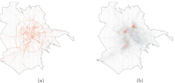
4-1 (a) Car GPS trajectories over 1×1 km grid cells in Rome. (b) Origin-Destination (𝑂𝐷) flow network in Rome with some popular travel locations highlighted. . . 55

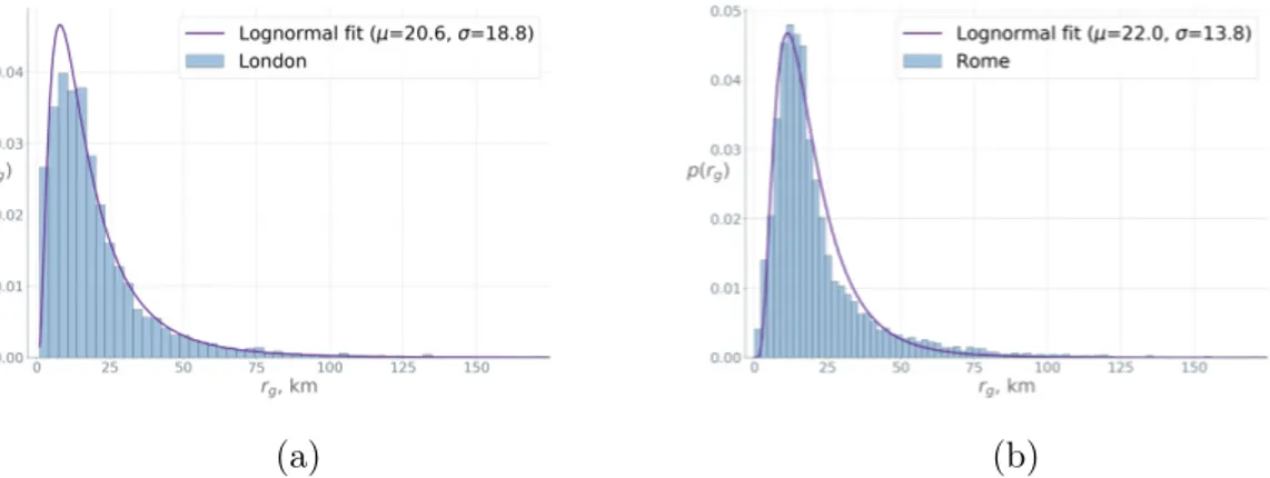
4-2 Empirical distributions of the average radius of gyration per cell in (a) London (b) Rome . . . 56

(10)

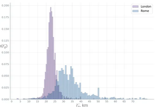
List of Figures List of Figures

4-3 Empirical distributions of the average radius of gyration per cell in

London and Rome. . . 57

4-4 Average street junction betweenness centrality in each 500 × 500m grid cell in London. . . 57

4-5 Examples of node (cell) features in London (a) Average Airbnb listing prices (b) Proportion of grid cell area allotted to industrial activity (c) Number of museums and galleries per grid cell. Darker colours indicate higher values. . . 58

4-6 Examples of node (cell) features in Rome (a) Number of restaurants (b) Proportion of grid cell area allotted to industrial activity (c) Cell area alotted to parking. Darker colours indicate higher values. . . 58

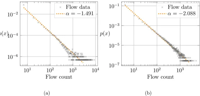
4-7 Log-log plots of the probability distributions of the OD flows fitted with a power-law distribution 𝑝(𝑥) ∝ 𝑥−𝛼 _{with exponents of (a) 𝛼 =} −1.491 in Rome. (b) 𝛼 = −2.088 in London. . . 59

4-8 Total mobility in-flows in (a) Rome (b) London . . . 59

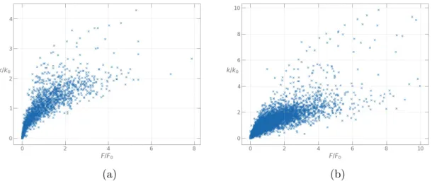
4-9 Correlation between node degree and node total in-flow in the London OD flow network of grid resolution (a) 1000 × 1000 m (b) 500 × 500 m 60 5-1 The urban network of the city of Rome.. . . 76

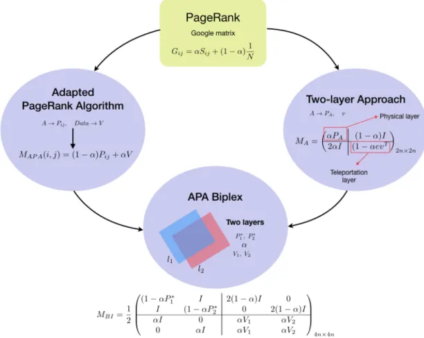
6-1 Schematic representation of the models used to design the APA biplex centrality algorithm . . . 88

6-2 Schematic representation of the APA biplex centrality model . . . 94

6-3 (left) Private car GPS trajectories superimposed on the grid in Rome (middle) Layer 1 of biplex network: Rome OD network with some popular locations highlighted (right) Layer 2 of biplex network: bus connection network. . . 100

6-4 Biplex centrality PGBI for (a) 𝛼1 = 𝛼2 = 0.2 and (b) 𝛼1 = 𝛼2 = 0.8 . 102 6-5 Biplex centrality PGBI for (a) 𝛼1 = 0.3, 𝛼2 = 0.8 and (b) 𝛼1 = 0.8 𝛼2 = 0.3 . . . 102

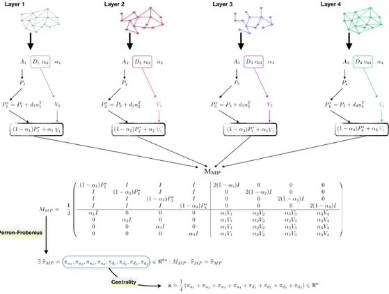
7-1 The APA centrality algorithm for a multiplex network with 4 layers. . 112

7-2 (a) Private car GPS trajectories superimposed on the grid in Rome (b) Rome OD network with some popular locations highlighted. . . . 114

7-3 Rome multiplex mobility network with 4 layers. . . 115

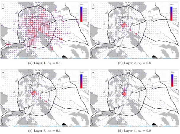
7-4 Multiplex centrality (PGMP) for all the cases analyzed. . . 118

7-5 The multiplex centrality distribution for the cases studied. . . 119

7-6 APA centrality for graphs in layers 1, 2, 3, 4. . . 120

7-7 The 50 most important nodes of all the cases analyzed. . . 121

8-1 Workflow flowchart from raw data input to analysis and visualisation 133 8-2 The APA values for the mobility flow network in Rome (up row) and London (down row) at different times of the day.. . . 134

8-3 (a)-(b) Food service and retail activity APA distributions in Rome, (d)-(e) in London, (c)-(f) Log-log plots of empirical ECDFs in Rome and London at 12:00pm. . . 135

(11)

8-4 Gini (left) and Spatial Gini (right) coefficients during the day for flow only, food service, and retail activity in Rome and London. . . 136

8-5 Gini (left) and Spatial Gini (right) coefficients during the week for flow only, food service, and retail activity in Rome and London. . . . 137

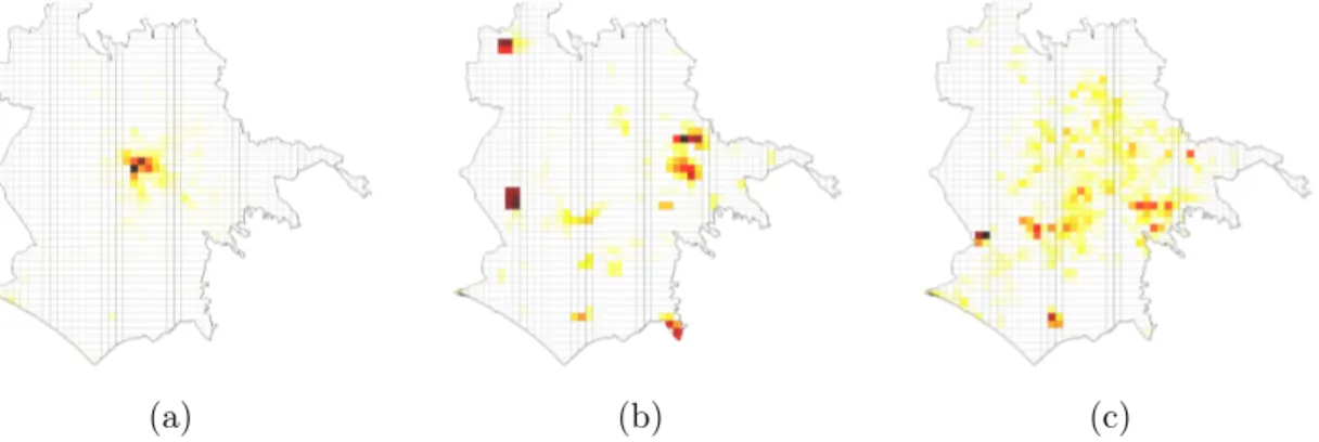
8-6 Hotspot locations with APA values greater than the 50th, 75th, and 90th percentiles in (a) Rome and (b) London. . . 139

8-7 Lorenz curve for a data distribution. . . 140

8-8 Spreading indices over time for various thresholds x* _{in (a) Rome and}

(b) London. . . 140

8-9 Spreading indices for flow only, food services, and retail activity in Rome and London during a typical day. . . 141

8-10 𝑆𝑝𝑟𝑒𝑎𝑑𝑖𝑛𝑔 𝑖𝑛𝑑𝑖𝑐𝑒𝑠 for flow only, food services, and retail activity in Rome and London during the week. . . 142

8-11 Spreading index and time-space spreading index (𝑇 𝑆𝐼) with corre-sponding 95% confidence intervals during a typical day in Rome and London. . . 144

8-12 Tracking the difference 𝑇 𝑆𝐼(x*_{) − 𝜂(x}*₎_{in Rome and London during}

a typical day. . . 145

8-13 Retail APA values at 18:00 in Rome represented with pairwise time-weighted distances between grid cells using multidimensional scaling (𝑀𝐷𝑆). The inset shows the same set of values in geographical space.146

8-14 𝑇 𝑆𝐼 for flow only, food services, and retail activity in Rome and London during a typical day. . . 148

9-1 Estimated parameters of the gravity model for the mobility flows in London . . . 152 9-2 Pearson residuals plotted against fitted means. Rome and London data.153

9-3 The multilayer network representation of the attributed OD network in London. The bottom layer (dark green) captures the observed flow counts between the cells. The top layers (light green) encode different types of relations, such as network distance, average of Airbnb prices, product of population densities, bus or subway network, etc. The gHypE network regression model allows us to explain the impact of these relational layers on the OD flows. . . 156

9-4 gHypE network regression fitted prediction values for (a) London (b) Rome . . . 160

9-5 Speed, network distance, and route factor coefficients over time in (a) London (b) Rome . . . 162

9-6 Population densities, betweenness centrality, residential-to-other, and Airbnb coefficients over time in (a) London (b) Rome . . . 163

9-7 Time, correlation, subway, and bus coefficients over time in (a) Lon-don (b) Rome . . . 164

9-8 Flow only, food services, and retail APA centrality coefficients over time in (a) London (b) Rome . . . 165

9-9 The network distance regression parameter over time under different spatial grid resolutions in London. . . 166

(12)

10-1 The APA centrality values for the mobility flow network in London at different times of the day. . . 171

10-2 (a) Car GPS trajectories over grid cells in London. (b) Origin-Destination (𝑂𝐷) flow network in London. (c) Target flows between a node of interest and every other node. . . 171

10-3 Overview of the neural network model architectures. When predicting the flow for edge 𝑒𝑖𝑗, all three models concatenate the corresponding

edge features 𝑥𝑒

𝑖𝑗, and the node features 𝑥𝑣𝑖, 𝑥𝑣𝑗 of the incident nodes.

The resulting vector is fed into a single fully connected layer. In case of the GNN-based models GNN-geo and GNN-flow, the network also perform graph convolutions on the neighbourhoods of 𝑣𝑖 and 𝑣𝑗 and

computes a weighted sum of both neighbourhood embeddings and the edge embedding. A further set of fully connected layers maps the sum to the predicted flow ˆ𝑦𝑖𝑗. The FCNN model skips the addition

step and does not perform graph convolutions. . . 173

10-4 MAE residuals of flows associated with test nodes (a) GNN-geo. (b) XGBoost. . . 179 B-1 The configuration model illustrated (left) as a typical edge rewiring

exercise and (right) as analogous to the urn problem. In the first case, in order to obtain a new multi-edge, first an out-stub (𝐴, ·) is sampled for rewiring, then an in-stub is sampled uniformly at random from those available. If each possible combination of out- and in-stubs is represented as a ball, we get the urn problem without replacement. In this setting, the probability of observing a multi-edge (𝐴, 𝐵) is three times as high as that of observing a multi-edge between (𝐴, 𝐷) and 1.5 times as high as that of observing a multi-edge between (𝐴, 𝐶) in both the edge rewiring and the urn schemes. . . 217

B-2 Edge propensities driving the selection process in the configuration model. As opposed to the conventional configuration model, in this case the stubs are not sampled uniformly at random as in Figure B-1. Once an out-stub has been sampled, each in-stub is then described by a propensity Ω𝑖𝑗 of being sampled to form the new multi-edge.

This results in the odds of wiring the out-stub (𝐴, ·) to the node D being higher than that of B because of a very large edge propensity Ω𝐴𝐷,despite node B having three times more in-stubs than node D. . 217

(13)

List of Tables

5.1 Fifty first values of the APA centrality for different 𝛼 values . . . 78

5.2 Fifty first values of the APAM2 centrality for different 𝛼 values . . . 79

5.3 Fifty first values of the CVP centrality. . . 80

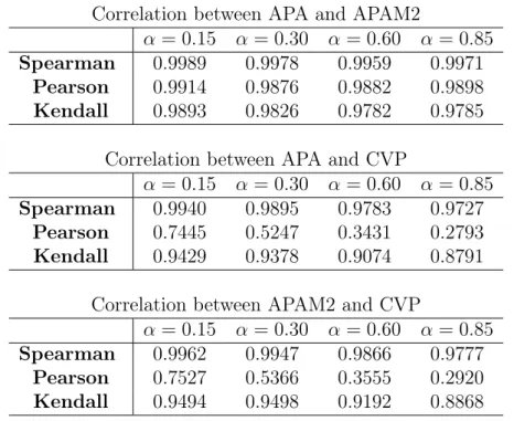
5.4 Pearson, Spearman and Kendall correlation coefficients. . . 81

6.1 The first 25 most central nodes for the studied numerical cases. . . . 104

9.1 Comparison of gHypE multilayer regression performance against base-line methods . . . 160

9.2 MLE coefficients of the gHypE multilayer regression model in London 161 10.1 Comparison of model performance in terms of mean absolute error grouped by flow magnitude. . . 179

10.2 Comparison of model performance in terms of MAPE, SSI, CPL, and CPC. . . 180

A.1 Summary of the OD network datasets . . . 212

A.3 Node attributes of the500×500m OD network . . . 212

(14)

"If you do not care about networks,

the networks will care about you, anyway. For as long as you want

to live in society, at this time and in this place, you will have to deal

with the network society."

Manuel Castells, 2001

Chapter 1 Introduction

Let me introduce the reader to the topic of my PhD work in the Data Science PhD program jointly held byScuola Normale Superiore of Pisa(SNS),University of Pisa

(UniPi),National Research Council(CNR),Sant’Anna School of Advanced Studies

(SSSA), andIMT School for Advanced Studies Lucca (IMT).

1.1 What is urban data science?

The origins of urban data science can be tracked to the field of urban analytics which, broadly speaking, develops, utilises and exploits a set of analytical methods and big data to study, understand and predict properties and features of urban environments, formalised as urban systems [236]. However, overly focused on data analysis of huge urban data streams collected from various sources in the city (see Section 2.1.2), urban analytics often lacks a firm methodological foundation and clarity about research paradigms. Given this shortcoming and the unprecedented growth in data-informed research on cities in the past 20 years, Michael Batty calls for the need "to go beyond data analysis per se" and establish a theory of the urban -city science - aimed at understanding and explaining spatial and temporal variations of urban phenomena [31].

In [199], the authors establish the term "urban data science" by extending ur-ban analytics and city science to require the incorporation of both quantitative and qualitative methods, and, most importantly, a clear research paradigm and a

(15)

dia-Chapter 1. Introduction 1.2. What is this thesis about?

logue with other established scientific fields from which to borrow and with which to intertwine our understanding of cities as complex systems.

This aspect is particularly important for the present thesis, as it aims to explore, model, and understand the complex relationships between urban socio-economic characteristics and urban mobility, and will attempt to accomplish this via the scientific apparatus of network science.

In what follows, I will provide a short comprehensive excursion into the essence of this work with which the reader will be offered a road map of the motivation, research questions, methodology, main contributions, and results of this PhD thesis.

1.2 What is this thesis about?

If I were to outline what the present PhD thesis contributes to and what it is essentially about in just a few paragraphs, it would be:

I

What is this PhD thesis essentially about?

The bulk of research in City Science - a computational understanding of urban systems - can be said to follow two main trajectories: that of urban structure and urban mobility [30]. The former studies the spatial organisation and mor-phology of the physical infrastructure, urban space, and the location choices of firms and individuals - also known as urban economics. The latter, on the other hand, studies the individual and collective movement patterns in cities to inform urban and transportation planning.

This thesis attempts to bridge the two trajectories, presenting a methodology for studying the intricate relationships between urban structure and urban mobility through the lens of network science.

Classical urban geography treats urban phenomena as spatial processes in which the relations of urban spaces and locations among each other is lim-ited to so-called spillover effects typically decaying with distance [200]. Urban space is primarily understood in geographical or temporal space, with a lo-cally determined part-to-whole relationships to the city. A major conceptual

(16)

Chapter 1. Introduction 1.2. What is this thesis about?

II

view underpinning the present thesis is whether the city can be meaningfully represented in relational space, and, if so, whether this representation can help us extract new kinds of knowledge about cities as systems and reevalu-ate part-to-whole relationships in the city. In particular, this thesis models the city as a network of mobility flows encoded with origin-destination (OD) matrices, augmented with attributes describing network nodes - city locations (e.g., population density, number of restaurants, real estate prices, etc.) and edges - the various relationships between them (e.g., road distance, travel time, public transport connections, etc.). This attributed urban mobility network is then studied from two methodological viewpoints:

• Network centrality measures

• Urban flow modelling and prediction

First, new network centrality measures based on the Google PageRank algo-rithm are presented. Just like how Google ranks web pages based on queries, urban planners or policy makers are given the opportunity to "search" the ur-ban network based on specific criteria of desired urur-ban attributes to study the spatio-temporal characteristics of city locations and to inform urban planning and policy making. Then, rankings obtained from the introduced algorithms are used to enhance the modelling and prediction of urban mobility flows. This is achieved via two novel approaches presented in the thesis:

• Statistical random graph regression, in which the observed urban mobility network is considered a realisation from an ensemble of ran-dom graphs and is regressed on socio-economic attributes describing the urban environment with the aim of explaining the effect each attribute has on the mobility flows.

• Graph Neural Networks for predicting flows to/from a specific lo-cation of interest in a city. Imagine a developer aims to build a new commercial center at a given location in the city, knowing the socio-economic attributes of that location in advance (i.e., type of activity, retail volume, parking area, etc.). Can we predict the mobility to/from

(17)

Chapter 1. Introduction 1.3. Thesis Structure

III

that location, given the attributes of the project location and the rest of the mobility network?

Thus, this thesis presents a network-oriented methodology to describe, model, analyze, and predict spatio-temporal aspects of urban mobility flows.

1.3 Thesis Structure

The present PhD thesis is a cumulative thesis. The individual thesis chapters are essentially modified versions of papers published in the course of three years of the PhD program.

In what follows, the thesis structure and a brief synoptic outline of each individual chapter are presented.

Chapter 2 - Background In this Chapter, we prepare ground for the subsequent body of work by motivating why studying cities and urban mobility is impor-tant, by introducing core concepts we are going to work with, and by providing an extensive review of literature in urban structure and urban mobility, and baseline techniques and models we will build upon and develop.

Chapter 3 - Thesis Objectives In this Chapter, we define the objectives of our work and formulate the research questions we will attempt to answer.

Chapter 4 - Data Here we describe in detail the methodology and process of building the urban mobility network dataset from private car GPS trajecto-ries, augmented with socio-economic attributes describing city locations from various open sources. We explore the dataset, discuss its main features, and set a common ground to be referred to and used by the main body of work represented in the remaining chapters of this thesis.

Chapter 5 - Adapted PageRank and Eigenvector Centrality In this Chap-ter, we introduce the conceptual framework for centrality measures based on the Google PageRank and discuss the motivation and importance of such cen-trality measures in an urban context. This Chapter is a modified version

(18)

of our paper "Analysis and comparison of centrality measures applied to ur-ban networks with data" in which we present new centrality measures based on the Google PageRank and eigenvector centralities for networks augmented with node attributes, provide a comparative analysis, and apply the discussed measures on the constructed OD flow network in Rome. The presented algo-rithms offer the possibility to choose the relative importance of the attribute data with respect to the network topology in computing the rankings, thus providing the urban planner with a high flexibility.

Chapter 6 - APA centrality for Biplex urban networks In this Chapter, we build upon the Adapted PageRank Algorithm presented in the previous Chap-ter 5, by extending it to a biplex mobility network setting. This Chapter is a modified version of our paper "A centrality measure based on the Adapted PageRank Algorithm for multiplex networks with data" which modifies and enhances the previously introduced APA centrality to a multiplex network with the possibility to control for the importance of node attribute data with respect to the network topology in each of the network layers. The presented algorithm is then applied to a case study of the Rome urban OD network with mobility flow and bus connection layers, where different parametrisations of the relative importance of attribute data with respect to the flow network topology are compared.

Chapter 7 - APA centrality for Multiplex urban networks This Chapter is a conceptual follow-up of the previous Chapter 6 which introduced the APA centrality for biplex mobility networks, and naturally extends it to a multi-layer setting with the possibility to consider many kinds of relations between city locations at the same time. This Chapter is a modified version of our pa-per "Understanding mobility in Rome by means of a multiplex network with data" in which we apply the presented APA centrality algorithm for multi-plex networks to the same Rome OD flow network extended to include subway connections and topologically short travel distances as additional network lay-ers. Different cases of attribute data importance in each of the layers are then

(19)

considered and the possibilities of such a multilayer network approach are highlighted. We will use the rankings obtained from this algorithm to enhance the explanatory and predictive models in Chapters 9 and 10.

Chapter 8 - Spatio-temporal APA centrality In this Chapter, we build upon the APA centrality paradigm introduced in Chapter 5, and explore spatio-temporal characteristics of the distribution of APA centrality values in cities. In particular, this Chapter is a modified version of our paper "Ranking places in attributed temporal urban mobility networks" in which we apply the APA centrality introduced in previous chapters to temporal urban OD flow networks in Rome and London. We introduce several metrics to capture the spatial dis-tribution of "hotspots" with high centrality values across different hours of the day and days of the week in both cities, look at how different socio-economic attributes affect the spatio-temporal behaviour of "hotspots", and provide a comparison among the two cities. The Chapter both presents a methodology for studying urban space with its socio-economic characteristics within a net-work paradigm and a practical net-workflow for building and monitoring mobility in a city with specific simple metrics.

Chapter 9 - Explaining mobility from urban attributes We place this Chap-ter within the paradigm of human mobility modelling by considering the at-tributed urban mobility network as a multilayer network with each attribute - both node and edge, including the APA centrality rankings computed in previous chapters - transformed into dyadic relationships and considered as a separate layer in the network. Within this framework, the OD flow layer is considered as a realisation from a particular family of statistical random graphs. A regression model respecting the network topology is then proposed, in which the OD flow layer is regressed on the dyadic attribute layers, offering the possibility to explain the impact each attribute layer has on the observed urban OD flow network. A temporal regression setting is further presented, with results compared for Rome and London.

(20)

Chap-Chapter 1. Introduction 1.3. Thesis Structure

ter is a modified version of our "Learning Mobility Flows from Urban Features with Spatial Interaction Models and Neural Networks" paper in which we propose several neural network-based architectures, including Graph Neural Networks (GNN) for predicting mobility flows to/from a specific city location, the socio-economic attributes of which are known in advance. We show how the proposed models significantly outperform classical mobility models and more recent machine learning approaches, and demonstrate the impact of the previously computed APA centralities on the prediction accuracy.

Chapter 11 - Conclusion This Chapter concludes the PhD thesis by summaris-ing the formulated research questions and the methodology proposed in the different Chapters for tackling these, discussing the main results and findings, highlighting the advantages of the presented techniques, pointing out draw-backs and shortcomings, and sketching the directions for improvement and future work.

(21)

"If a man who can’t count finds a four leaf clover, is he lucky?"

Stanislaw Lem

Chapter 2 Background

2.1 Introduction and motivation

2.1.1 Why cities?

Along with the agricultural revolution, the first city-like settlements came to be approximately 10,000 years ago [184] and witnessed unprecedented growth with the industrial revolution. The first city to reach 1,000,000 inhabitants was London, at the heart of the industrial revolution, at the onset of the 19th century. This un-leashed the further spread through the end of the 19th _{and the 20}th _{centuries to} other parts of the world. However, while western countries are already largely ur-ban (in 2017, the US population was 82% urur-ban, Australia’s 86%, and the majority of the countries in the EU hosted around 80% of their population in cities [115]), the significant part of ’rapid urbanisation’ takes place in developing countries. 2005 marked the year in which it was estimated by the U.N. that more than 50% of the world population was inhabiting in cities [186]. It is beyond doubt that urbanisation is not a contingent phenomenon in history, and that the impact cities are going to have on the world is only expected to grow. In fact, the importance of cities in the modern world is already enormous.

First, they play a disproportionately large role in the world’s economy. A 2011 report by McKinsey revealed that while the USA and India had respectively 79% and 19% of urban population, their contribution to their countries’ respective GDP

(22)

Chapter 2. Background 2.1. Introduction and motivation

was 85% and 39%. NASA data show that urbanised areas cover 6% of the total land surface area in the world, comparable in size to the whole area of the European Union. Notwithstanding their relatively small spatial trace, cities have a consider-able environmental impact. The United Nations reported in 2016 that cities were responsible for 74% percent of the world’s CO2 emissions.

Representing but the tip of the iceberg, the above-mentioned should suffice to con-vince anyone of the importance to study and understand cities if we want to make the world we built for ourselves a better place. The unprecedented explosion of urbanisation in developing countries poses significant challenges. Both the cause as well as the solution of some of the most pressing problems in the world unarguably lie in cities. By improving the way cities function we can possibly have a dramatic impact on people’s lives. In order to do so however, we need to understand how they function first.

2.1.2 Why data?

The fundamental game changer in research on cities is data. We now have at our availability huge amounts of data pertaining to virtually all aspects of urban life. Data about many different processes is available at various scales.

At short time scales, we have human mobility data originating from call detail records (CDR) that contain information on the location of individuals at the moment of making a call. Until relatively recently this kind of data was mainly obtained by surveys that had limitations with respect to time and space, whereas CDR or automobile GPS data give a much more precise and real-time overview of mobility in cities. Moreover, the use of Radio-frequency identification (RFID) in subway, bus, and private vehicle transport modes enhance this type of datasets and the growing set of different sensors in urban environments measuring, for instance, air pollution offer the possibility to extend our understanding and modeling of urban mobility.

At larger time scales of several months to a year, there is socioeconomic data on such aspects as the income-location relationship, the spatio-temporal change in real-estate prices, etc. Finally, at a very long time scale, the digitization of historical documents such as maps offers the opportunity to study the long-term evolution and

(23)

change of urban infrastructure. All the mentioned types of data are indispensable in the process of modelling and studying cities and the revelation of the major forces that propel their evolution.

Another crucial issue has to do with the accuracy of the mentioned new datasets. It is necessary to test and compare them with more conventional methods of ob-taining socioeconomic data, for example surveys. In [164] the authors investigated the relationship between various sources of data concerningOrigin-Destination flow

(OD) matrices1 _{describing mobility in Spanish cities with data obtained from}

Twit-ter, CDRs, and census data. They showed a valid consistency between the different datasets. The study showed the importance of working with a multitude of different data sources, allowing for cross-checking the obtained results (Figure 2-1a).

(a)

(b)

Figure 2-1: (a) Correlations between data sources [164]. (b) The reachability within 30 minutes by foot, bycicle, and car in the city of Marseille, France [196].

2.1.3 Why mobility?

Mobility is undoubtedly a critical phenomenon in urban environments. In fact, it can be considered as one of the most important mechanisms underlying the structure and dynamics of contemporary cities. Indeed, cities are places where intensive buying,

(24)

selling or exchanging goods is taking place, where individuals commute to work or meet with other individuals. An obvious means to achieve all this is transportation. Here is where technology enters the picture via the average and maximum velocity of different transportation modes. This average velocity has increased considerably as technology evolved and modified the spatial organization of cities. For instance, as we can see in Figure2-1b, the reachability of an individual depends on the trans-portation mode. For a pedestrian, the reachability horizon is typically isotropic and small, whereas the car permits a wider yet anisotropic exploration of space due to the existing infrastructures. The described correlation between the spatial organi-sation of a city and the available technology at the time has been demonstrated by [18] for American cities. The authors of the study show how many big cities, such as Denver, grew around rail stations which unleashed the development of central business districts. Later automobile-era cities such as Dallas, on the other hand, display a spatial structure primarily conditioned by the highway system.

In terms of mobility, the traditional city center can be regarded as the location that mimimises the average distance to all other locations in the city. As a natural consequence, it has thus historically attracted businesses and residences, leading to competition for the limited space among individuals or firms, which gave rise to the real-estate market. There exists also a well-studied relationship between land-use and accessibility, as was shown half a century ago in [120], and it can be expected that new datasets will certainly offer new possibilities to precisely portray the rela-tion between these and other important factors.

It is certainly neither reasonable nor possible to make an all-encompassing re-view on all available studies on mobility and our focus in this thesis will be rather on certain specific points. We will firstly describe the general features of urban mobility considering the central quantity in these studies - the origin-destination (𝑂𝐷) matrix - and discussing how to extract useful information from it. Next, we will formulate hypotheses about how to approach the intricate relationships between urban mobility and urban spatial structure.

(25)

2.1.4 Why spatial structure?

Morphological aspects of the city, such as the quantitative description and compari-son of cities according to their density landscape, spatial organisation, polycentricity, or the clustering variation of their activity centers, have already been studied for a long time in urban geography and spatial economy [18, 39, 261, 213, 233, 255,

116,38, 159]. However, there seems to be a lack of precision when dealing with the fundamental object of our study: the city. Despite some efforts from urban geogra-phers to build a common ground as to the definitions of a city [219], we still lack an univocal, theoretically sound definition of what a city is. And this is problematic, since statistical results stem from what is deemed as the most suitable definition of the city at the time and context of the study. This in turn influences the ability to generalise research results on cities. If we aim to obtain robust empirical results, compare the results obtained in different countries, we would need to begin think-ing about the definition of the system of our study. With a definition of the study object more or less set up, a usual starting point towards our goal of understanding how cities are spatially structured is to study how objects are scattered within it. By objects it is meant buildings, roads, economic activities, but most importantly, people.

The way the distribution of objects in space is traditionally studied is via the study of densities. With a growing scale, however, density profiles become too com-plicated to comprehend and work with. Several attempts have been made towards approaching this problem in the field of spatial statistics as well as urban form [233, 261, 182, 264]. Authors in them attempt to resolve this issue by proposing simple measures that extract a single index from the density profile. A paramount example is the Moran’s 𝐼 [182] defined as:

𝐼 = 𝑁 𝑊 ∑︀ 𝑖 ∑︀ 𝑗𝑤𝑖𝑗(𝑥𝑖− ¯𝑥)(𝑥𝑗 − ¯𝑥) ∑︀ 𝑖(𝑥𝑖− ¯𝑥)2 , (2.1)

where 𝑁 is the number of spatial units indexed by 𝑖 and 𝑗; 𝑥 is the variable of interest; ¯𝑥 is the mean of 𝑥; 𝑤𝑖𝑗 is a matrix of spatial weights with zeroes on the diagonal (i.e., 𝑤𝑖𝑖 = 0); and 𝑊 is the sum of all 𝑤𝑖𝑗. The Moran’s 𝐼 measures the

(26)

Figure 2-2: Measure of the spatial autocorrelation among spatial units degree to which similar objects in space tend to cluster together. Its values range from -1 to 1, with -1 corresponding to perfect clustering of dissimilar values, with +1 to perfect clustering of similar values, and with 0 indicating no autocorrelation (perfect randomness, Figure 2-2). It is worth mentioning that Morans’s 𝐼 index is related to the "First Law of Geography" which states that "everything is related to everything else, but near things are more related than distant things." [257]

Another example of a single index, in this case measuring the heterogeneity of population densities in the city is the modified Gini coefficient [264]:

𝐺𝛼 = ∑︁ 𝑖,𝑗∈𝛼|𝑃𝑖− 𝑃𝑗| 2𝑛𝛼 ∑︁ 𝑖∈𝛼𝑃𝑖 , (2.2)

where the sums run over all 𝑛𝛼 cells covering the surface of the municipality 𝛼. The Gini coefficient is predominantly used in Economics [110, 111], and was originally proposed to measure the inequality degrees in distributions of wealth and income but has been modified in [264] to capture the level of heterogeneity of population densities. It takes on the value of zero for a city in which the population is uniformly distributed in all grid cells, and is maximum for an extremely concentrated city, with the total population residing in a single grid cell.

A single index is nonetheless too simple to accurately capture complex spatial relationships. For example, as we can see in Figure2-3, the spatial organisation of the population densities can be reshuffled to obtain different layouts with exactly the same Gini coefficient, demonstrating the inability of this index to capture how

(27)

values are organised in space. Although the authors go on to introduce another index compensating for this shortcoming, the example demonstrates the need for more sophisticated representations. Hence, what is needed is rather a meso-scale measure, somewhere between the micro-scale representation (the density profile itself) and the macro-scale representation (a single index summarising the density profile). We conjecture that since ’centers’ are themselves a meso-scopic system, their working definition ought to emerge readily from such a representation.

(a) (b)

Figure 2-3: (a) The population distribution in Paris in 2013 and different distribu-tions with exactly the same Gini [264]. (b) Illustration of a trajectory flow map, a dynamic graph of aggregated traffic flows constructed from trajectory data. The presented example is based on bus passenger trajectories obtained in Brisbane, Australia [143].

Until relatively recently these quantitative characterisations of urban form were primarily based on transport surveys, census data, and remote sensing data, all al-lowing for a fine spatially granular population density and land use estimation, but lacking the same granularity in the temporal dimension. It should be noted here that early studies in urban geography [96,114] estimated population density at different hours of the day using transport surveys and could trace the morphological and socioeconomic evolution of urban areas during the day. In addition, various traffic surveys in cities around the world have provided an overall outline of the temporal dimension of urban mobility.

However, given their rather coarse temporal resolution and the absence of ap-propriate data, these studies were not able to study some crucial questions related to dynamical characteristics of the spatial organisation of cities: how does the city’s population and/or activity density profile change throughout the day? What is the

(28)

spatial distribution of the city’s hotspots at different times of the day? How are these hotspots or points of interest (POI) spatially organized? Is there any hierar-chy in the spatial organization of hotspots, and if so, is it robust through time? Is there some kind of characteristic distance(s) characterizing the invariant core of a city?

Given the importance and challenges associated with the study of the spatial structure of cities and its non-trivial relationships with urban mobility, this the-sis will attempt to approach the above-mentioned issues from a complex network theoretical perspective.

2.1.5 Why complex networks?

The science of networks has been witnessing a rapid development in recent years: the metaphor of the network, with all the power of its mathematical devices, has been applied to complex, self-organized systems as diverse as social, biological, tech-nological and economic, leading to the achievement of several unexpected results in the seminal works of Barabási, Strogatz, Pastor-Satorras and others [15, 249, 209]. Our understanding of spatial networks that are omnipresent in biological, techno-logical and infrastructural systems [181, 27] has seen an unprecedented progress in the recent years. However, notwithstanding a significant amount of research on these kinds of networks, in disciplines covering among others mathematics, physics, biology, and geography, their topological, structural and dynamical properties are not yet completely understood. These networks have proven to be relevant in urban systems [55, 40, 206, 29,26] where the studies of their structure and topology have revealed particular characteristics of cities as well as shown remarkable statistical properties such as scale invariant patterns across various urban spaces [112,41,138]. The street network with its geometry is of particular importance, providing the res-idents functional connections for navigating various components of the urban area. Different street patterns allow for different levels of efficiency, accessibility, and util-isation of infrastructure [137, 72, 270, 140]. Thus, structural properties of street networks have been the object of several studies [152, 268, 173, 248].

(29)

spa-Chapter 2. Background 2.1. Introduction and motivation

tial distributions, urban sprawl and the evolution of urban networks, are but a few of the important mechanisms that have been systematically studied but that we now hope to comprehend quantitatively. The various network models can be thought of as a simplified abstracted view of cities, which capture important parts of their structure and organization [243] and contain the possibilities to unlock the underlying universal processes behind their formation and development. Apart from modelling the street network as a graph, thus restricting oneself to its planar proper-ties, other network approaches capturing various kinds of relationships, particularly mobility, between different parts of the urban area, have also been experimented with [143, 229, 308, 250, 163, 134, 302, 292] (Figure 7-2). Extracting similar pat-terns among cities is one of many ways towards the identification of these conjectured underlying processes. One important question, for example, boils down to the mech-anisms behind bottom-up ’organic’ patterns - which evolve under local constraints - and whether and how they are different from the top-down, planned patterns by a central authority which appear under large scale constraints. This direction of research is by no means new [283, 28], but the recent unprecedented increase of available data such as historical or contemporary digital maps [198,247] and tempo-rally granular mobility data allow to proceed with large scale cross-sectional models and their evolution in both short and longer period of time (Figure2-3b).

Some types of networks, like street and road networks, are now more or less adequately described [136,228,217, 217,77,67, 73]. Because of spatial constraints, they show a peaked degree distribution, large assortativity and clustering coefficient, and the most revealing and valuable characteristic is the spatial distribution of a graph-theoretical measure called betweeenness centrality (see section 2.2.1)

A crucial aspect is that the main instrument for mathematically representing a network - the adjacency matrix - is not sufficient to capture all relevant information about the system. In particular, the spatial distribution of node geometry plays a critical role. A classification of cities according to their street network should then rely on both topology and geometry.

However, the particular relationships between the street network, differently con-structed mobility networks along with their evolution over time, and the actual

(30)

Chapter 2. Background 2.2. Network centrality measures

physical patterns of the city are non-trivial and poorly understood. We believe that results in this direction would open up the possibility for devising methods to the challenging problem of urban mobility prediction and transfer learning to cities with scarce data. Although some results, primarily in traffic and travel de-mand forecasting [267, 295] and graph-based transfer learning have been achieved [123, 133, 160], we still lack systematic methods for mobility-informed prediction of urban spatio-temporal dynamics. This thesis will attempt to tackle this critical problem.

(a) (b)

Figure 2-4: (a) Map and network of the city of Murcia, Spain. [1] (b) The commu-nity structure of San Francisco urban regions. Different color represents different traffic community, the spatial partition among the four communities are quite obvious [250].

2.2 Network centrality measures

A crucial set of instruments indispensable to the study of most kinds of networks are network centrality measures. Centrality measures serve to quantify the idea that in a network some nodes are more important (central) than others.

As mentioned before, the science of networks has witnessed a dramatic increase in its applications in systems spanning social, economic, technological and other dis-ciplines. In particular, the issue of centrality in networks has remained pivotal, since its introduction in a part of the studies of humanities named structural sociology [274]. The idea of centrality was first applied to human communication by Bavelas [32] who was interested in the characterization of the communication in small groups

(31)

of people and assumed a relation between structural centrality and influence and/or power in group processes. Since then, various measures of structural centrality have been proposed over the years to quantify the importance of an individual in a social network [32]; and the issue of centrality has found many applications also in biology and technology. Currently, centrality is a fundamental concept in network analysis though with a different purpose: while in the past the role and identity of central nodes were investigated, now the emphasis is more shifted to the distribution of centrality values through all nodes. Centrality, as such, is treated like a shared re-source of the network community, like wealth in nations, with the focus being on the homogeneity and/or heterogeneity of distributions [15]. In urban planning and de-sign, as well as in economic geography, centrality, though under different terms like accessibility, transport cost or effort, has entered the scene stressing the idea that some places are more important than others because they are more central [278]; all these approaches have been following a primal representation of spatial systems, where punctual geographic entities - street intersections, settlements - are turned into nodes and their linear connections - streets, infrastructures - into edges. A pio-neering discussion of centrality as inherent to urban design in the analysis of spatial systems has been successfully operated after Hillier and Hanson seminal work on cities [125] since the late 1980s. Space Syntax, the proposed methodology of urban analysis, has been raising growing evidence of the correlation between the so-called integration of urban spaces, a closeness centrality in all respects, and phenomena as diverse as crime rates, pedestrian and vehicular flows, retail commerce vitality and human way-finding capacity [124]. The Space Syntax approach follows a dual rep-resentation of street networks where streets are turned into nodes and intersections into edges. An outcome of the dual nature of Space Syntax is that the node degree is not limited by physical constraints, since one street has a conceptually unlimited number of intersections; this property makes it possible to witness the emerging of power laws in degree distributions [136, 228] that have been found to be a distinct feature of other nongeographic systems [15, 249, 209, 23]. On the other hand, the dual character leads Space Syntax to the abandonment of metric distance: a street is one node no matter its real length. Metric distance, conversely, was the core of

(32)

most territorial studies [231] and is a key ingredient of spatial networks.

When dealing with urban street patterns, centrality has been investigated in re-lational (topological) networks only, neglecting a fundamental aspect of the system as the geography. In the majority of past approaches a city is transformed into a spatial graph by mapping the intersections into the graph nodes and the roads into links between nodes. By using a set of different centrality indices (multiple centrality assessment [77,76]), extended or defined on purpose for spatial graphs, it is possible to spot the relevant places of a city. By relevant places it is meant places closer to other places (closeness centrality), places that are structurally made to be traversed (betweenness centrality), places whose route to other places deviates less from the virtual straight route (straightness centrality), and places whose deactiva-tion affects the structural properties of the system (informadeactiva-tion centrality). Apart from the mentioned purely structural centrality measures aaplied to urban networks, attention has recently been drawn towards more sophisticated centrality concepts allowing for integration of valuable information about different places in the city in measuring their respective centralities. Such measures include, among others, the modified Google PageRank and Eigenvector centralities (see section 2.2.2). More-over, by investigating how centrality is distributed among the nodes of the graph, how the different centrality indices are correlated, and how they evolve in the tem-poral dimension, it is possible to study urban dynamics and also characterise classes of cities [76].

2.2.1 Multiple centrality assessment

The multiple centrality assessment relies on three basic principles [77,76] as follows: label=(0) primal graphs, rather than dual;

lbbel=(0) metric distance, rather than topological;

lcbel=(0) many centrality indices, rather than mainly closeness

The following is a list of common centrality measures we. The definitions are given in terms of an undirected, weighted graph 𝐺, of 𝑁 nodes and 𝐾 edges. The

(33)

Figure 2-5: (a) Degree distribution of degrees for the road network of Dresden. (b) The frequency distribution of the cells surface areas 𝐴 obeys a power law with exponent 𝛼 ≈ 1.9 (for the road network of Dresden) [152].

graph is described by the adjacency 𝑁 × 𝑁 matrix 𝐴, whose entry 𝑎𝑖𝑗 is equal to 1 when there is an edge between 𝑖 and 𝑗 and 0 otherwise, and by a 𝑁 × 𝑁 matrix 𝐿, whose entry 𝑙𝑖𝑗 is the value associated to the edge: for planar street networks usually the metric length of the street connecting 𝑖 and 𝑗; for mobility networks usually the amount of traffic flowing from 𝑖 to 𝑗 in a fixed amount of time.

Degree centrality

Degree centrality, 𝐶𝐷_{, is the simplest definition of node centrality. It is based on} the idea that important nodes have the largest number of ties to other nodes in the graph. The degree centrality of 𝑖 is defined as [274, 193, 105]:

𝐶_𝑖𝐷 = ∑︀𝑁 𝑗=1𝑎𝑖𝑗 𝑁 − 1 = 𝑘𝑖 𝑁 − 1, (2.3)

where 𝑘𝑖 is the degree of node 𝑖, i.e., the number of nodes adjacent to 𝑖. Degree centrality is not particularly interesting in primal urban networks where node degrees are limited by geographic constraints and show a peaked distribution. For example, in a study of 20 German cities, Lämmer et al. [152] showed that most nodes have four neighbors (the full degree distribution is shown in Figure 2-5) and that the degree rarely exceeds 5 for various world cities [61].

(34)

Closeness centrality

Closeness centrality, 𝐶𝐶_{, measures to which extent a node 𝑖 is near to all the other} nodes along the shortest paths, and is defined as [274, 230]:

𝐶_𝑖𝐶 = ∑︀𝑁 − 1 𝑗∈𝐺,𝑗̸=𝑖𝑑𝑖𝑗

, (2.4)

where 𝑑𝑖𝑗 is the shortest path length between i and j, defined, in a weighted graph, as the smallest sum of the edges length throughout all the possible paths in the graph between 𝑖 and 𝑗.

Betweenness centrality

Betweenness centrality, CB, is based on the idea that a node is central if it lies between many other nodes, in the sense that it is traversed by many of the shortest paths connecting couples of nodes. The betweenness centrality of node i is [105,146]:

𝐶_𝑖𝐵 = 1 (𝑁 − 1)(𝑁 − 2) ∑︁ 𝑠̸=𝑡∈𝑉 𝜎𝑠𝑡(𝑖) 𝜎𝑠𝑡 , (2.5)

where 𝜎𝑠𝑡 is the number of shortest paths going from nodes 𝑠 to 𝑡 and 𝜎𝑠𝑡(𝑖) is the number of these paths that go through 𝑖 [104].

Straightness centrality

Straightness centrality, 𝐶𝑆_{, originates from the idea that the efficiency in the} com-munication between two nodes 𝑖 and 𝑗 is equal to the inverse of the shortest path length 𝑑𝑖𝑗 [156]. The straightness centrality of node 𝑖 is defined as

𝐶_𝑖𝑆 = 1 𝑁 − 1 ∑︁ 𝑗∈𝐺,𝑗̸=𝑖 𝑑𝐸𝑢𝑐𝑙_𝑖𝑗 /𝑑𝑖𝑗, (2.6) where 𝑑𝐸𝑢𝑐𝑙

𝑖𝑗 is the Euclidean distance between nodes 𝑖 and 𝑗 along a straight line, and there has been adopted a normalization proposed for geographic networks [265]. This measure captures the extent to which the connecting route between nodes 𝑖 and 𝑗 deviates from the virtual straight route.

(35)

Information centrality

Information centrality, 𝐶𝐼_{, is a measure introduced in [}₁₅₈_{], and relating a node} importance to the ability of the network to respond to the deactivation of the node. The network performance, before and after a certain node is deactivated, is measured by the efficiency of the graph 𝐺 [156, 157]. The information centrality of node 𝑖 is defined as the relative drop in the network efficiency caused by the removal from 𝐺 of the edges incident to 𝑖,

𝐶_𝑖𝐼 = 𝛿𝐸

𝐸 =

𝐸[𝐺] − 𝐸[𝐺′]

𝐸[𝐺] (2.7)

where the efficiency of a graph G is defined as

𝐸[𝐺] = 1

𝑁 (𝑁 − 1) ∑︁ 𝑗∈𝐺,𝑗̸=𝑖

𝑑𝐸𝑢𝑐𝑙_𝑖𝑗 /𝑑𝑖𝑗 (2.8)

and where 𝐺′ _{is the graph with 𝑁 nodes and 𝐾 − 𝑘}

𝑖 edges obtained by removing from the original graph 𝐺 the edges adjacent to node 𝑖. An advantage of using the efficiency to measure the performance of a graph is that 𝐸[𝐺] is finite even for disconnected graphs [76].

As shown in [76], Closeness, straightness, and betweenness centrality distribu-tions, where the cumulative distribution 𝑃 (𝐶) is defined as

𝑃 (𝐶) = ∫︁ +∞ 𝐶 𝑁 (𝐶′) 𝑁 𝑑𝐶 ′ , (2.9)

where 𝑁(𝑐) is the number of nodes with centrality equal to 𝐶, are quite similar in both self-organized and planned cities, despite the diversity of the two cases in socio-cultural and economic terms could not be deeper. On the other hand, the information centrality distributions notably differentiate self-organized cities from planned ones, being broad-scale (power law) in the first case, and single-scale (ex-ponential) in the second case (Figure2-6b).

(36)

(a) (b)

Figure 2-6: a. Thematic color map representing the spatial distributions of cen-trality in Cairo, an example of a largely self-organized city. The four indices of node centrality, (a) closeness 𝐶𝐶_{, (b) betweenness 𝐶}𝐵_{, (c) straightness 𝐶}𝑆_{, and} (d) information 𝐶𝐼, used in the MCA, are visually compared over the primal graph. Different colors represent classes of nodes with different values of the cen-trality index. The classes are defined in terms of multiples of standard deviations from the average, as reported in the color legend. b. Cumulative distributions of (a) closeness 𝐶𝐶_{, (b) betweenness 𝐶}𝐵_{, (c) straightness 𝐶}𝑆_{, and (d) information 𝐶}𝐼 for three planned cities, Los Angeles, Richmond, and San Francisco. The dashed lines in panels (b) are Gaussian fits to the betweenness distributions, while the dashed lines in panel (d) are exponential fits to the information centrality. [76].

(37)

2.2.2 Ranking measures

As already mentioned, the classic centrality measures do not allow us, in a sim-ple way, to work with the data associated with a network. Therefore, it becomes necessary to introduce centrality measures which account for two factors: first, the network topology and, moreover, the importance of existing data, allowing to dif-ferentiate places with external values other than those related to topology.

Eigenvector centrality

Eigenvector centrality, denoted by 𝐶𝐸_{, was proposed by Bonacich [}₅₀_{] to measure} the influence of a node in a network from the importance of its connections. Degree centrality gives an idea about the number of connections a vector has. However, not all the connections or links are equally important. Therefore, somehow we should weight the importance of each node connection. If it is assumed that a node is more central if it is in relation with nodes that are themselves central, it can be argued that the centrality of the nodes of a graph does not only depend on the quantity of its adjacent nodes, but also on their value of centrality.

In [1], the authors denote the centrality of node 𝑛𝑖 by 𝑥𝑖, allowing to take into account the importance of each node’s links by making 𝑥𝑖 proportional to the average of the centralities of 𝑖’s network neighbours:

𝑥𝑖 = 1 𝜆 𝑛 ∑︁ 𝑗=1 𝐴𝑖𝑗𝑥𝑗, (2.10)

where 𝜆 is a constant. Defining the vector of centralities x = (𝑥1, 𝑥2, ...), they rewrite equation (9.4) in matrix form as

𝐴 · x = 𝜆x (2.11)

It is clear from the expression (10.9) that x is an eigenvector of the adjacency matrix 𝐴 associated to the eigenvalue 𝜆. As 𝐴 is the adjacency matrix of an undirected graph and 𝐴 is non-negative, it can be shown (using the Perron-Frobenius theorem) that there exists an eigenvector corresponding to the largest eigenvalue (the

(38)

authors denote it by 𝜆1) with only non-negative (positive) entries. This eigenvector constitutes a ranking of the nodes in the graph.

In [1], the authors go on to construct a data matrix 𝐷 by collecting four types of different activity data for each node (number of bars, shops, offices, and malls):

𝐷 = ⎛ ⎜ ⎜ ⎜ ⎜ ⎜ ⎜ ⎝ 𝑑1,1 𝑑1,2 𝑑1,3 𝑑1,4 𝑑2,1 𝑑2,2 𝑑2,3 𝑑2,4 ... ... ... ... 𝑑𝑛,1 𝑑𝑛,2 𝑑𝑛,3 𝑑𝑛,4 ⎞ ⎟ ⎟ ⎟ ⎟ ⎟ ⎟ ⎠ (2.12)

Thus, the matrix 𝐷 is given by has 𝑛 rows, corresponding to the 𝑛 nodes of the urban network studied, and has 4 columns, each corresponding to the four different types of data that were collected. The authors then go on to construct a weight matrix and use it to calculate the vector of rankings for the nodes of the urban network (for details, see [1]).

Google PageRank centrality

Nowadays, it is essential to have a fast and reliable ranking system for the websites in the World Wide Web to bring order to the chaos of data. For a deeper discussion of the structure of the net see, for example, [91, 234]. For an excellent explanation of the different search engine models that have appeared in the recent decades, we refer the reader to [154].

The Web’s hyperlink structure forms a massive directed graph, where the nodes in the graph represent Web pages and the directed arcs or edges represent the hyper-links. The hyperlinks into a page are called 𝑖𝑛𝑙𝑖𝑛𝑘𝑠 (or incoming edges) and point into nodes. The hyperlinks that point from nodes are called 𝑜𝑢𝑡𝑙𝑖𝑛𝑘𝑠 (outgoing edges). If there are multiple links from one page to another, they are considered as a single link. Finally, links to the page itself are not considered.

The first search engines, back in the 90s, based management results pages on the number of times the search text appeared on each page, regardless of other factors. This system did not provide suitable results in many cases, since the fact that a page often repeats a word in its content does not guarantee its relevance within

(39)

Chapter 2. Background 2.3. Human mobility models

their field. In a nutshell, PageRank’s thesis is that a Web page is important if it is pointed to by other important pages [202].

The PageRank method was proposed to compute a ranking for every Web page based on the graph of the Web, that is, PageRank constitutes a global ranking of all Web pages, regardless of their content, based solely on their location in the Web’s graph structure. The purpose of the method is obtaining a vector, called PageRank vector, which gives the relative importance of the pages. Since this vector is calcu-lated based on the structure of the Web connections, it is said to be independent of the request of the person performing the search.

If we denote the web-graph as 𝐺 = (𝑉, 𝐸), where 𝑉 is the set of webpages on the internet, and 𝐸 is the set of hyperlinks between them, then the classical Google PageRank is the solution 𝜋(𝑛) = (𝜋𝑖(𝑛))𝑖=1,..,|𝑉𝑛| to the system

𝜋𝑖(𝑛) = 𝑐 ∑︁ 𝑗→𝑖 𝜋𝑗(𝑛) 𝑜𝑢𝑡𝑑𝑒𝑔 𝑗 + 1 − 𝑐 |𝑉𝑛| , 𝑖 = 1, ..., |𝑉𝑛|, (2.13) where 𝑐 is a weighting parameter.

Some modifications of this method have been proposed in [122,225]. An applica-tion of PageRank centrality for describing the urban network has relatively recently been proposed in [6].

2.3 Human mobility models

Planning and managing city and transportation infrastructures requires understand-ing the relationship between urban mobility flows and spatial, structural, and socio-economic features associated with them. There exists extensive literature addressing this problem ranging from the classical gravity model and its modifications [279,

101] to the more recent spatial econometric interaction models [166] and the non-parametric radiation models [235] that attempt to characterise cross-sectional origin-destination (OD) flow matrices. Furthermore, various neural network-based models have been proposed for predicting temporal OD flow matrices [66,258].

Urban Structure and Mobility as Spatio-temporal complex Networks

Urban Structure and Mobility as Spatio-temporal

complex Networks

Doctoral Thesis

by

Gevorg Yeghikyan

Doctoral Program in Data Science

Supervisor

Mirco Nanni, ISTI-CNR, Pisa

Supervisor

Angelo Facchini, IMT, Lucca

Supervisor

Marco Conti, ISTI-CNR, Pisa

Supervisor

Andrea Passarella, ISTI-CNR, Pisa

Supervisor

Bruno Lepri, FBK, Trento

© Gevorg Yeghikyan, 2020. All rights reserved.

Urban Structure and Mobility as Spatio-temporal complex

Networks

by

Gevorg Yeghikyan

Abstract

Publications

As main author

As co-author

Conferences

Acknowledgments

Contents

List of Figures

List of Tables

Chapter 1

Introduction

1.1

What is urban data science?

1.2

What is this thesis about?

I

II

III

1.3

Thesis Structure

Chapter 2

Background

2.1

Introduction and motivation

2.1.1

Why cities?

2.1.2

Why data?

2.1.3

Why mobility?

2.1.4

Why spatial structure?

2.1.5

Why complex networks?

2.2

Network centrality measures

2.2.1

Multiple centrality assessment

2.2.2

Ranking measures

2.3

Human mobility models