DEPARTMENT OF MECHANICAL ENERGY AND MANAGEMENT ENGINEERING
PhD COURSE IN INDUSTRIAL AND CIVIL ENGINEERING
XXX CYLE
STUDY OF AN UNFIRED CLOSED JOULE-BRAYTON CYCLE IN A
CONCENTRATING SOLAR TOWER PLANT WITH A MASS FLOW RATE
CONTROL SYSTEM
Scientific Disciplinary Sector ING-IND/09
Coordinator:
Prof. Franco Furgiuele
Supervisor:
Prof. Mario Amelio
Supervisor:
Prof. Manuel Silva Pèrez
PhD STUDENT: Francesco Rovense
“Tu ricordatelo, che sbagliare è facile, fare bene è molto difficile…”
Contents
Sommario ... 1 Abstract ... 3 Acknowledgements ... 5 Introduction ... 6 1. Chapter 1 ... 121.1. Solar concentrating fundamentals ... 12
1.2. Brief history of the concentrating solar technology ... 22
1.3. Concentrating solar technology ... 23
1.3.1. Linear Parabolic Collectors (PTCs) ... 24
1.3.2. Linear Fresnel Reflectors (LFR) ... 27
1.3.3. Parabolic Dish Collectors (PDCs)... 29
1.3.5. Solar tower systems with central receiver (CRS) ... 31
1.4. Solar tower system technology ... 32
1.4.1. Heliostats field ... 33
1.4.2. Heliostats ... 33
1.4.3. Heliostat field geometric layout ... 35
1.4.4. Optical efficiency ... 37
1.4.5. Heliostat arrangement field layout ... 43
1.4.6. Heat transfer fluid ... 44
1.4.7. Solar Tower ... 45
1.4.8. Receiver ... 46
1.4.9. Power block ... 57
1.5. State of the art of solar Brayton Cycle ... 60
1.5.1. CSIRO Solar Air Turbine Project ... 60
1.5.2. SANDIA sCO2 Brayton Cycle ... 61
1.5.3. AORA solar ... 61
1.5.4. 247Solar system ... 62
1.5.6. SOLUGAS plant ... 63
1.6. Conclusions ... 64
Chapter 2 ... 65
2.1. Introduction ... 65
2.2. Control system of a gas turbine engine with solar energy source ... 65
2.3. Adjustment method ... 69
2.4. Selection of parameters defining the thermodynamic cycle ... 69
2.5. Estimation of the auxiliary compressor power ... 71
2.6. Estimation of the plant optimal compression ratio ... 73
2.7. Effect of mass flow control system ... 77
2.8. Choosing of polytrophic efficiency ... 78
2.9. Coupling with solar collector ... 84
2.10. Conclusions ... 86
Chapter 3 ... 87
3.1. Introduction ... 87
3.2. Sited and parameters design selection ... 87
3.3. Software used ... 91
3.3.1. Thermoflex software ... 91
3.3.2. WinDelsol software ... 92
3.4. Solar field parametric analysis ... 93
3.5. Solar field parametric analysis results ... 96
3.6. Gas turbine parametric analysis ... 106
3.6.1. Turbine and compressors ... 106
3.7. Heat exchangers ... 107
3.8. Simulations results and comparison ... 108
3.8.1. Comparison plants ... 109
3.8.2. Results ... 110
3.9. Conclusions ... 113
4.1. Introduction ... 114
4.2. Heliostats fields design ... 114
4.3. Operating performance of both control systems ... 121
4.4. Seasonal control systems behaviours ... 125
4.5. Economic analysis ... 128
4.5.1. Methodology ... 128
4.5.2. Main cost items ... 130
4.5.3. Energy production ... 135
4.5.4. Levelized Cost of Energy (LCoE) estimation. ... 138
4.6. Conclusions ... 140
Chapter 5 ... 141
5.1. Introduction ... 141
5.2. Preliminary comparison of Heat Transfer Fluid ... 145
5.3. Alternatives to the molten salt currently used in CSP plants ... 147
5.3.1 Solidification temperature and vapour pressure ... 148
5.3.2 Density ... 151
5.3.3 Thermal capacity ... 151
5.3.4 Viscosity ... 152
5.3.5 Thermal conductivity ... 153
5.3.6 Heat exchanger analysis ... 154
5.3.7 Cost of molten salts ... 155
5.3.8 Corrosion ... 156
5.4. Choice of the molten salt ... 157
5.5. Plant description... 157 5.6. Simulations ... 158 5.7. Economic analysis ... 162 5.8. Conclusions ... 165 Chapter 6 ... 166 6.1. Introduction ... 166
6.2. Micro gas turbine employed description ... 167
6.1. Heliostat field optimization ... 169
6.2.1. Heliostats characterization ... 172
6.2.2. Receiver ... 174
6.2.3. Heliostat field results ... 175
6.2.4. Comparison of the results ... 189
6.3. Power plant numerical model ... 192
6.3.1. Receiver ... 193
6.3.2. Heat balance equation ... 193
6.3.3. Incident power ... 195
6.3.4. Heliostat field ... 195
6.3.5. Thermal losses ... 197
6.3.6. Power to heat transfer fluid ... 197
6.3.7. Mass flow air ... 198
6.3.8. Pressure and enthalpy variation ... 200
6.3.9. Power production... 201
6.4. Results ... 201
6.4.1. Heliostats field efficiency ... 203
6.4.2. Receiver incident power ... 204
6.4.3. Receiver incident flux ... 205
6.4.4. Mass flow, pressure on the receiver and power to working fluid 206 6.4.5. Temperature inlet turbine and thermal losses ... 208
6.4.6. Heliostats defocused ... 209
6.4.7. Net power and efficiency ... 210
6.4.8. Energy production and utilization factor ... 212
6.4.9. Comparison ... 213
6.5. Conclusion ... 214
Appendix ... 218 References ... 225
List of figure
Figure 1: Demographic growth projection [71] ... 6
Figure 2: World Energy Consumption of Primary Energy in TEP [72] ... 6
Figure 3: “Sun belt” in the World [77] ... 9
Figure 1.1 : Schematic solar concentrating fundamentals ... 12
Figure 1.2: Schematic solar concentrating fundamentals ... 13
Figure 1.3: Solar collector efficiency vs source temperature for different concentration ratio. ... 18
Figure 1.4: Black body emission spectrum, for different temperatures ... 19
Figure 1.5: Electromagnetic spectrum and visible radiation range ... 20
Figure 1.6: Carnot efficiency vs temperature ... 21
Figure 1.7: Global efficiency vs temperature for different concentration ratio C ... 21
Figure 1.8 : Linear Parabolic Solar System (44-51 kW) built by Frank Schumann at Meadi in Egypt in 1912 ... 22
Figure 1.9: Concentrating solar system with linear mirrors and honeycomb absorber for steam production (left), absorber diagram (right). ... 23
Figure 1.10: Parabolic linear collectors ... 25
Figure 1.11: Parabolic troughs collector system ... 25
Figure 1.12: Direct Solar Steam System Plant ... 26
Figure 1.13: Pressure Air System Design ... 27
Figure 1.14 : Linear Fresnel reflector system ... 28
Figure 1.15 : Linear Fresnel reflector system in “PSA” ... 28
Figure 1.16: Parabolic dish ... 29
Figure 1.17: Concentratin Photovoltaic panel ... 31
Figure 1.18: Solar tower system with central receiver ... 31
Figure 1.19: CRS plant design with direct steam production ... 32
Figure 1.20: CRS plant operation fundamentals diagram ... 33
Figure 1.21: Left: CESA-1 heliostat, Right :Heliostat elements ... 34
Figure 1.22: Reflective cost-area trend ... 35
Figure 1.23: Top: A Typical Surround Field configuration; bottom: Gemasolar plant at Fuentes de Andalucía, Spain ... 36
Figure 1.24: Top: A North Field configuration; down: PS10 and PS20 plants, 10 and 20 MW, respectively, in Seville, Spain ... 36
Figure 1.25: Cosine Effect ... 38
Figure 1.26: Optical leakage ... 40
Figure 1.28: Atmospheric attenuation, visibility 5 km[16] ... 41
Figure 1.29: Left: cornfield layout; right: radial layout stagger [19] ... 43
Figure 1.30: Stagger radial layout ... 44
Figure 1.31: Tower height according to the power of the plant ... 45
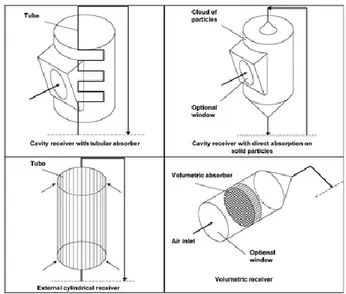
Figure 1.32: Receiver Type ... 47
Figure 1.33: Cavity aperture on CESA-1 Tower on “Plataforma Solar de Almeria” ... 48
Figure 1.34: External Receiver Solar Two ... 49
Figure 1.35: SOLHYCO receiver ... 51
Figure 1.36: SOLUGAS receiver ... 52
Figure 1.37: Left, absorbing and transferring heat for tubular receiver, right absorbing and transferring heat for volumetric receiver ... 53
Figure 1.38: Module of a REFOS volumetric receiver ... 53
Figure 1.39: Cross Section receiver DIAPR ... 54
Figure 1.40: Volumetric receiver and second concentrator on “Plataforma solar de Almeria” ... 54
Figure 1.41: SOLGATE Receiver ... 55
Figure 1.42: SOLTREC Receiver and its integration ... 56
Figure 1.43: Solar particle receiver system ... 57
Figure 1.43: T-S diagram of the Rankine cycle with reheat ... 58
Figure 1.44: Stirling Cycle P-V Diagram ... 59
Figure 1.45: CSIRO Solar Air Turbine Project ... 60
Figure 1.46: Aora Solar Plant on “Plataforma Solar de Almeria” ... 62
Figure 1.47: 247Solar plant[118] ... 62
Figure 1.48: THEMIS Solar System ... 63
Figure 1.49: SOLUGAS plant ... 64
Figure 2.1: Plant scheme ... 66
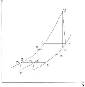
Figure 2.2: T-s diagram of regenerated Joule-Brayton cycle ... 74
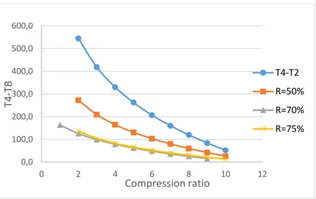
Figure 2.3: Efficiency vs compression ratio ... 76
Figure 2.4: Trend of the temperature difference between the outel gas and compressed air, at different degrees of regeneration ... 77
Figure 2.5: T-s diagram effect of mass flow adjustment ... 77
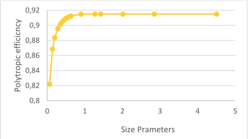
Figure 2.6: Size parameter vs power rate for first and second compressor stage ... 82
Figure 2.7: SP vs polytropic efficiency for first compressor stage ... 82
Figure 2.8: SP vs polytropic efficiency for second compressor stage... 83
Figure 2.9: Size parameter vs power rate for the turbine ... 83
Figure 2.11: Collectors/ Gas turbine efficiency vs Temperature ... 85
Figure 2.12: Overall cycle efficiency vs maximum operative temperature ... 86
Figure 3.1: DNI map on “Sun belt”. ... 87
Figure 3.2: Variation in field layout for latitude 0 °, 20 ° and 60 ° ... 89
Figure 3.3: CDF of DNI (TMY 3) for Seville elaborated by thermodynamic group of University of Seville (source SAM) ... 90
Figure 3.4: Solar multiple trend vs LCoE ... 90
Figure 3.5: Thermoflex operative flowchart ... 91
Figure 3.6: WinDelsol flowchart... 93
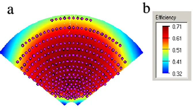
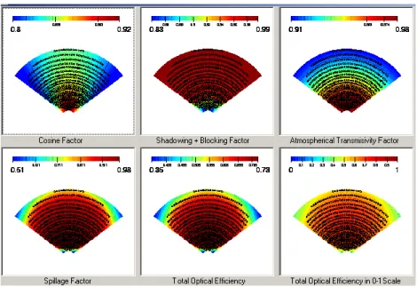
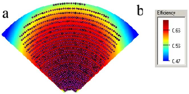
Figure 3.7: 5MW power plant, a) solar field layout with efficiency scale, b) scale values ... 97
Figure 3.8: Factors losses solar fields’ layout of 5 MW power plant ... 97
Figure 3.9: a) front view of receiver b) lateral view of receiver for 5 MW solar field... 98
Figure 3.10:Flux incident receiver on receiver surface in 3D for 5 MW power plant ... 98
Figure 3.11: 10 MW power plant, a) solar field layout with efficiency scale, b) scale values ... 98
Figure 3.12: Factors losses solar fields layout of 10 MW power plant ... 99
Figure 3.13: a) front view of receiver b) lateral view of receiver for 10 MW solar field... 99
Figure 3.14: Flux incident receiver on receiver surface in 3D for 10 MW power plant ... 100
Figure 3.15: 20 MW power plant, a) solar field layout with efficiency scale, b) scale values ... 100
Figure 3.16: Factors losses solar fields layout of 20 MW power plant ... 101
Figure 3.17: a) front view of receiver b) lateral view of receiver for 20 MW solar field... 101
Figure 3.18: Flux incident receiver on receiver surface in 3D for 20 MW power plant ... 102
Figure 3.19: 50 MW power plant, a) solar field layout with efficiency scale, b) scale values ... 102
Figure 3.20: Factors losses solar fields layout of 50 MW power plant ... 103
Figure 3.21: a) front view of receiver b) lateral view of receiver for 50 MW solar field... 103
Figure 3.22: Flux incident receiver on receiver surface in 3D for 50 MW power plant ... 103
Figure 3.24: Power and efficiency vs hour of the day considered ... 111
Figure 3.25: DNI trend vs hour of the day considered ... 111
Figure 3.26: Comparison of energy production between open and closed cycle for each size power plant. ... 112
Figure 4.1: Heliostat field layout of SM=1.2 plant. ... 115
Figure 4.2: Factors losses solar fields’ layout of SM 1.2 ... 115
Figure 4.3: Receiver flux map of SM=1.2 configuration ... 116
Figure 4.4: Receiver view and dimensions; a) front, b) lateral, c) plant of SM = 1.2 configuration. ... 116
Figure 4.5: Heliostat field layout of plant with SM=1.1 ... 117
Figure 4.6: Factors losses solar fields’ layout of SM 1.1 ... 117
Figure 4.7: Receiver view and dimensions; a) front, b) lateral, c) plant of SM = 1.1 configuration. ... 118
Figure 4.8: Receiver flux map of SM=1.1 configuration ... 118
Figure 4.9: Heliostat field layout of plant with SM=1.0 ... 118
Figure 4.10: Factors losses solar fields’ layout of SM 1.0 ... 119
Figure 4.11: Receiver flux map of SM=1.0 configuration ... 119
Figure 4.12: Heliostats field area percentage defocusing vs. hours of considered day ... 122
Figure 4.13: Heliostats field area percentage defocusing vs. DNI ... 122
Figure 4.14: Base pressure of the cycle vs hours of the considered day ... 123
Figure 4.15: Base pressure of the cycle vs DNI ... 123
Figure 4.16: Energy production vs hours of 21st june ... 124
Figure 4.17: Energy production during June 21, March 21, December 22, SM 1.2 ... 125
Figure 4.18: Energy production during June 21, March 21, December 22 ... 126
Figure 4.19: Defocusing percentage of the heliostats field ... 127
Figure 4.20: Cost structure for SM=1.2 configuration ... 134
Figure 4.21: LCoE Trend vs solar multiple ... 139
Figure 5.1: Operation strategy of storage systems ... 142
Figure 5.2: Temperature profile of a HTF inside the tube. ... 145
Figure 5.3: Vapour pressure vs operative temperature for analysed salt [64]. 150 Figure 5.4: Viscosity trend versus temperature of the main salts taken into consideration [64] ... 152
Figure 5.5: Correlation of thermal conductivity according to the average ion weight for different salt families [64] ... 153
Figure 5.6: Plant scheme; 1. Auxiliary compressor, 2. Compressor of GT, 3. Solar tower, 4. Turbine of GT, 5. Cold salt storage tank, 6 Hot salt storage tank,
7 Air-salt heat exchanger, 8 recirculation pump. ... 158
Figure 5.7: Energy produced by thermal energy storage [GWh] ... 161
Figure 5.8: Energy lost vs hours of storage ... 161
Figure 6.1: Micro turbine components Turbec T100 PH ... 168
Figure 6.2: Construction scheme of Turbec T100 ... 168
Figure 6.3: Ansalo Turbec T 100 entire view*0F ... 169
Figure 6.4: Radial inflow turbine of Turbec T 100* ... 169
Figure 6.5: Centrifugal compressor of Turbec T 100* ... 169
Figure 6.6: Geometric dimensions of heliostat ... 172
Figure 6.7: Solar field SM 1 Type 3 heliostats ... 177
Figure 6.8: Solar field SM 1.1 Type 3 heliostats ... 177
Figure 6.9: Solar field SM 1.2 Type 3 heliostats ... 178
Figure 6.10: Solar field SM 1.3 Type 3 heliostats ... 178
Figure 6.11: Incident flux on the receiver for SM 1 and heliostat type 3 ... 179
Figure 6.12: Incident flux on the receiver for SM 1.1 and heliostat type 3 ... 179
Figure 6.13: Incident flux on the receiver for SM 1.2 and heliostat type 3 ... 180
Figure 6.14: Incident flux on the receiver for SM 1.3 and heliostat type 3 ... 180
Figure 6.15: Aiming point of the heliostats for SM 1, SM 1.1, SM 1.2, SM 1.3 and heliostats type 3 ... 181
Figure 6.16: Solar field SM 1 Type 2 heliostats ... 183
Figure 6.17: Solar field SM 1.1 Type 2 heliostats ... 183
Figure 6.18: Solar field SM 1.2 Type 2 heliostats ... 183
Figure 6.19: Solar field SM 1.3 Type 2 heliostats ... 184
Figure 6.20: Incident flux on the receiver for SM 1and heliostat type 2. ... 184
Figure 6.21: Incident flux on the receiver for SM 1.1 and heliostat type 2. ... 184
Figure 6.22: Incident flux on the receiver for SM 1.2 and heliostat type 2. ... 185
Figure 6.23: Incident flux on the receiver for SM 1.3 and heliostat type 2. ... 185
Figure 6.24: Solar field SM 1 Type 3 heliostats ... 187
Figure 6.25: Solar field SM 1.1 Type 3 heliostats ... 187
Figure 6.26: Solar field SM 1.2 Type 3 heliostats ... 187
Figure 6.27: Solar field SM 1.3 Type 3 heliostats ... 188
Figure 6.28: Incident flux on the receiver for SM 1 and heliostat type 3. ... 188
Figure 6.29: Incident flux on the receiver for SM 1.1 and heliostat type 3. ... 188
Figure 6.30: Incident flux on the receiver for SM 1.2 and heliostat type 3. ... 189
Figure 6.31: Incident flux on the receiver for SM 1.3 and heliostat type 3. ... 189
Figure 6.33: Heliostat field efficiency of the three size. ... 190
Figure 6.34: Interception effect of the heliostats type for the SM configuration analysed. ... 191
Figure 6.35: Annual efficiency for all configuration ... 191
Figure 6.36: Referring TS regenerating Joule- Brayton cycle ... 200
Figure 6.37: DNI trend of the 21st June (GTER Seville) ... 202
Figure 6.38: Azimuth trend of the 21st June (GTER Seville) ... 202
Figure 6.39: Zenith trend of the 21st June (GTER Seville) ... 202
Figure 6.40: Heliostats filed efficiency for three heliostats type and SM 1 ... 203
Figure 6.41: Heliostats filed efficiency of heliostats type 3 for the four SM ... 204
Figure 6.42: Zoom in of fig 6.40 of the hours middle day of the trend efficiency. ... 204
Figure 6.43: Incident power on the receiver for SM 1.3 ... 205
Figure 6.44: Incident power on the receiver of heliostats type 3 ... 205
Figure 6.45: Incident flux on the receiver of heliostats type 3... 206
Figure 6.46: Incident flux on the receiver of heliostats type 1... 206
Figure 6.47: Receiver mass flow results of heliostats type 2 ... 207
Figure 6.48: Receiver pressure results of heliostats type 2 ... 207
Figure 6.49: Power to HTF results of heliostats type 2... 208
Figure 6.50: Temperature inlet turbine trend SM 1 ... 208
Figure 6.51: Temperature inlet turbine trend heliostats type 3 ... 209
Figure 6.52: Thermal losses trend SM 1 ... 209
Figure 6.53: Heliostat defocused trend heliostats type 3 ... 210
Figure 6.54: Heliostat defocused trend heliostats type 1 ... 210
Figure 6.55: Power production heliostats types SM 1.3. ... 211
Figure 6.56: Power production heliostats type 3. ... 211
List of table
Table 1.1.1: Specification of some heliostats ,built in the past ... 42
Table 1.2: Air receivers currently developed [100], [101], [33],[102], [36], [103] 50 Table 3.1: Main data input on WinDelsol ... 94
Table 3.2: Receiver first step size and radiative losses. ... 96
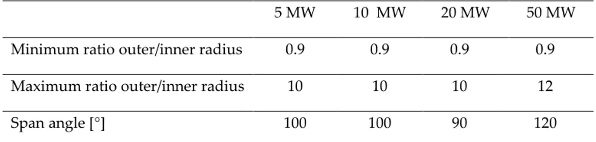
Table 3.3: Input data in WinDelsol for field dimensions. Radii are expressed in terms of tower heights. ... 96
Table 3.4: Matrix of efficiencies of the 5 MW solar field ... 104
Table 3.5: Matrix of efficiencies of the 10 MW solar field ... 104
Table 3.6: Matrix of efficiencies of the 20 MW solar field ... 104
Table 3.7: Matrix of efficiencies of the 50 MW solar field ... 105
Table 3.8: Main data evaluated for first and second stage ... 107
Table 3.9: Main data evaluated for turbine ... 107
Table 3.10: Main Gas turbines regenerators data ... 107
Table 3.11: Main Gas turbines intercoolers data ... 108
Table 3.12: Main low temperature heat exchangers data ... 108
Table 3.13: Main data of open cycle compressors ... 110
Table 3.3.14: Main data of open cycle turbine ... 110
Table 3.15: Closed cycle size parametric analysis results ... 110
Table 3.16: Open cycle size parametric analysis results. ... 111
Table 3.17: Energy comsuption by the auxiliary compressos for closed 50 MW power plant ... 112
Table 4.1: Solar field ratio dimensions and span angle... 115
Table 4.2: Average, maximum and minimum value of each field efficiency of SM 1.2 ... 116
Table 4.3: Average, maximum and minimum value of each field efficiency of SM 1.1 ... 117
Table 4.4:Average, maximum and minimum value of each field efficiency of SM1.0 ... 119
Table 4.5: Matrix of efficiencies SM=1.2 solar field ... 120
Table 4.6: Matrix of efficiencies SM=1.1 solar field ... 120
Table 4.7: Matrix of efficiencies SM=1.0 solar field ... 120
Table 4.8:Mass flow-working hours for June 21, March 21 and December 22 126 Table 4.9: Direct and indirect cost items ... 132
Table 4.10: Cost analysis Thermoflex results... 133
Table 4.11: Cost structure vs solar multiple ... 134
Table 4.13:Monthly energy production (GWh) ... 136
Table 4.14:CF, SF-CF and equivalent hours ... 136
Table 4.15:Monthly working hours ... 136
Table 4.16: Montly mass flow control system working hours ... 137
Table 4.17: Financial data of economic return factor ... 138
Table 4.18: Investment cost used il LCoE analysis ... 138
Table 5.1: W/Q ratio for different HTF (T=250°C, P=100 bar) [64] ... 147
Table 5.2: Solidification temperature for analysed molten salts [64] ... 149
Table 5.3: Boiling and solidification temperature, vapour pressure at 900 ° C for analysed salts [64] ... 150
Table 5.4: Density equation for selected molten salt[57] ... 151
Table 5.5: Molar composition and specific heat for the main salts taken into consideration [57] ... 152
Table 5.6:: Thermal conductivity at the corresponding temperature of the various salts taken into account [64] ... 154
Table 5.7: Figure of merits of the main castings taken into account [57] ... 155
Table 5.8: Specific cost of the salts taken into account ... 156
Table 5.9: Summary of physical and chemical properties for the molten salt analyzed... 157
Table 5.10: Storage system result ... 160
Table 5.11: Optimization solar field results ... 160
Table 5.12: Yearly energy production [GWh] function of solar multiple configuration and hours of storage ... 160
Table 5.13: Units costs of plants ... 162
Table 5.14: Molten salt total costs... 162
Table 5.15: Direct costs [MUSD] of cost analysis ... 163
Table 5.16: Indirect costs [MUSD] of cost analysis ... 163
Table 5.17: Investment costs [MUSD] of cost analysis ... 164
Table 5.18: Levelized Cost of Energy [USD/kWh] ... 164
Table 5.19: Unit Cost of the plants configurations [kUSD/kW] ... 164
Table 6.1: Main MGT manufactures and engine data ... 167
Table 6.2: Heliostat field power results ... 171
Table 6.3: Characteristic data of heliostats ... 174
Table 6.4: Type 3 heliostats field data ... 176
Table 6.5: Performance results of the solar fields for heliostats type 3 ... 181
Table 6.6: Type 2 heliostats field data ... 182
Table 6.7: Performance results of the solar fields for heliostats type 2 ... 185
Table 6.9: Performance results of the solar fields for heliostats type 3 ... 189
Table 6.10: Annual energy production [MWh] ... 212
Table 6.11: Utilization factor [MWh] ... 213
1
Sommario
Oggigiorno, la domanda di energia primaria è aumentata, raggiungendo un incremento del 62.5% rispetto a 20 anni fa. La necessità di risorse rinnovabili ha spinto le politiche governative di tutto il mondo a incoraggiare lo sviluppo di nuovi sistemi di produzione di energia. Fra questi vi sono i sistemi a concentrazione solare (CSPs), una tecnologia che concentra la radiazione solare rendendola disponibile, attraverso un fluido termovettore (HTF) come fonte di calore in un ciclo termodinamico di potenza. Il ciclo di potenza più efficiente, come noto, è quello Joule-Brayton, che in configurazione chiusa consente l'utilizzo di HTF diversi; inoltre, è possibile lavorare in condizioni di pressione elevate, con alta temperatura operativa ed efficienza di conversione. L’uso dell’aria come fluido di lavoro rende di facile gestione il sistema senza rischi. Inoltre unendo il ciclo chiuso con un sistema CSP, il sistema è totalmente privo di combustione e non essendo necessario l’uso di combustibile, non sono emessi inquinanti. Fra i sistemi CSP, la tecnologia a torre è in grado di poter raggiungere più alte temperature, disponibile quindi nel ciclo Brayton, e per questo motivo è stato considerato il suo uso nelle analisi. La risorsa imprevedibile, rappresentata dalla radiazione solare, richiede un metodo di regolazione per il controllo della potenza generata dall’impianto. In questo lavoro, quindi, è stata analizzata la fattibilità di un ciclo Joule-Brayton chiuso senza combustione, in un impianto solare a concentrazione a torre che utilizza un sistema di controllo della portata massica. Nel ciclo è operato un controllo della temperatura di ingresso della turbina della turbina a gas, quando varia la radiazione normale diretta (DNI) attraverso la regolazione della densità del fluido di lavoro; questa regolazione è attuata attraverso una variazione di pressione di base del ciclo. In questo sistema la turbina gas non cambia la portata volumetrica come anche i triangoli di velocità o i rapporti di pressione, quindi variando la densità del fluido di lavoro, attraverso una variazione di pressione, è possibile regolare la portata massica al fine di controllare la TIT. Controllando la TIT, quindi, è possibile controllare la potenza elettrica prodotta dalla turbina a gas sotto diversi carichi termici del DNI. In questo lavoro, diverse configurazioni, in termini di potenza delle macchine, come anche l’utilizzo di accumulo termico (TES) sono stati analizzate, ponendo particolare attenzione alla progettazione
2
del campo eliostati. I risultati mostrano che l’efficienza globale del ciclo, rimane costante sotto differenti carichi termici dovuti alla radiazione solare, indipendentemente dalla potenza della turbina a gas; l’utilizzo di accumulo permette di aumentare le ore di utilizzo dell’impianto come anche il fattore di utilizzazione (UF). L’analisi economica, effettuata attraverso il metodo del Levelised Cost of Electricity (LCoE) ha reso possibile ottenere un valore del multiplo solare (SM) differente rispetto ai valori tipici usati. In fine è stata considerata l’applicazione in micro scala di questo tipo di impianto, al fine di confrontarlo con un sistema commerciale esistente.
3
Abstract
Nowadays, the primary energy demand has increased, rising up to 62.5% compared to 20 years ago. The necessity of the renewable sources has prompted the government policies, around the world, to encourage the development of new energy production systems. One of this is the Concentrating Solar Power system (CSPs), a technology that concentrates the solar radiation making it available, through a heat transfer fluid (HTF), as a heat source in a power thermodynamic cycle. The most efficient power cycle, as we know is the Joule-Brayton one, that in a closed configuration allows to use different HTF; in addition, it is possible to work under pressurized conditions, with high operating temperatures and overall cycle efficiencies. The use of the air, as HTF, makes it easy to manage the system under pressure without risk. Moreover coupling the closed cycle, with CSPs, the system is safely unfired, and no fuel is needed as heat source, therefore no pollutants are produced. In CSPs, the solar tower system is able to gain high temperature, available for the Brayton cycle, so this technology has been taken into account in these analysis. The unplanned source represented by the solar radiation, requires an adjustment method able to control the power production by the plant. In this work it has been analysed a feasibility of an unfired closed Joule-Brayton cycle, in a concentrating solar tower plant, employing a mass flow control system. In the cycle, in order to control the turbine inlet temperature (TIT) of the gas turbine, under Direct Normal Radiation (DNI) variation, a working fluid density adjustment is adopted; this regulation is performed by a base pressure adjustment. In this system, the gas turbine engine, does not change neither the volumetric flow rate nor the speed triangles and the pressure ratios, therefore varying the density of the working fluid, through a pressure variation, the mass flow rate it is adjusted in order to control the TIT. By controlling the TIT, by a mass flow variation, it is possible to control the electrical power produced by the gas turbine under different thermal loads of DNI. In this work, several configurations have been analysed, in term of engines power rate as well as the thermal energy storage (TES) employing, paying particular attention on the heliostats field design. The results show that, the overall cycle efficiency remains constant under different solar radiation loads, independently of the gas turbine power rate; the
4
as well as the utilization factor (UF). The economic analysis, performed by the Levelized Cost of Electricity (LCoE) method, allowed to obtain, a particular value of solar multiple (SM), for the analysed system, respect to the one used up to now . Finally was considered, a case of study of a micro scale application for this kind of plant, in order to compare with a commercial system.
5
Acknowledgements
I would like to thank my research supervisor Prof. Mario Amelio, of the University of Calabria, because he was not only a simply advisor, but a real guide during these past years.
I am also grateful to Prof. Manuel Silva Perez, from the University of Seville, for his valuable comments and suggestions and for giving me the opportunity to meet prominent members of the research world field.
I also want to thank Prof. Vittorio Ferraro and Prof. Michele Scornaienchi for their precious guidance and support.
I would like to thank all my University colleagues as well as the Group of Thermodynamics and Renewable Energy of Seville, for all their help and support.
Least but not last a very special thank you goes to my family, my girlfriend, my friends and all the people that constantly sustained me throughout all these years of hard work.
6
Introduction
Nowadays, the world population raise up with a speed of 1.18% per year; there is a totally annual increasing of about 83 million. The United Nation (UN), during 2015 (Figure 1), estimated the world population growth and established that, keeping constant the growth rate, there will be about 9 billion people by 2030 and 9.7 billion by 2050 [71].
Figure 1: Demographic growth projection [71]
Energy consumptions are directly linked to this increase of population, therefore the requirement of primary energy resources is a perceived problem.
7
A major security requirement of energy supply will be need, particularly in the presence of even much stronger restriction environmental impact laws.
Primary energy consumption refers to the direct use at the source, or supply to users without transformation, of crude energy, that is a type of energy not subjected to any conversion or transformation process. Some example are the exhaustible energy sources (coal, oil, etc.), renewable energy sources (solar, wind, biomass, hydro, geothermal…) and heat energy deriving from the ground of the Earth which allows to produce geothermic energy [72].
The measurement unit commonly used is TEP, (tons of petroleum equivalent, or TOE, tons of oil equivalent). 1 MTEP (106 TEP) is the energy content in one millions tons of oil that is equivalent to a 41.86 × 10¹⁵ Joule.
In last 25 years, from the 1990s up to the 2015, the primary energy demand has increased up to 8000 MTEP to 13000 MTEP, rising up to almost 62.5%.
Also, it is possible to observe from Figure 2, that 85 % of the total energy demand is satisfied by fossil fuels, while only a small part (orange trend) is supplied by renewable sources.
International energy policies, of the last years, promoted and incentivized the reduction of the environmental impact of thermoelectric power plants as well as greenhouse gases, using the development and diffusion of energy product by renewable energy source systems. An energy source is considered renewable, if it can regenerate itself in a short time, compatible with the human life cycle.
From the Kyoto protocol to the lasts European directives “2001/77/CE” / “2009/28/CE”, a common framework for the promotion of energy from renewable sources have been established and mandatory national targets have been set. Regarding the European Union members states these objectives were set on June 30th 2010, the so called “20-20-20”, which, among other goals, made mandatory the renewables contribution (20%) of the total energy consumption in a period of 10 years [73]. These policies have produced, naturally, big changes on electric systems and power grid: the plants performance of renewable system is totally dynamic, mainly because this kind of source is unplanned and random
8
so it is difficult a clear estimation of daily production. For this reason, actually renewable energy does not contribute to the frequency adjustment of the electricity grid. Employing the renewable sources connected to the grid trough the inverter generators, the rotating masses (generally employed in thermoelectric plants) are not used [75].
Renewable energy is an alternative to the traditional fossil fuel and some of it is not introduced pollutant substance, which are usually present in the atmosphere damaging the climate.
The following sources are considered renewable: Solar energy
Wind energy Biomass Sea energy
Hydroelectric source
Solar energy is the most widespread on the Earth because is renewable, available, completely free and largely in excess of the energy demand of the world population. It is necessary to pay attention that, every year, the sun irradiates on the Earth face about 19 billion of MTEP of energy, while the demand, as described before is about 13000 MTEP. The potential energy obtainable from the sun could be a large part of the electric demand.
Nowadays, it is used only a very small part of the huge quantity of energy coming from the sun. In perspective, solar energy will play a significant role, to allow the reversal of the current trend, which is essential for the ecology safe of the planet. The thermal energy arising from solar irradiation can be "intercepted" in many ways and used for various energy needs: for example, thermal energy could be useful for the production of hot water for primary necessities, instead of employing the solar thermal systems for the production of electricity [76].
There are three kinds of technology that allow to use the solar sources: Photovoltaic systems (PVs)
9 Solar thermal systems (STs)
Solar thermodynamics systems (CSPs)
Solar thermal technology is employed to produce heat (for primary necessity), while photovoltaic systems, as known, are suitable to generate electric energy.
Photovoltaics systems, convert directly global normal irradiance, incident on the panel surface, in electricity by employing semiconductor cells (Siliceous) trading on the photovoltaic effect.
Solar thermodynamics, called Concentrating Solar Power (CSP) systems, operates intercepting the direct normal radiation (DNI) by a concentrator, in a receiver, increasing the enthalpy of a heat transfer fluid. This energy is suitable for a power unit to produce electric energy or heat source.
CSP technology, started to be commercialized during the 1980’s, after the first oil crisis, but the decreasing of oil cost and the development of photovoltaics plants declare a temporary downfall of this technology. One of the CSPs disadvantages is the “specific location” compared to the photovoltaics one; practically concentrating systems could gain good plant efficiency only through sites with high solar insolation [78]. These areas, particular adequate for this technology, are usually called “sun belt”, shown in figure 3.
10
However, CSP technology has some advantages compared to the photovoltaic (PV) one [79]:
It is possible to obtain a net conversion efficiency higher than the PVs; Possibility of storage, by the Thermal Energy Storage (TES) employing
molten salt (or other heat transfer fluid) cheaper than the electrochemical storage systems used in the PVs;
Looking at this topic and considering the energy problems examined, the objective of this thesis is to demonstrate the feasibility of a closed Joule-Brayton cycle, in a Concentrating Solar Tower system (CSTs) as a heat source. It has been demonstrated that it is possible the use of air, as heat transfer fluid, without the use of fuel (so unfired). In the cycle is performed a mass flow adjustment, in order to control the Turbine Inlet Temperature (TIT). As will be explained, in this way the electrical power production will be controlled as well.
Firstly it has been used the Joule-Brayton cycle due to the fact that it has the highest the gas turbine yield of the cycle. Secondly, the Brayton cycle is useful in concentrating solar system, and in addition, the closed configuration allows to employing air as heat transfer fluid, working with high temperature obtaining excellent overall cycle efficiency.
The solar tower system, is the only CSP technology that makes it possible to gain high temperature, respect to other technologies, for this reason this kind of plant, has been taken into account in the analysis.
The exploration of the air as HTF, has been conducted because it is a totally free fluid, not polluting, and mainly, working under pressure condition, is not dangerous.
The unplanned source represented by the solar radiation, requires an adjustment method able to control the electrical power produced by the plant.
The core of this work is the mass flow control systems, employed in the cycle, to control the Turbine Inlet Temperature of the gas turbine under different solar radiations load.
In this kind of cycle, the volumetric flow rate, as well as the pressure ratio and the speed triangle of the gas turbine, do not vary; changing the base
11
pressure of the cycle, along with the average density of the working fluid, it is to obtain a mass flow variation.
Keeping fixed the main temperatures and pressures of the cycle, controlling the TIT it is possible to control the electrical power produced.
Different power rates, have been analysed, in different configuration (regarding the use of storage or solar multiple) to optimize the cycle and all component used in the system.
Particularly attention, will be focused on the design of solar field, because it represents the only heat source in the cycle and the major cost voice of the plant. In chapter 1 it will be described the history of concentrating solar systems, the state of the art of the operational and R&D solar tower with gas turbine plants.
Chapter 2 will be dedicated to the model description of the mass flow control system studied in this work, and its parameters as well as the cycle optimization.
In chapter 3 there will be performed an analysis for different power rate sizes, at MW scale, of the gas turbine and of the heliostat field, along with the comparison with an open simple cycle.
In chapter 4 it will be considered the design of the heliostats field for the plant that has employed the control systems.
In chapter 5 a case of study using storage will be analysed; particular attention will be focused on the use of an innovative molten salt, cheaper and more suitable for the high temperature storage.
Chapter 6 will treats the simulation of the control systems and its advantages, in a modified micro gas turbine of a peak power of 500 kW.
Finally it will be presented, the conclusions of these analysis and the outlook for this kind of technology.
12
1.
Chapter 1
Concentrating solar power (CSPs) system
1.1. Solar concentrating fundamentals
Solar radiation is an energy source at high temperature, with an available irradiance, near the sun, about of 65 MW/m2. However only a very small part of this flux, about 1 kW/m2, irradiates the Earth and is available, owing to the huge distance (149.600.000 km) between the Sun and our planet. It is possible to use this “low density” energy, employing optic concentrating systems.
Adding an optic device between the radiation source and the absorbent surface (receiver), it is possible to concentrate this radiation on a smaller surface, increasing the density and achieving both higher thermal flux and lower thermal loss. This mechanism allows to achieve high temperature on the receiver surface (absorber), and then increasing the conversion efficiency from heat to mechanical work.
Figure 1.1 : Schematic solar concentrating fundamentals
In figure 1.1 it is possible to observe the operating fundamentals of concentrating technology; flux E across the A section and exit from A’ < A.
Assuming that there are no losses inside the concentrating system, we can write the following conservation law:
13
𝐸 ∙ 𝐴 = 𝐸
′∙ 𝐴′
(1.1)
The geometric concentrating ratio, so, has been defined as:
𝐶 =
𝐴𝐴′
(1.2)
This ratio has an upper limit depending of the kind of concentrating system, which could have two configurations:
Three-dimensional (point-focus); Bi-dimensional (line-focus).
The upper limit for three- dimensional system, could be described following the Rabl methodology [1]
Figure 1.2: Schematic solar concentrating fundamentals
The Sun (S) and the absorbent surface (Aabs) were considered as black bodies. The Sun could be assumed as isotropic sphere having radius r and a distance from the Earth R. The temperatures assumed for the Sun and absorbent surface are respectively Ts and Tsa. The black body is defined as an ideal body or surface that completely absorbs all radiant energy incident upon it, with no reflection and that radiates at all frequencies with a spectral energy distribution dependent on its absolute temperature. Then, it is possible to write:
14
𝜏 = 𝜌 = 0
(1.4)
Referring to figure 1.2 and considering an ideal concentrating system, the incident irradiance on absorbent surface is proportional to the radiation intercepted by the aperture A. This effect is expressed by the equation:
𝑄
𝑟𝑎𝑑= 4𝜋𝑟
2𝜎𝑇
𝑠4(1.5)
Where σ is the Stefan-Boltzmann constant. The view factor is defined below F S-A:
𝐹
𝑆−𝐴=
𝐴4𝜋𝑅2
(1.6)
Replacing the equation (1.6) in (1.5) we obtain:
𝑄
𝑟𝑎𝑑,𝑆−𝐴= 𝐹
𝑆−𝐴∙ 𝑄
𝑟𝑎𝑑= 𝐴
𝑟2 𝑅2𝜎𝑇
𝑠4
(1.7)
Following the same methodology for the receiver (absorbed) surface:
𝑄
𝑟𝑎𝑑,𝑎𝑠= 𝐴
𝑎𝑠𝜎𝑇
𝑎𝑠4(1.8)
Also defining for this case, the view factor𝐹𝐴𝑎𝑠−𝑆< 1, and replacing in (1.8) we
obtain:
𝑄
𝑟𝑎𝑑,𝐴𝑎𝑠−𝑆= 𝐹
𝐴𝑎𝑠−𝑆∙ 𝑄
𝑟𝑎𝑑𝑎𝑠= 𝐴
𝑎𝑠𝐹
𝐴𝑎𝑠−𝑆𝜎𝑇
𝑎𝑠4
(1.9)
Under steady state conditions, both bodies havet the same temperature T; it is possible to write the following equality between flows:
𝑄
𝑟𝑎𝑑,𝑆−𝐴= 𝑄
𝑟𝑎𝑑,𝐴𝑎𝑠−𝑆(1.10)
Replacing (1.7) and (1.9) in (1.10) equation, we obtain:
𝐴
𝑟2𝑅2
𝜎𝑇
4
= 𝐴
𝑎𝑠
𝐹
𝐴𝑎𝑠−𝑆𝜎𝑇
𝑎𝑠4
(1.11)
From this last equation, the concentration ratio is obtained:
𝐶 =
𝐴 𝐴𝑎𝑠=
𝑅2 𝑟2∙ 𝐹
𝐴𝑎𝑠−𝑆= 𝐹
𝐴𝑎𝑠−𝑆∙
1 𝑠𝑒𝑛2𝜃(1.12)
Analysing the (1.12) it is obvious that the following inequality will always be valid:
15
If the absorbent surface is added in a transparent medium, of refractive index n, the incident radiation is enclosed in the range ± θ with θ ≤ θn.
According to the Snell law, when the medium changes, the following equation keeps constant:
𝑠𝑒𝑛 𝜃𝑐
𝑠𝑒𝑛 𝜃𝑛
=
𝑛
𝑛𝑐
(1.14)
Where:
𝜃𝑐 is the incidence angle; 𝜃𝑛 is the refraction angle;
Assuming, hypothetically, nc=1 we have:
𝑠𝑒𝑛𝜃
𝑛=
1
𝑛
𝑠𝑒𝑛𝜃
𝑐(1.15)
The half-opening θc angle for the Sun-Earth system is 4.653 mrad. Consequently, for a three-dimensional concentration system, the ratio of maximum concentration is:
𝐶
3𝐷≤ (
1𝑠𝑒𝑛2𝜃
𝑐
) ≈ 46225 (1.16)
This limit can be reached with an ideal three-dimensional concentrator. For a two-dimensional concentration system, we have:
𝐶
2𝐷≤ (
1𝑠𝑒𝑛2𝜃
𝑐
) ≈ 215
(1.17)
The obtained value (C2D) is significantly lower than the three-dimensional one (C3D), so a higher temperature of heat transfer fluid (in general) could be reached in solar tower, compared to the parabolic trough collector. This topic will be in depth explained in the following sessions.
The available power, upstream of the concentration system, can be obtained with the equation (1.18), however only a part of this power will be transferred to the receiver.
The relation between these two powers determines the optical efficiency of the concentration system:
16
𝑄̇
𝑑𝑖𝑠𝑝= ∫ 𝐼
𝑆 𝑏,𝑛𝑑𝑆
(1.18)
𝜂
𝑜𝑝𝑡=
𝑄̇𝑟𝑒𝑐𝑄̇𝑑𝑖𝑠𝑝
(1.19)
The receiver has been designed to absorb the maximum power from the solar radiation concentrated on it; an ideal receiver, in fact, it has a thermal behaviour like a black body and the only loss is for radiative emission.
In real applications, the same situation does not occur because there are other losses: an example are the convention losses. When the solar rays are concentrated on the receiver surface, its temperature begins to increase together with the loss mechanisms.
This process is time-variant until the stationarity conditions are not achieved: at this point, the input power, coming from the concentration system, matches the sum of the power transferred to the heat transfer fluid while it takes from the thermal and optical losses. A part of the input thermal power is absorbed by the surface; the other part is reflected and transmitted according to the optical properties of the absorber surface.
The power transferred to the heat transfer fluid is:
𝑄̇
𝑎𝑏𝑠= 𝑚̇
𝐻𝑇𝐹(ℎ
𝑜𝑢𝑡− ℎ
𝑖𝑛)
(1.20)
Where:
𝑚̇𝐻𝑇𝐹 is heat transfer fluid mass flow rate (kg/sec)
(ℎ𝑜𝑢𝑡− ℎ𝑖𝑛) is the enthalpy variation from inlet and outlet of the receiver
(J/kg)
Total inlet thermal power includes the absorbed power and the losses:
𝑄̇
𝑖𝑛= 𝑄̇
𝑎𝑏𝑠+ 𝑄̇
𝑙𝑜𝑠𝑠(1.21)
Explicate the 𝑄̇𝑙𝑜𝑠𝑠 we obtain:
𝑄̇
𝑙𝑜𝑠𝑠= 𝑄̇
𝑟𝑎𝑑+𝑄
̇
𝑐𝑜𝑛𝑣+ 𝑄̇
𝑐𝑜𝑛𝑑+ 𝑄̇
𝑟𝑖𝑓𝑙(1.22)
From all these losses explained in (1.22), the most significant is the radiation loss: the surface of the receiver emits thermal power proportional to the fourth
17
power of the temperature; it is clear that this is a phenomenon which dispels a lot of energy. In order to simplify the discussion, constant receiver surface temperature is assumed; the power lost by radiation is equal to:
𝑄̇
𝑟𝑎𝑑= 𝜀𝜎𝐴
𝑟𝑒𝑐𝐹
𝑟−𝑒𝑥(𝑇
𝑟𝑒𝑐4− 𝑇
𝑒𝑥4)
(1.23)
Where:
𝐴𝑟𝑒𝑐 is the scatter receiver surface [m2];
Trec is the scatter homogenous surface receiver temperature [K];
Tex is the ambient temperature [K];
Fr-ex is the view geometric factor receiver-external ambient.
The air motion around the receiver causes convection losses; in almost all of them CSP plants are the sum of two contributions: forced convection caused by wind and natural convection are caused by local temperature gradients. It is difficult to evaluate these losses, because very often there are influenced by the radiation and vice versa.
There are numerical methods that, albeit with great approximation, allow to separate the two contributions [2]. A general expression for this kind of loss is:
𝑄 = ℎ𝐴
𝑟𝑒𝑐(𝑇
𝑟𝑒𝑐− 𝑇
𝑒𝑥)
(1.24)
Where:
h is average heat transfer convective coefficient (W/m2K)
There is reflection loss because the receiver is not a (perfect) black body and, therefore, it cannot absorb all of the incident radiations. One part is absorbed and the other is reflected:
𝑄̇
𝑟𝑒𝑓𝑙= (1 − 𝛼)𝐴
𝑟𝑒𝑐𝐶𝐼
𝑏,𝑛(1.25)
Finally, the conduction losses (one-dimensional) can be expressed by (1.26):
𝑄
𝑐𝑜𝑛𝑑= 𝐾
𝑆𝐿
(𝑇
𝑠1− 𝑇
𝑠2)
(1.26)
Where:
K is the thermal conductivity of the material [W/m K]; L is the thickness [m];
18 S is the dispersing surface[m2];
(𝑇𝑠1− 𝑇 𝑠2) is the temperature difference between the two sections [K].
The receiver efficiency can be expressed as:
𝜂
𝑟𝑒𝑐=
𝑄̇𝑖𝑛−𝑄̇𝑙𝑜𝑠𝑠
𝑄̇𝑑𝑖𝑠𝑝
(1.27)
To evaluate the dependence of this efficiency on the surface temperature and the concentration ratio, conduction and reflection losses can be neglected in a first approximation. Combining the relations (1.23), (1.24) and (1.25) we get:
𝜂
𝑟𝑒𝑐= α −
𝜀𝜎(𝑇𝑟𝑒𝑐4 −𝑇𝑒𝑥4)CI𝑏,𝑛
−
ℎ(𝑇𝑟𝑒𝑐−𝑇𝑒𝑥)
CI𝑏,𝑛
(1.28)
Assuming, hypothetically that: 𝜀 = 𝛼 = 0.97
𝑇𝑒𝑥= 298 𝐾 I𝑏,𝑛= 850 𝑊/𝑚2 ℎ = 20 𝑊/𝑚2𝐾
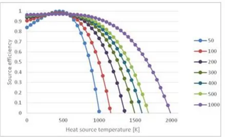
In figure 1.3 it has been shown the trend efficiency as function of the source temperature for different concentration ratio (C).
Figure 1.3: Solar collector efficiency vs source temperature for different concentration ratio.
19
Increasing the temperature, automatically the radiation and convection losses rise as well. When losses match the energy produced, the net useful energy is nil and the receiver achieves its maximum temperature [3]. In practice, the coefficients α and ε cannot be considered constant along the entire solar spectrum. It is preferred to achieve a receiver with higher absorption coefficient and lower possible emissivity. Typically, selective coatings compose the absorbing surface, which plays a fundamental role in stabilizing the losses [4].
According to Kirchhoff’s law, in thermal equilibrium (constant temperature), for a particular surface, we have that:
𝜀(𝜆) = 𝛼(𝜆) (1.29)
If the solar spectrum and the radiation spectrum, emitted by the receiver, are sufficiently different from each other, it is possible to use a material whose α is characterized by a strong dependence on the wavelength, to obtain high values of α and low emissivity values ε [5]. This is a proven fact because the solar spectrum is comparable to the one of a black body at a temperature of 5777 K, while a solar receiver can reach temperatures in the range of 1000 ° C during its operation.
The best solution, therefore, is to obtain high values of α in the range of visible light (390 - 700 nm) and, at the same time, to limit the emissivity ε to the range 700nm – 1mm, below the infrared.
20
Figure 1.5: Electromagnetic spectrum and visible radiation range
The reason for which it is necessary to have the highest receiver temperature possible is related to the conversion efficiency: a higher temperature allows to gain a higher conversion efficiency.
Usually the heat produced by concentrating systems, it is converted into mechanical work, by means of conventional generation systems (thermodynamic cycles) and, subsequently, in electricity. It is possible to evaluate the global efficiency of the system, linking the receiver efficiency with the one of an ideal Carnot cycle, operating between the receiver temperatures and the ambient.
Considering the following equation:
𝜂
𝐶𝑎𝑟𝑛𝑜𝑡= 1 −
𝑄𝑜𝑢𝑡
𝑄𝑖𝑛
= 1 −
𝑇𝑒𝑥
𝑇𝑟𝑒𝑐
(1.29)
From the product between the Carnot efficiency, defined by (1.29), and the receiver efficiency, obtained with the (1.28), overall efficiency has been evaluated:
21
Figure 1.6: Carnot efficiency vs temperature
Figure 1.7: Global efficiency vs temperature for different concentration ratio C Observing the trend in figure 1.7 appears that there is an optimum operative temperature for every concentration ratio; this optimum temperature can be calculated by calculating the derivate of the overall efficiency with respect to temperature equal to zero:
𝜕𝜂𝑂𝑣𝑒𝑟𝑎𝑙𝑙
𝜕𝑇
= 0
(1.31)
This temperature will be the optimal temperature for the operation of the solar receiver and it is an important parameter for a CSP plant.
22
1.2. Brief history of the concentrating solar technology
The technology of concentrating solar plants is often traced to the legend of the "burning mirrors" of Archimedes. The development for the purpose of energy production of solar concentration technology was at the began at the last century with prototypes already very similar to the current ones, in shape and concept.
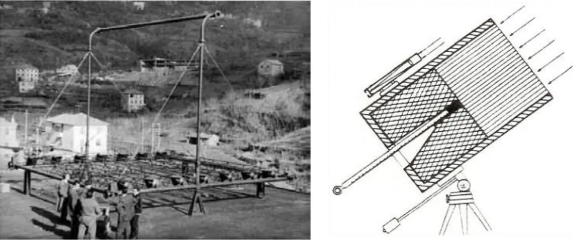
In this regard, it can lead as an example the plant built by Frank Schumann (1862-1918) in Egypt, which was completed in 1912. The system was used for the production of steam, to pump water from the Nile with storage in hot water (Figure 1.8).
Figure 1.8 : Linear Parabolic Solar System (44-51 kW) built by Frank Schumann at Meadi in Egypt in 1912
The real development started, however, in the 60s and 70s in the United States, in France and in Russia, through experiments related to the strength of materials subjected to high radiant flux and high temperatures caused by the solar concentration.
Professor G. Francia in 1964 created a system of mirrors with fixed directional linear collector, which is prior to the current technology of Fresnel mirrors. The absorber were protected by honeycomb cells to decrease the losses due to convection and radiation.
The plant that applied these concepts, built in Marseilles, was able to produce steam that was collected from the top of the collector and was intended to give power to a turbine in order to produce power generation (Figure 1.9).
23
Figure 1.9: Concentrating solar system with linear mirrors and honeycomb absorber for steam production (left), absorber diagram (right).
After these pioneering achievements in the late '70s, the Plataforma Solar de Almeria was created, thanks to an European collaboration, dedicated to research on solar concentration and other environmental applications of solar energy. Following, the first real installations were built in Adrano (Sicily) in 1981; the Eurelios project was the first solar tower system built in the world. the International Energy Agency’s Small Solar Systems
The tower (IEA-SSPS) was built the nor of the national Spanish project Central Electro solar de Almeria-1 (CESA-1). The IEA-SSPS project was the first demonstration project that delivered electricity to the grid in Europe. The combination of the IEA-SSPS and CESA-1 infrastructures in around 1987 was the origin of the Plataforma Solar de Almeria, which has played a pivotal role in the second take-off of CSP technologies worldwide.
Another important project was VastSolar sodium receiver modular technology demonstration plant, in Australia, or of Graphite Solar Power graphite storage tower technology demonstration plant also in Australia.
In the middle of the 80’s also began the construction of parabolic trough plants (United States) and also started the first tests on the Dish-Stirling technology (parabolic dish) [39].
1.3. Concentrating solar technology
A generic CSP (Concentrated Solar Power) plant is characterized by its own main components:
24 Concentration and reflection system; Receiver;
Heat transfer fluid; Storage system;
Conversion system or power unit.
With regard to this last component, the conversion unit choice has been usually made on the economic evaluation and on the use heat-produced: air conditioning, generation of heat for industrial processes and for the production of energy.
Concentration solar plants can be divided into two main groups: line focus and point focus, and are respectively two-dimensional concentration and three- dimensional systems.
As mentioned previously, the first kind has the concentration ratios C = 25-26 and maximum temperatures not more than 550 ° C, the second one however, could have a concentration ratios C> 500 and maximum temperatures of about 1000 ° C.
Nowadays, the market leaders are the parabolic trough system , due to their relative ease construction. Central Receiver Systems (CRSs) are experiencing a very rapid growth period as all efforts to lower their LCOE (Levelized Cost of Energy) are yielding their benefits.
1.3.1. Linear Parabolic Collectors (PTCs)
The concentration system consists of parabolic mirrors which rotate on a single axis. These mirrors reflect and concentrate the direct normal radiation on a receiver tube placed in the optical axis of the cylinder.
25
Figure 1.10: Parabolic linear collectors
They have an average concentration ratio of about 60-100; the heat transfer fluid flows inside the receiver tube, absorbing heat and reaching the desired temperature. A series of heat exchangers (evaporators, super heaters, condensers) located downstream of the solar field, allow the generation of steam, which is then expanded into a turbine.
The structure is made of galvanized steel. The reflector, with the receiver, moves, rotating around an axis, called tracking axis, which follows the Sun in its apparent motion in the sky.
In figure 1.11, it is possible to observe a typical parabolic troughs technology, of 50 MWe size (such as Andasol-1 for example), which uses synthetic oils such as heat transfer fluid and mixtures of molten salts for energy storage.
Figure 1.11: Parabolic troughs collector system
The performance of this type of plant is strongly influenced by the heat fluid transfer. It works with synthetic oils with temperatures above 200 ° C: VP-1, an
26
eutectic mixture consisting of 73.5% of diphenyl oxide and 26.5% of biphenyl is the most used synthetic oil with a maximum temperature of about 395 ° C. The most important factor to consider is the stability of the heat transfer fluid: solidification at about 14 ° C requires the use of auxiliary heating systems; the maximum temperature limit also places a limit on the thermodynamic efficiency of the power cycle. Several research programs have concentrated their work on the study of alternative fluids: molten salts, atmospheric air, water / steam [3].
The DISS project in started 1999 (Direct Solar Steam) at the Almeria Solar Platform in Spain, to facilitate the production of steam and to avoid losses of irreversibility of heat exchange in the exchangers; steam at 100 bar and 400 ° C has been generated directly within the linear receiver. Although this solution seemed very advantageous, there has been a small increase in the efficiency of the plant but great difficulties in dealing with a more complex two-phase fluid and storage systems [6].
Figure 1.12: Direct Solar Steam System Plant
When the energy storage becomes a priority, the best performing fluid so far is a mixture of molten salts: that consists in a mixture composed of 40% of potassium nitrate (KNO3) and 60% sodium nitrate (NaNO3). High availability, low cost, non-flammability, high thermal capacity and temperatures in the range between 260-600 °C make this fluid directly usable both as a heat transfer fluid in the field of linear parabolic collectors as well as a storage medium.
The first company to investigate the operation of PTC plants with molten salts was the “Archimede Solar Energy Company”, that produced a molten salt plant and also used selective coatings, able to withstand the higher temperatures for the molten salts, for the linear receiver. [7]
27
Unfortunately, despite all the benefits that molten salts can offer, their solidification occurs at very high temperatures (238° C) which represents a problem rather important, during cold start-up [8].
Figure 1.13: Pressure Air System Design
Finally, even the used as the heat transfer fluid from the Airlight Energy has realized that linear parabolic collectors pressurized air at 650 ° C. The system schematization is shown in figure 1.13, as possible to observe the reflective surface of which is made with thin polyester film and the accumulation is based on siliceous sand masses.
The receiver of a linear parabolic collector, typically, is a tube made in steel surrounded by another glass tube. Vacuum is applied between the two tubes reducing convection losses [83]. On the steel tube, instead, there are selective coatings to obtain low emissivity (<30% in infrared) and high absorption coefficient (> 90%).
These coatings are used to reduce radiation losses and to increase the performance of the solar field [3]. The parabolic troughs are already the most developed form of technology, covering 80% of the total installed power CSP, with global efficiencies of 14-16% [9], offering modularity, cogeneration and hybridization possibility.
1.3.2. Linear Fresnel Reflectors (LFR)
Fresnel reflectors, shown in figure 1.15, are in essence a series of reflective elements, which are distributed linearly along a surface and constitute a larger reflector. Many files of these reflectors focus on the solar radiation on a linear receiver positioned parallel to the axis of rotation of the reflector. Also on the same receiver, a parabolic collector is installed, in order to optimize the interception of solar radiation.
28
Figure 1.14 : Linear Fresnel reflector system
Figure 1.15 : Linear Fresnel reflector system in “Plataforma Solar de Almeria” In the receiver tube, flows the heat transfer fluid, which usually consists of water. The water mainly used because there is no need of an additionally heat exchanger. Since Fresnel reflectors are the less efficient among the four CSP technologies analysed, adding heat exchanger would worsen even more the overall efficiency. The advantage of this technology is represented by the low cost of realization: each reflective element, in fact, has the same size and can be oriented. This allows the use of mirrors almost flat or slightly curved. Taking advantage of low costs and using in a smart way the land available, one can conceive a simple and inexpensive facility, though not very efficient, with the overall efficiencies not exceeding 12% [9]. Last researches in particular are pushing LFR to a different level which (called Advanced LFR), with higher performance second stage concentrators and new primaries (eaten due matched) to operate at higher temperatures than PTs even, at higher efficiency
29
and lower cost. With these kind of technology is expected to achieve annual plant efficiencies (solar to electricity) of up to 15%, operating directly with molten salts as heat transfer fluid [121].
1.3.3. Parabolic Dish Collectors (PDCs)
The parabolic dish collectors are three-dimensional concentrators; in fact, the solar radiation is focused on a point, using the two axis solar tracking systems. The receiver is located on focal point of the parabolic dish and, usually, the power unit is a Stirling engine, or in some experimental applications, a micro gas turbine.
Figure 1.16: Parabolic dish
The ideal shape of the reflective surface (paraboloid) allows to reach very high concentration ratios (> 1000). The parabolic dish systems reach high temperatures (> 750 ° C) and thermal flows on equally large receivers, and have a conversion efficiency that could reaches about 25-28% [9].
The size of the dish depends on the desired power level and conversion efficiency: a 5-kWe Stirling engine requires a disk of about 5 meters in diameter, while for a 25 kWe plant a 10-meter diameter is sufficient.
The advantages of these systems include modularity, the ability to build standalone systems and the absence of cooling systems. On the other hand, the main disadvantage is the inability to accumulate thermal energy.
30
Parabolic dish systems although are already technologically developed, they have very high maintenance cost due to mechanical failure and thermal fluid leakage [82] (helium and hydrogen in Stirling engines).
From an economic point of view, these systems are not comparable with photovoltaic PV systems, as they also do not allow energy storage (cheap) and have a specific cost of about $ 2000 / kW against the $ 10,000 / kW of PDC systems [10].
1.3.4. Concentrating panel photolytic system(CPV)
CPV systems concentrate the solar beams on the PV (photovoltaic) cells . High performance PV cells are expensive and CPV collectors overcome this drawback. In CPV collectors, concentrated solar beams are reflected on the PV cells which are more cost-effective than stand-alone PV cells.
Therefore, the efficiency of this system would be higher than a common PV cell and this enhancement occurs with lower costs. On the other hand, the number of PV cells would be decreased by using CPV collectors. Also, PVT collector needs to be taken into account to generate both thermal and electrical energy simultaneously.
The back temperature of PV cells would be a waste heat recovery for increasing the performance of these cells by cooling and absorbing the thermal energy for other applications such as space heating or water heating.
CPVT system is a hybrid application of PVT( Photovoltaic Thermal) and CPV collectors for achieving more performance. There are two disadvantages of PVT systems. First, generating desired amount of electrical energy from PV cells needs high investments. Second, the thermal energy of these systems are used for only low-temperature applications.
In a CPVT system, both of these demerits are covered by maintaining the PV cells in a moderated temperature and utilizing the spectrum concentration. In Figure 1.17 it is shown a CPVT system.
31
Figure 1.17: Concentratin Photovoltaic panel
1.3.5. Solar tower systems with central receiver (CRS)
In these systems, a solar field composed by some mirrors, also known as heliostats, collect and concentrate the energy coming from the Sun on the receiver, placed at the top of a tower. The thermal power available to the receiver is then converted into mechanical energy by the power unit.