Subsurface flow and transport modelling at the hillslope scale

(1)

Università degli Studi Roma Tre i

UNIVERSITY OF ROMA TRE

Faculty of Engineering

Doctoral School of Engineering

Civil Engineering Section

PhD in Civil Engineering

XXVI Cycle

Doctoral Thesis

Subsurface Flow and Transport Modelling at the Hillslope

scale

Candidate: Melkamu Alebachew Ali Supervisor : Prof. Aldo Fiori

PhD Coordinator: Prof. Aldo Fiori

Roma,

April 2014

(2)

Università degli Studi Roma Tre ii

Doctoral School of Engineering/PhD in Civil Engineering

_______________________________________________

SCUOLA DOTTORALE / DOTTORATO DI RICERCA IN

XXVI

CICLO DEL CORSO DI DOTTORATO

Subsurface Flow and Transport Modelling at the Hillslope

scale

________________________________________________

Titolo della tesi

Melkamu Ali __________________

Nome e Cognome del dottorando

firma

Prof. Aldo Fiori

__________________

Docente Guida/Tutor: Prof.

firma

Prof. Aldo Fiori

__________________

(3)

Flow and Transport Modelling

Università degli Studi Roma Tre iii

Collana delle tesi di Dottorato di Ricerca In Scienze dell’Ingegneria Civile

Università degli Studi Roma Tre Tesi n° xx

(4)

Università degli Studi Roma Tre iv

Dedicated to: To the memory of my father, Alebachew Ali who passed

away at the end of the completion of this thesis. I miss him every day, but I am glad to know he saw this process through its completion, offering the support to make it possible, as well as lots of encouragement. Thank you father for your friendly advice, your prayer always help me in all the time of my successes.

(5)

Università degli Studi Roma Tre v

Subsurface Flow and Transport Modelling at the Hillslope

scale

Abstract

In hilly and humid forest areas with highly conductive soils, subsurface flow consider as the main mechanism of stream flow generation and responsible for the transport of solutes into the surface water bodies which is transported through the subsurface soil. However, the contribution of the subsurface flow is poorly represented in current generation of land surface hydrological models (LSMs). The lack of physical basis of their common parameterizations precludes a priori estimation, which is a major drawback for prediction in ungauged basins. This thesis is organized in to three sections which analyze the subsurface flow and transport through numerical modeling starting from a simple analysis of homogenous system to complex hillslope with variable soil and topographic properties.

First, the relation Q(S) (where Q is the discharge and S is the saturated storage in the hillslope), as a function of some simple structural parameters is evaluated through two-dimensional numerical simulations and makes use of dimensionless quantities. The method lies in between simple analytical approaches, like those based on the Boussinesq formulation, and more complex distributed models. The results confirm the validity of the widely used power law assumption forQ(S). Similar relations can be obtained by performing a standard recession curve analysis.

(6)

Università degli Studi Roma Tre vi relating to subsurface flow is developed using the Richards’ equation. These parameterizations are derived through a two-step up-scaling procedure: firstly, through simulations with a physically based subsurface flow model for idealized three dimensional rectangular hillslopes, accounting for within-hillslope random heterogeneity of soil hydraulic properties, and then through subsequent up-scaling to the catchment scale by accounting for between-hillslope and within-catchment heterogeneity of topographic features. These theoretical simulation results produced parameterizations of the storage-discharge relationship in terms of soil hydraulic properties, topographic slope and their heterogeneities that were consistent with results of previous studies. The resulted parameterization is regionalized across 50 actual catchments in eastern United States, and compared with the equivalent empirical results obtained on the basis of analysis of observed streamflow recession curves, revealed a systematic inconsistency. It was found that the difference between the theoretical and empirically derived results could be explained, to first order, by climate in the form of climatic aridity index.

Third, the performances of four different models of solute transport in catchments were analysed. The models employ the concept of travel time distribution. A recapitulation and critical analysis of the models and their basic assumptions is performed first, emphasizing their limitations and potential problems arising in their application. Then, detailed numerical experiments are used as a benchmark for the calibration and the assessment of the models’ capabilities to simulate transport. The scope of the exercise is to test the performance of the models and their limitations in the ideal case in which the catchment system and all the hydrological variables (flow, concentration, storage, etc.) are perfectly known at any level of detail. The performance of the models and their limitations is presented and discussed. The results suggest that a time invariant formulation of the travel time distribution is usually inappropriate and not much effective in predicting transport.

(7)

Università degli Studi Roma Tre vii

Acknowledgements

First and above all, I praise the Almighty God for providing me this opportunity and granting me the capability to proceed successfully. This PhD work appears in its current form with the assistance and guidance of several people. I would thereforelike to forward my sincere thanks to all of them.

Foremost, I would like to express my sincere gratitude to my advisor Prof. Aldo Fiori for his continuous support of my PhD study and research, for his patience, motivation, enthusiasm, and immense knowledge. His guidance helped me in all the time of research and writing of this thesis. I could not have imagined having a better advisor and mentor for my PhD study.

Besides my advisor, I would like to thank Prof. Murugesu Sivapalan for the opportunity he has offered me to stay at the University of Illinois Urbana Champaign for one year as exchange scholar and allowing me to be part of his research project. His encouragement, insightful comments, and hard questions help me to improve my understanding in the subject matter.

My sincere thanks also goes to the co-authors of my papers Dr. Giorgio, Dr. Sheng Ye, Dr. Hong-yi Li, Dr.Maoyi Huang and Dr. L. Ruby Leung for their hard-work, willingness to help, and knowledge. Special thanks for Dr. Sheng Ye for her assistance and providing me the necessary data. I should also mention Northwest Pacific Lab for allowing me to visit the laboratory and their assistant and hospitality during my stay.

Thanks also to all professors and the members of the Hydraulic and Hydrology lab at the Civil Engineering Department, University of RomaTre providing me good friendship and support. My friends in Italy and other parts of the World were also sources of laughter, joy, and support. Special thanks goes to Fish, Ephi, Ademe, Tsehaye, Eleni, Feke, Sol and Siraj. I had great time with you and

(8)

Università degli Studi Roma Tre viii am very happy that, in many cases, my friendships with you have extended well beyond our shared time in Rome.

Most importantly, none of this would have been possible without the love and patience of my family. I would like to express my heart-felt gratitude to my family. Thank you for your love, support, and strong belief in me. Without you, I would not be the person I am today. I love them so much.

Above all I would like to thank my lovely wife Rosi, whose love and encouragement allowed me to finish this journey. She is keeping me healthy in all the late nights and early mornings. She already has my heart so my heartfelt thanks go to her and thank you for being my best friend. I owe you everything.

Melkamu Alebachew 2004

(9)

Università degli Studi Roma Tre ix

Subsurface Flow and Transport Modeling at

the Hillslope scale

Melkamu Alebachew Ali

Dissertation for the degree of Doctor of Science in Civil Engineering to be presented with due permission of the Department of Engineering, for public examination and debate at the University of RomaTre

(10)

Università degli Studi Roma Tre x

List of Figures

Figure 2.1: Variability of catchment and hydrological processes at a range of space scale (Blöschl and Sivapalan, 1995) ... 11 Figure 2.2: Schematic view of catchment with its hillslope units and hillslope

discretization scheme (the arrow indicates the flow direction to the streams) ... 13 Figure 2.3μ Darcy’s law experiment ... 15 Figure 2.4: Soil water characteristic curves for selected soils ranges from sand to

clay (Tuller and Or, 2004) ... 18 Figure 2.5: Defination sketch for the Dupuit – Boussinesq aquifer model (

Brutseart and Nieber, 1977) ... 25 Figure 3.1: Illustration sketch of the conceptual model for the hillslope ... 35 Figure 3.2: Water discharge (a) and saturated storage (b) against time for

different soil properties. (Sand, Loamy sand, loam, Silt loam and clay soils) ... 40 Figure 3.3: The relation between dimensionless saturated storage and discharge

from steady state flow simulations. The dots represent the numerical results, while the solid line represents the fitted power-law function. (a) Horizontal slope; (b) 5º slope; (c) 10º (d) 20º (e) 30º and (f) 45º ... 43 Figure 3.4: Approximated relation between the slope of the catchment and the

coefficient b ... 44 Figure 3.5: Comparison of the storage-discharge relation from steady state

simulation with the same obtained by transient simulations. (a) Horizontal slope; (b) 5º slope; (c) 10º slope; (d) 20º slope; (e) 30º slope; (f) 45º slope .... 46 Figure 3.6: Practically, it is hardly possible to measure storage of water in the

subsurface; thus it is more convenient to calculate the storage-discharge indirectly from discharge during no-rain conditions (recession curve analysis). The plot displays -dQ/dt against Q from recession analysis to cross check the possibility of determining the relation curve using the steady state analysis. The rate of discharge dQ/dt is calculated from simple finite difference and Q is also taken as the average value of the consecutive time steps. (a) Horizontal slope; (b) 5_{⁰ slope; (c) 10⁰ slope; (d) 20⁰ slope;} (e) 30_{⁰ slope; (f) 45⁰ slope ... 49} Figure 4.1: Examples of spatial distribution of hydraulic conductivity [lnK] are

shown for mean surface hydraulic conductivity Ks of 28 ms-1_{, topographic}

slope of 10º and f = 1m-1_{with different values of spatial variability} lnk2

(the color legends are shown in lnK where K is in ms-1_{) The flow domain,}

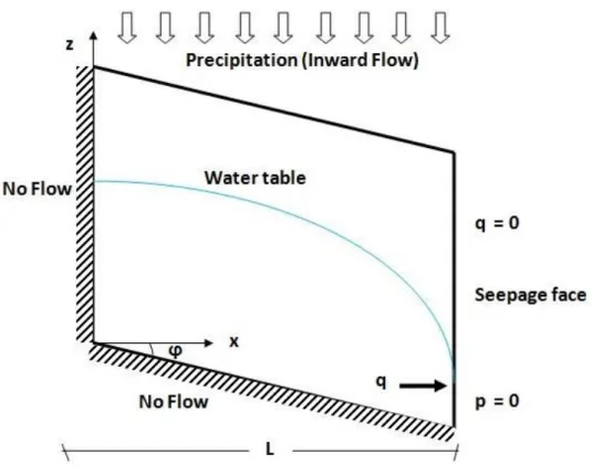
which represents a hillslope flow system, is three dimensional (3D) and spans 5m depth, 20m width and 100m length along the Cartesian coordinate system (XYZ) where Z is directed vertically upward. ... 64 Figure 4.2: Vertical cross section of the 3D flow domain with the boundary

(13)

Università degli Studi Roma Tre xiii

Figure 4.3: Representation of real hillslope with the hypothetical hillslope modelling. The hillslopes are defined as land areas draining either side of the stream reach in each catchment and in the case of headwater sub-catchments (area draining into the source node) an additional hillslope to represent the convergent contributing to a source node. The natural hillslopes are assumed rectangular with hillslope length L along the flow path to the channel. ... 72 Figure 4.4: schematic that illustrates the implementation of the up-scaling

strategy ... 74 Figure 4.5: Location of MOPEX catchments ... 78 Figure 4.6: Elevation map with river network of a) Soquel Creek watershed, CA

b) Council Creek watershed, OK ... 79 Figure 4.7: Sensitivity analysis of the saturated storage for a) the topographic

slope θ, assuming heterogeneous surface soil of 2_{= 1, f = 0, and constant}

recharge qr = 5mmd

-1 _{b) exponential decay parameter f assuming}

heterogeneous surface soil of σ2

= 1, topographic slope of θ = 10°, and constant recharge of qr = 10mmd

-1_{c) the spatial variability of the surface}

soil hydraulic conductivity, assuming slope θ = 10°, f = 0, and constant recharge of qr = 10mmd

-1

... 81 Figure 4.8: The exponent of the power law S – Q relationship curve plotted

against a) topographic slope b) Surface hydraulic conductivity c) exponential decay parameter, and d) surface heterogeneity of the hydraulic conductivity ... 83 Figure 4.9: The exponent of the power law storage – discharge relationship

curve derived from numerical dataset plotted against the predicted value computed from equation (4.11) ... 86 Figure 4.10: The normalized coefficient of the power law storage – discharge

relationship curve plotted against a) topographic slope b) Surface hydraulic conductivity c) exponential decay parameter, and d) surface heterogeneity of hydraulic conductivity ... 87 Figure 4.11: The coefficient of the power law storage – discharge relationship

curve derived from the numerical dataset plotted against the predicted value computed from equation (4.12) ... 89 Figure 4.12: Storage – discharge relationship derived from the closure equations

for synthetic data with variable a) topographic slope ranges 0 to 30º with 5º interval (other variables are Ks=14 ms

-1_{, f = 1m}-1_and

lnks2=1) b)

Hydraulic conductivity Ks ranging from 5 ms

-1_{to 40 ms}-1_{0 with 5 ms}-1

interval (f = 1m-1_,_{θ = 10º and}

lnks2=1) c) f ranging from 0 to 2m-1 with

0.25m-1 _{interval (K}

s=14 ms

-1_,_{θ = 10º and}

lnks2=1) and d) lnk2 ranging

from 0 to 2 with 0.25 interval (Ks=14 ms

-1_,_{θ = 10º and f = 1m}-1

(14)

Università degli Studi Roma Tre xiv Figure 4.13: Hillslope delineation of Soquel Creek watershed (left: accumulation

area threshold of 300) and Council Creek watershed (right: accumulation area threshold of 200) ... 93 Figure 4.14: Mean topographic slope of the hillslopes in Soquel Creek watershed

(left) and Council Creek watershed (right)... 94 Figure 4.15: Hillslope average surface hydraulic conductivity of Soquel Creek

watershed (left) and Council Creek watershed (right) ... 95 Figure 4.16: Storage discharge curve derived from the hillslope modelling for

several values of f ranges from 0 to 1 with 0.1 interval (solid lines) and recession analysis of observed stream flow (dot) a) Soquel Creek b) Council Creek ... 96 Figure 4.17 Spatial distribution of the recession curve parameters a) α b) β c)

the scattered plot of the α values estimated from the bottom-up approach and top-down approach and d) the same as c but for β ... 99 Figure 4.18: Scatter plots of the ratios (theoretical over the empirical/true) of the

coefficients, α, and exponents, β ... 100 Figure 5.1: Vertical cross section of the 3D flow domain. The vertical x1x2

planes located at x2 = 0 and x2 = 20 m are also no-flow boundaries ... 114

Figure 5.2: Cumulative rainfall and outflow for a) rain only case ( in the absence of ET) b) In the presence of ET case. The inserts show the change in the total inflow and outflow volume ... 116 Figure 5.3: Outflow solute concentration obtained from the numerical

experiment a) Rain only case b) Rain and ET case. The inserts show the cumulative flux through the streamflow ... 117 Figure 5.4μ Streamﬂow solute concentration C, observed and predicted by the

TIC model (left) and the total outﬂow mass recovered (right); Period of continuous injection: (a,b) First season (April -June), (c,d) Second season (July — Sep), (e,f) Third season (Oct - Dec), and (g,h) Fourth season (Jan —Mar); Rain only case (RO) ... 131 Figure 5.5μ Streamﬂow solute concentration C, observed and predicted by the

TIF model (left) and the total outﬂow mass recovered (right); Period of continuous injection: (a,b) First season (April -June), (c,d) Second season (July — Sep), (e,f) Third season (Oct - Dec), and (g,h) Fourth season (Jan —Mar); Rain only case (RO) ... 132 Figure 5.6μ Streamﬂow solute concentration C, observed and predicted by the

ESS model (left) and the total outﬂow mass recovered (right); Period of continuous injection: (a,b) First season (April -June), (c,d) Second season (July — Sep), (e,f) Third season (Oct - Dec), and (g,h) Fourth season (Jan —Mar); Rain only case (RO) ... 133 Figure 5.7μ Streamﬂow solute concentration C, observed and predicted by the

TV model (left) and the total outﬂow mass recovered (right); Period of continuous injection: (a,b) First season (April -June), (c,d) Second season

(15)

Università degli Studi Roma Tre xv

(July — Sep), (e,f) Third season (Oct - Dec), and (g,h) Fourth season (Jan —Mar); Rain only case (RO) ... 136 Figure 5.8μ Streamﬂow solute concentration C, observed and predicted by the

TIC model (left) and the total outﬂow mass recovered (right); Period of continuous injection: (a,b) First season (April - June), (c,d) Second season (July - Sep), (e,f) Third season (Oct -Dec), and (g,h) Fourth season (Jan - Mar); Rain and Evapotranspiration case (RET) ... 139 Figure 5.λμ Streamﬂow solute concentration C, observed and predicted by the

TIF model (left) and the total outﬂow mass recovered (right); Period of continuous injection: (a,b) First season (April - June), (c,d) Second season (July - Sep), (e,f) Third season (Oct -Dec), and (g,h) Fourth season (Jan - Mar); Rain and Evapotranspiration case (RET) ... 140 Figure 5.10μ Streamﬂow solute concentration C, observed and predicted by the

ESS model (left) and the total outﬂow mass recovered (right); Period of continuous injection: (a,b) First season (April - June), (c,d) Second season (July - Sep), (e,f) Third season (Oct -Dec), and (g,h) Fourth season (Jan - Mar); Rain and Evapotranspiration case (RET) ... 141 Figure 5.11μ Streamﬂow solute concentration C, observed and predicted by the

TV model (left) and the total outﬂow mass recovered (right); Period of continuous injection: (a,b) First season (April - June), (c,d) Second season (July - Sep), (e,f) Third season (Oct -Dec), and (g,h) Fourth season (Jan - Mar); Rain and Evapotranspiration case (RET) ... 144

(16)

Università degli Studi Roma Tre xvi

List of Tables

Table 2-1: Water retention and conductivity functions for Brooks and Corey model (Brooks and Corey, 1964), and Van Genuchten model (van Genuchten, 1980) ... 19 Table 2-2μ Summary of numerical models of Richards’ equation for unsaturated-

saturated flow (adopted and then modified from Clement et al., 1994 ... 23 Table 3-1: Brooks and Corey parameters for different soil types ... 39 Table 4-1: Summary of the available and source of data for the study areas ... 78 Table 4-2: Model results from some selected subsets of variables estimating the

exponent, b, ranked based on their AICc value from the nonlinear regression models ... 84 Table 4-3: Model results from some selected subsets of variables estimating the

coefficient, a, ranked based on their AICc value from the nonlinear regression models ... 89 Table 4-4: Regression constants present in the closure equations ... 90 Table 5-1: Calibrated model parameters, mean transit time and the mass

recovery corresponds to the first season (Rain only case) ... 134 Table 5-2: Validated model parameters and the mass recovery at for the second,

third and fourth season (Rain only case) ... 137 Table 5-3: Calibrated model parameters, mean transit time and the mass

recovered through the streamflow at the end of the simulation correspond to the first season (RET case) ... 138 Table 5-4: Validated model parameters and the mass recovered through the

streamflow at the end of each simulation corresponds to the second, third and fourth seasons (RET case) ... 143

(17)

Università degli Studi Roma Tre xvii

Acronyms and Abbreviations

DEM Digital elevation model

SSURGO Soil survey geographic dataset

MOPEX Model parameter estimation experiment

NHD National hydrograph dataset

STATSGO United state general soil map

NRCS National resource conservation service

USGS United states Geological survey

TTD Transit time distribution

3-D/2-D/1-D Three/two/one dimensional

HSB Hillslope storage Boussinesq model

CPU Central processing unit

LSM Land surface model

VIC Variable infiltration capacity

AIC Akaike information criterion

(18)

(19)

Università degli Studi Roma Tre 1

1 Introduction

1.1 Background

In hilly and humid forest areas with highly conductive soils, subsurface flow consider as the main mechanism of stream flow generation and responsible for solute transport (eg. agricultural fertilizers and nutrients) into the surface water bodies which is transported through the subsurface soil (Anderson and

Burt, 1990; McGlynn et al., 2003; Sidle et al., 2000; Weiler and McDonnell, 2006; Zuber, 1986). Several studies in the past two decades at different part

of the world (eq. Maimai experiment in New Zealand, Panola mountain research, USA, and other studies) indicated that the pre-event water (which is stored in the subsurface soil before a rainfall occurs) is the dominate contributor of stream flow (Botter et al., 2010; Buttle, 1994; Fiori, 2012;

McDonnell, 1990; Neal and Rosier, 1990; Sklash, 1990; Wenninger et al., 2004) with percentages more than 70% of the total flow. In those field

experiments, hillslopes are fundamental landscape units that control the flow processes where rainfall is transported to streams. Indeed, it is highly important to predict flow, solute transport and land stability at hillslope scale in order to understand the dynamic of hydrological processes and possible governing mechanisms within the subsurface.

Much of the process understanding in hillslope hydrology at steep landscape has studied from field experiments, for example, several studies at the

(20)

Panola mountain research watershed, USA (Clark et al., 2009; Freer et al.,

2002; Lehmann et al., 2006; McGlynn et al., 2001; Tromp-van Meerveld et al., 2008; Tromp-van Meerveld and McDonnell, 2006a, b; Uchida et al., 2005; Wang, 2011); Maimai, New Zealand (McDonnell, 1990; Pearce et al., 1986; Sklash, 1990; Woods and Rowe, 1996; McGlynn et al., 2002) and ,

Hitachi Ohta experimental watershed, Japan (Noguchi et al., 2001; Pearce et

al., 1986; Sidle et al., 2011; Sidle et al., 1995; Sidle et al., 2000; Tani, 1997; Tsukamoto and Ohta, 1988), characterize the enormous heterogeneity and

complexity of surface and subsurface flow processes. However, the ability to employ these ﬁndings to ungauged regions still remains largely out of reach (McDonnell et al., 2007). Parallel to the field experiments, numerical models are increasingly used for studying flow and solute transport at hillslope scale (Bogaart and Troch, 2006; Fiori and Russo, 2007; Harman and Sivapalan,

2009a, b; Lee, 2007; Rocha et al., 2007; Szilagyi et al., 1998; Troch et al., 2003)

Though flow and transport modelling at hillslope scale is receiving much attention in the recent years and different numerical modelling and field experiments have been developed to increase our understanding of flow and transport, a few studies have been done to bring those physical based models to the ground since there is absence of strong techniques of upscaling point based flow and transport equation to hillslope scale and then catchment where mostly water resource development has been carried out. Several issues are also still raised on current generation of subsurface models and remain

(21)

unsolved such as i) the spatial variability of hydraulic parameters, which is not well captured in most analytical models; ii) there is also a fundamental problem in upscaling processes from point to hillslope and catchment scales since Darcy’s based flow equation are initially developed for point scale and could not physically evident to study large scales with average catchment characteristics which exhibit tremendous spatial variability of soil and landscape properties within the catchment ( e.g. soil properties such as hydraulic conductivity); iii) factors controlling the connectivity of hillslope flow (surface and subsurface topography, slope angle, hydraulic conductivity, rainfall intensity etc.); and how these variables affect the connectivity. So far several research works have been carried out to address these issues ( e.g.

Lehmann et al., 2006; Viney and Sivapalan, 2004; Hopp and McDonnell, 2009) and in present work similar issues are also undertaken addressing some

of the components of hillslope hydrology ( such as storage – discharge relationship and solute transport) with an appropriate numerical model.

1.2 General objectives and Scopes

The objective of the present work is to study flow and transport at hillslope scale, and particularly the effect of landscape and soil properties on the subsurface flow generation by examining the storage-discharge curve which is necessary to analyse the contribution of the subsurface flow to the stream. It is also extended to develop a global formulation of a lumped

(22)

storage-Università degli Studi Roma Tre 4

discharge relationship using nonlinear reservoir approach (power-law). This has been started with a simple 2D flow modelling to illustrate the power-law storage discharge curve and the flow recession curve assuming a homogenous system with a quasi - steady flow modelling approach. Then, it is further relaxed with a complex flow modelling of a 3D aquifer with heterogeneous soil properties and variable slope to develop a global closure equation that can be used for ungauged catchments regardless of their characteristics.

In general, each piece of work has their specific objective and has been carried out independently. Chapter 3 aims at the determination of the nonlinear storage-discharge relationship by means of numerical computations using a 2D model. The proposed approach tries to develop simple solutions, with a minimal set of physical parameters, which are as parsimonious and simple as the analytical approaches available in the literature, but relaxing some of the assumptions, like e.g. the boundary conditions and the hydrostatic, Dupuit hypothesis. In Chapter 4, some of the assumptions in the 2D modeling which are physically far from the reality were dropped and certain form of reality was considered (i.e. 3D flow system with heterogeneous soil and landscape characteristics), and extended work has been done to analyze the subsurface flow mechanism. It aims to derive physically based storage-discharge relations as parameterizations of subsurface stormflow, which can be embedded in global land surface models without the need to resolve the flows at smaller scales explicitly. Chapter 5

(23)

evaluates the performance of some categories of solute transport models (both lumped parameter and complex analytical models which requires detail knowledge of the flow velocity and subsurface storage) to reproduce the observed transit time distribution obtained from a coupled flow and transport numerical model at hillslope scale. In this part of the work, all the cases are tested based on the results from numerical experiments (Richards equation) employing three dimensional (3-D) synthetic hillslope dynamic model with real hydrological input (i.e. rainfall) so as the numerical models offer the freedom in full control of all quantities and more realistic subsurface setup.

1.3 Organization of the thesis

The thesis is structured in six chapters which are categorized into three sections. The first section consists of two chapters describe the overall background and literature review. Two sections consists of three chapters describe the flow and transport modelling, respectively and finally conclusion and recommendation closes the thesis. The organization of the thesis with chapters is as follow:

In Chapter 1 the overall background of the research is presented. The overall objectives of the research work and the general flow of the research is also presented in this chapter.

(24)

In Chapter 2, the detailed literature review on Hillslope hydrological modeling with past research works on the area. The flow and transport equation were used in the thesis also presented in this chapter.

In Chapter 3, Numerical modeling of Storage–discharge curves at homogenous hillslope is presented with the perspective of the model parameters to develop the relation Q(S) (where Q is the discharge and S is the saturated storage in the hillslope), as a function of some simple structural parameters.

In Chapter 4, 3-D numerical modelling of the storage discharge curve is analysed and physically based parameterizations of the storage-discharge relationship relating to subsurface flow are developed. These parameterizations are derived through a two-step up-scaling procedure; point to hillslope scale and then to catchment scale employing simple and robust upscaling approach. This parameterization is also applied for 50 catchments in the United State and compared with the same parameters found empirically from observed data.

In Chapter 5, performance of solute transport models using traditional lumped parameter based TTD and a comparable analytical model routes the inflow concentration into outflow to reproduce the observed transit time distribution obtained from tracer study using a numerical experiment at hillslope scale with and without the presence of evapotranspiration is evaluated and the preference of each modeling approach is presented.

(25)

In Chapter 6, the overall summary of the research with some concluding remarks are given. The limitations and some assumptions made during the research are presented in this chapter.

(26)

(27)

2 Subsurface Flow and Transport at Hillslope scale:

Theoretical overview

2.1 General overview of Hillslope Hydrology

“One of the aims of hillslope hydrology is to explore the process complexity

underlying watershed responses through carefully constructed field experiments in selected hillslopes, and through detailed numerical models that are able to capture key or dominant processes and which, in turn, are validated by the field observations.” (Sivapalan, 2003).

In most hydrological models at catchment scale, flow and transport are generally modelled in a lumped or distributed mode. The distributed models are often divide large catchment into small homogenous units that are supposed to have uniform characteristics (Sivapalan, 2003) whereas lumped models consider an entire catchment as one unit, characterized by a small number of parameters and variables which are uniform and spatially averaged over the catchment ( e.g. mean areal rainfall). However, due to the large multi-scale heterogeneities that nature exhibits, it is uncertain to study processes using such lumped at a scale in which the spatial heterogeneity is fairly represented (Watson et al.,2001) and conversely, the fully explicit distributed models represent sufficiently but are data demanding. Thus, this spatial scale within the models which is more appropriate with our

(28)

understanding of the hydrological processes and the dominant controlling factors can be modelled at the hillslope scale (Fan and Bras, 1995).

Hillslope scale hydrological models based on the flow equation are the most essential approach to quantify hydrological responses for both gauged and ungauged catchments. It can also easily handle the dynamic characteristics of the flow and transport processes which results inexpensive respect to both conceptual and computational complexity. In fact, it is clear that physical equation explains flow through homogenous media at the point scale, but does not explain processes at large scale such as effect of variable soil properties and bed rock properties on subsurface flow through soil macropores (Beven and Clarke, 1986; Freer et al., 2002; Tromp-van

Meerveld and McDonnell, 2006a) . As such, applying hydrological models at

the large scale requires estimating equivalent soil and landscape parameter values that can represent the overall properties. Although such approach has been used to study hydrological processes at catchment, there are several factors that limit the application of the homogenous equivalent physical-based models over large areas (Beven, 2002). First, an increase in modelling scale is usually accompanied by an increase in the variability of physical properties (such as soil and topography) at different ranges of space (Figure 2.1). Averaging these catchment properties is not commensurate with the reality and may provide inappropriate modelling responses when applying for a complex spatially variable catchment. Second, some models evolve very complex approach to capture flow processes at the hillslope scale (e.g.

(29)

macropore flow), but an incomplete description of processes at the watershed scale (e.g. subsurface flow interaction with streams) (Clark et al., 2009). Finally, detail large scale (catchment scale) process-based models often have large computational requirements even though there are advanced computer hardware technologies to make detailed simulations at large scale. It is therefore, hillslope scale models are recently being developed and scientifically recognized to overcome such limitations (Ali et al., 2013;

Anderson and Burt, 1990; Brooks et al., 2004; Burns et al., 1998; Fiori and Russo, 2008; Graham and McDonnell, 2010; Harman and Sivapalan, 2009b; Harman et al., 2010; Hopp and McDonnell, 2009; Uchida et al., 2005; Wenninger et al., 2004)

Figure 2.1: Variability of catchment and hydrological processes at a range of space scale (Blöschl and Sivapalan, 1995)

(30)

Different hillslopes in a catchment generate runoff at different timing and amount during a storm even since they have different topographic and landscape properties. These hillslopes are integrated by the river channel where they are contributed and which make a catchment with a single outlet so that areas outside of the river channel in a catchment are considered as hillslope (Figure 2.2), even they are completely flat (hillslope with zero slope). Therefore, in several hydrological models hillslopes are taken as a computational unit for both surface and subsurface flow modelling in order to capture all the hydrological processes with fair representation of the soil heterogeneity and topographic slope. It is clear that insight into the hydrological processes at hillslope scale and the effect of the variability of hydraulic characteristics of landscape elements is required to further our understanding and ability to model catchment hydrological processes.

(31)

Figure 2.2: Schematic view of catchment with its hillslope units and hillslope discretization scheme (the arrow indicates the flow direction to the streams)

Several models have been developed over the past decades to quantifying the flow processes employing different flow equations and modelling approaches. Among these modelling approach, the most widely used models involve numerically solving are based on Richard’s equation (Paniconi and

Wood, 1993). However, these models are very complex and demand high

computational effort. Indeed, there are other models recently used which avoid such model complexity by adopting some basic assumptions in which the three-dimensional soil mantle of complex hillslopes with variable width

(32)

are collapsed into a one-dimensional drainage pore space (Fan and Bras,

1998; Troch et al., 2002; Troch et al., 2003). For example, Troch et al. (2004) presented an analytical solution of the linearized HSB equation for

exponential hillslope width functions. Analytical solutions like these provide essential insights in the functioning of hillslopes and may form the basis of hillslope similarity analysis (Brutsaert, 1994). Though, such models are practically easy to simulate subsurface flow and storage with less cost, they are based on analytical solutions to the Boussinesq equation assuming equivalent representative values of catchment properties (e.g., Brutsaert and

Nieber, 1977;Brutsaert and Lopez, 1998; Rupp and Selker, 2005, 2006) and

the effects of heterogeneity of topographic gradient and soil hydraulic properties within hillslopes and catchments are not well captured. It is therefore essential to employ three dimensional model of Richards’ equation so that the actual effect of soil and landscape variability can be embedded implicitly in the numerical models. Details of the Richard’s equation and methods used to solve Richard’s equation are discussed in the next sections.

2.2 Governing Flow and Transport Equations

In this section, the fundamental flow and transport equations used in the present work are summarized. Mathematical equations that describe the subsurface flow and transport processes may be developed from the fundamental principle of continuity equation and conservation of mass of fluid or of solute. Accordingly, the mathematical background and basic

(33)

assumptions employed in the Richards’ equation (flow equation) and the convection-dispersion equation (solute transport equation) are discussed in this section.

2.2.1 Subsurface flow equation: The Richard’s equation The recognized physical model for the subsurface flow of water is the three dimensional (3D) Richards’ Equation (Richards, 1931). It is very useful to analyse soil water fluxes in variable saturated soils and able to solve the strong nonlinearity of soil hydraulic functions.

Figure 2.3: Darcy’s law experiment

h1 1 z1 h2 1 z2 Δh = h1-h2 Datum level Q A Sand

(34)

Starting from the Darcy’s law experiment shown in Figure 2.3 which relates the flow velocity

q

to the hydraulic conductivity

K

and the pressure head inside the flow system

h



h z



K

q   (2.1)

with

z

denotes the vertical coordinate in the medium. The continuity equation in unsaturated soils 0      q t  (2.2) combined with Darcy law in equation (2.1) leads to Richards’ equation

0 )) ( .(        z h K t  _(2.3)

Different mathematical models used the Richards equation in equation (2.3) that made used to describe variable saturated flow and derived by combing the Darcy’s law with the continuity equation in porous media so that the hydraulic conductivity depends on water content and pressure head. There are generally three main form of Richards’ equation presented in the literature namely the pressure head (h) based formulation, water content (θ) – based formulation and mixed formulation (Celia et al., 1990; Azizi et al., 2011). Pressure based 0 ) ( ) ( ) (           z h K h h K t h h C (2.4)

(35)

Water content based

0 ) ( ) (           z K D t     (2.5) Mixed form 0 ) ( ) (           z h K h h K t  (2.6) where h is the pressure head (L), z is the vertical coordinate (L), θ is the volumetric water content, C(h)



h is the specific moisture capacity (1/L), K(θ or h) is the hydraulic conductivity ( L/T), D(



)K(



) C(



)is the diffusivity (L2/T) and t is time (T).

The θ-based form cannot be used for the simulation of unsaturated-saturated flow and might generate significant local numerical errors for a coarse grid near interfaces with abrupt permeability changes, where heterogeneous porous media are concerned (Zaidel and Russo, 1992). The h-based form is not conservative and, as a result, cannot be used with reasonable time steps, especially for modelling infiltration into relatively dry soils. The mixed form of Richards' equation (Celia et al., 1990) has been provided attractive representation of the unsaturated- saturated flow and so, we will focus on this form of the flow equation.

(36)

The water content and the soil water potential may be related together through the use of an empirical function called water retention curve, which states that for a specific moisture level there is a defined value for suction.

Figure 2.4: Soil water characteristic curves for selected soils ranges from sand to clay (Tuller

and Or, 2004)

The shape of the water retention curves depends on the pore size distribution of the soil and exhibit different suction ranges for different soil since capillary forces are getting larger for finer textured soils (see Figure 2.4). Several models have been developed in order to describe the water retention curve and the Richards’ equation can be solved. Brooks and Corey’s model (Brooks and Corey, 1964) and Van Genuchten model (van Genuchten, 1980) are among the widely used models. The Van Genuchten model uses mathematical relations to relate soil water pressure head with water content

(37)

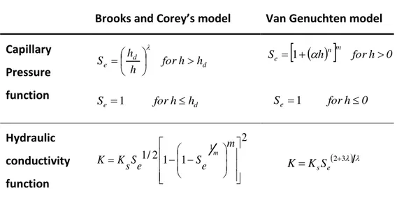
and unsaturated hydraulic conductivity. This model matches experimental data but its functional form is rather complicated and it is therefore difficult to implement it in most analytical solution schemes whereas Brooks and Corey’s model has a more precise formulation. Table 2.1 indicates water retention and conductivity function for Van Genuchten and Brooks and Corey models.

Table 2-1: Water retention and conductivity functions for Brooks and Corey model (Brooks

and Corey, 1964), and Van Genuchten model (van Genuchten, 1980)

Brooks a d Corey’s odel Van Genuchten model

Capillary Pressure function d d e forh h h h S          d e forh h S 1 

 



h



forh 0 Se  1  n m  Se 1 forh0 Hydraulic conductivity function m e S e S s K K m 2 1 1 2 / 1 1                        S K K _s _e23 

Notations: h is capillary pressure head; h_d is the air entry pressure head;  is pore size distribution index; S_e is effective saturation; Kis the hydraulic conductivity at specific water saturation; K_sis the saturated hydraulic conductivity; and n are the Van Genuchten model parameters.

(38)

Several research works have been done to provide numerical and analytical solution of Richards’ equation in order to simplify and easily implemented for field soils with some sort of assumptions. In recent years, semi-analytical methods have been developed for Richards’ equation (Srivastava and Yeh,

1991; Elnawawy and Azmy 1992; Marinelli and Durnford, 1998; Hogarth and Parlange, 2000; Lu and Zhang, 2004; Menziani et al., 2007). These

analytical solutions of the Richards’ equations are an excellent tool to solve simple subsurface flow problems such that the nonlinear Richards’ equation should be converted to a linear form even though it is highly non-linear and unlikely valid for complex conditions. Tracy (2006) obtained multidimensional solutions to the Richards equation in which the quasi-linear approximation combined with relative hydraulic conductivity varying exponentially with pressure head. This combined result with Kirchoff’s transformation and the moisture content which is also varying linearly with relative conductivity allows the linearization of Richards’ equation for both steady and unsteady flow simulation. Basha (2000) has also produced multidimensional analytical solutions for unsteady infiltration towards a shallow water table using the same approximation. There are methods to transform and separate variables. For example, Basha (2000) uses Green’s functions to obtain the multi-dimensional solutions. Boltzmann similarity transformation is also used for 1D Richards’ equation that converts the partial differential equation (PDF) to an ordinary differential equation (ODE) (Logan, 1987). Other methods are Laplace and Fourier transformation (Fityus

(39)

Since the subsurface flow condition is highly nonlinear due to the extent of the non-linearity in hydraulic properties, multidimensional nature of water flow and pressure relationships of media; numerical methods combined with some iteration schemes are typically used to solve the Richards’ equation (Celia et al., 1990; Paniconi et al., 1994; Fiori and Russo, 2007). However, they are usually computationally expensive and cannot be used to model large catchments. Thus as we discuss earlier, it can be minimized the computational cost using small scale problems necessarily to study detail hydrological processes followed by upscaling.

Once the form of the flow equation has been chosen one must select the solution procedure. Since analytical solutions for the Richards’ equation are known for simplified situations only, thus for more involved situations, numerical methods which are preferable in view of the reliability of the computed solutions. The numerical methods which are employed to solve Richards’ equation are a finite difference, a finite element and a finite volume method. Even though there are several research works have been carried out on the convergence properties of these methods to improve the physical discretization of these standard solutions, comprehensive analyses on the accuracy and efficiency of such methods in heterogeneous formations have not been performed so far. This aspect is particularly important in highly heterogeneous formations, such as those encountered when considering flow along hillslopes. The numerical discretization of the Richards’ equation in

(40)

this study has been discussed in the later section. Table 2.2 indicates some previous research works that have been developed using Richards’ equation based on different formulation and numerical discretization

(41)

Table 2-2μ Summary of numerical models of Richards’ equation for unsaturated- saturated flow (adopted and then modified from Clement

et al., 1994

Model Subsurface Flow Equations Solution procedures

FEMWATER (Yeh, 1981) h-based 2D variable saturated flow Finite element; with Gauss elimination 3D FEMWATER (Yeh, 1992) h- based 3D Richards equation Finite element; with Gauss elimination Cooley (1983) h–based 2-D variable saturated flow Finite element; combination of

Newton-Raphson and strong implicit

Allen and Murphy (1986) Mixed form of Richards’ equation Collocation finite element; Gauss elimination

VS2DT (Healy, 1990) h-based form of general variable

saturated flow ( 2D)

Finite difference; strong implicit procedure

Hydrus Model (Simunek et al., 1996) Mixed form of Richards’ equation Galerkin-type finite element

MODHMS (Panday and Huyakorn, 2004) Mixed form of 3D Richards’ equation Block centred Finite difference scheme GSSHA model ( Downer and Ogden, 2004) h- based Richards’ equation Implicit finite difference

WASH123D(Yeh et al., 2004; Yeh et al., 2006)

3D Richards equation Finite element method

Fiori and Russo (2007) Mixed form of 3D Richards’ equation Finite difference, implicit procedure based on nodes distribution

(42)

Università degli Studi Roma Tre 24 2.2.2 Governing Transport Equation

Solute transport occurs in the subsurface system through the combination of diffusion and advection. The convection-dispersion equation (CDE) considers the solute flux to be the result of the average bulk motion of the solute in the direction of subsurface flow (advection) and a Fickian-type mixing between the original and displacing fluid (dispersion) (Gillham et al., 1984). For unsaturated - saturated flow in isotropic heterogeneous porous media, the governing equation is written as,

 

_

_{  }

c u c D t c _ _  ___ _ __   (2.7)

where cis the solute concentration expressed as mass per unit volume; u

is the flow velocity and D is the hydrodynamic dispersion tensor. The dispersion tensor for isotropic media is given as (Bear, 1972)

Dij Tuij 



L T



uiuj u Dˆij (2.8) where



_Tand



_Lare transversal and longitudinal pore scale dispersivities ; _ij is the Kronecker delta (i.e. _ij 1, if i jand _ij 0, if i j); uis

the magnitude of mean flow velocity in the subsurface and expressed as



2 2 2



12

z y

x u u

u

u    ; Dˆ is the molecular diffusion coefficient and the

diffusion term is mostly is assumed zero since the mechanical dispersion is much larger than the diffusion term.

(43)

2.3 Recession flow analysis

Recession flow analysis is the well-known tool in hydrology and has several applications to characterize the low flow in a stream provides information concerning the availability of water resource to benefit the planning and management of water related projects such as irrigation, water supply and hydropower plants (Tallaksen, 1995). It also used to conceptualize the subsurface storage parameters and estimate aquifer characteristics of a catchment (Moore, 1992; Lamb, 1997).

Figure 2.5: Defination sketch for the Dupuit – Boussinesq aquifer model ( Brutseart and Nieber, 1977)

On the basis of different approaches, several types of models to describe recession flow have appeared in the literature. In one type of approach,

Horton (1933) suggested the nonlinear relationship of the outflow

discharge as ( ) 0exp( )

m

at Q

t

Q   , where Q₀is the initial discharge, a

(44)

Università degli Studi Roma Tre 26 discussed based on a simple flow equation by Werner and Sundquist

(1951); Tallaksen (1995). Other methods such as modelling recession as

reservoir (Barnes, 1939; Fenicia et al., 2006; Aksoy and Wittenberg,

2011; Chapman, 1997; Harman and Sivapalan, 2009b; Wittenberg, 1999; Wittenberg and Sivapalan, 1999), using regression equation ( James and Thompson, 1970; Vogel and Kroll, 1992) and empirical relationships

(Radczuk and Szarska, 1989;Clausen, 1992) are among the most widely used approaches.

Boussinesq (1877) introduced non-linear differential equation for

unsteady flow from unconfined aquifers to a stream channel by considering the Dupuit assumptions which neglects the vertical flow component and also neglecting the effect of capillarity, groundwater recharge and evapotranspiration (Brutsaert and Nieber, 1977). Theoretical equations for groundwater flow derived from the Boussinesq equation have been presented by Brutsaert and Nieber (1977). They have proposed to determine the outflow rate from low flow hydrograph derived from direct measurements ofQ(t)and nonlinear Dupuit Boussinseq aquifer model (Figure 2.5) is developed and the parameters for the lumped storage model are determined. This low flow analysis has been extensively applied by various researchers. The storage model they have employed has the form of a power function f Q Q

dt

dQ _ ₍ ₎__ _where

α and are constants and can also be obtained from the Dupuit

Boussinesq aquifer model by assuming some geometrical similarity of the catchment. Alternatively, the same equation is obtained after combining the non-linear storage–discharge relationship, b

aS

(45)

Università degli Studi Roma Tre 27 continuity equation of a reservoir without inflow, Q

dt

dS __ _{. This}

approach allows developing parameterizations using an inverse procedure, from catchment runoff measurements that already account for the net effects of natural variability of soil and topographic properties. This is based on the relationship between the storage-discharge relationship and the shape of the recession curve extracted from observed streamflow records. It can be shown that the parameters a and b of the storage-discharge relationship are uniquely related to the parameters  and  associated with the recession slope curves which is  a1/bb and

b

1

2 

(46)

(47)

3 Analysis of the nonlinear storage

– discharge

relation for hillslopes through 2D numerical

modeling

1

Abstract:

Storage–discharge curves are widely used in several hydrological applications concerning flow and solute transport in small catchments. This article analyzes the relation Q(S) (where Q is the discharge and S is the saturated storage in the hillslope), as a function of some simple structural parameters. The relation Q(S) is evaluated through two-dimensional numerical simulations and makes use of dimensionless quantities. The method lies in between simple analytical approaches, like those based on the Boussinesq formulation, and more complex distributed models. After the numerical solution of the dimensionless Richards equation, simple analytical relations for Q(S) are determined in dimensionless form, as a function of a few relevant physical parameters. It was found that the storage–discharge curve can be well approximated by a power law functionQ LKs a



S L ( r)



b

2 ___

 , where L is the length

of the hillslope, Ks the saturated conductivity,







rthe effective

porosity, and a, b two coefficients which mainly depend on the slope. The results confirm the validity of the widely used power law

1

Adapted from Ali, M., A. Fiori, and G. Bellotti (2012). Analysis of the nonlinear storage--discharge relation for hillslopes through 2D numerical modelling. Hydrol. Process., doi: 10.1002/hyp.9397

(48)

Università degli Studi Roma Tre 30 assumption forQ(S). Similar relations can be obtained by performing a standard recession curve analysis. Although simplified, the results obtained in the present work may serve as a preliminary tool for assessing the storage–discharge relation in hillslopes.

(49)

3.1 Introduction

The storage-discharge relation is a very important component of catchment hydrology and it is widely used for several engineering applications, such as estimating design floods (Rahman and Goonetilleke,

2001), forecasting of low flows for water resource management (Vogel and Kroll, 1992), estimating groundwater potential of basins (Wittenberg and Sivapalan, 1999) and rainfall runoff models (Sriwongsitanon et al., 1998). The matter has been investigated in the framework of base flow

recession, hydrograph separation and other related areas of hillslope hydrology (Brooks et al., 2004; Fiori and Russo, 2007; Graham and

McDonnell, 2010; McGuire and McDonnell, 2010; Weiler and McDonnell, 2004). Based on different principles and approaches, the

recession of subsurface flow has been studied by Brutsaert and Nieber

(1977);Wittenberg (1994); Wittenberg (1999); Fenicia et al. (2006), Aksoy and Wittenberg (2011); Wang (2011); Moore (1997). Tallaksen (1995) has discussed various methods and approaches widely used to

determine the storage discharge relationship by the recession curve analysis.

One of the widely employed storage-discharge relations is the linear reservoir model, originally defined by Maillet (1905), which implies that the aquifer behaves like a single reservoir with storage S, linearly proportional to outflow Q, namelyQaS. In this case, the plot of logQ_t

against S yields a straight line (Barnes, 1939). Moreover Fenicia et al.

(2006) have also derived actual S-Q relation in which the percolated water

(50)

Università degli Studi Roma Tre 32 to the saturated reservoir are taken into account, for which the S-Q relation was treated as a linear and second order polynomial. However, linear reservoir (QaS ) can very well describe the groundwater

behavior for most of the catchments they have studied. In most real cases however, semi-logarithmic plots of flow recessions are still concave (Aksoy and Wittenberg, 2011), indicating nonlinear storage discharge relationships.

Recent studies agreed that the outflow of a lumped storage model can be characterized by a general power law function b

aS

Q where a and b are

constants. The constant b varies between 0 and 2 or higher for some cases (Chapman, 1997; Harman and Sivapalan, 2009b; Wittenberg, 1999;

Wittenberg and Sivapalan, 1999) and also it has been proved by physical

experiments (Chapman, 1999; Wittenberg, 1994). The power law formulation is only occasionally chosen in recession analysis (Wittenberg,

1994), and the recession process is commonly formulated in terms of the

reservoir inflow and outflow, which can be calculated using the continuity equation.

On the other hand, Brutsaert and Nieber (1977) have proposed to determine the outflow rate from low flow hydrograph derived from direct measurements ofQ(t). They have developed their models based on the nonlinear Dupuit Boussinseq aquifer model and determined the parameters for the lumped storage model. This low flow analysis has been extensively applied by various researchers. The storage model they have employed has the form of a power function QaS f Q Q

dt

(51)

Università degli Studi Roma Tre 33 where α and are constants and can also be obtained from the Dupuit

Boussinesq aquifer model by assuming some geometrical similarity of the catchment. From the solution for the outflow rate they have estimated

1=3 and 2=3/2 for short time and long time solution respectively.

Recently Wang (2011) has used the method proposed by Brutsaert and

Nieber (1977) at the Panola Mountain Research Watershed, Georgia. The

work has elaborated more on the effect of groundwater leakage and return flow on the recession curves. On his work he has studied the recessions for three nested hillslopes and watersheds and estimated recession slope curves (RSC) for different values of a and b based on the observed data for the three watersheds at the Panola mountain.

Parallel to the analytical approximation for computing hillslope subsurface flow, numerical models are increasingly used for computing the recession flow and baseflow analysis, and also for comparison with the analytical approximation (Lee, 2007; Rocha et al., 2007; Szilagyi et

al., 1998). For example Lee (2007) develops a recession model that can

provide the theoretical basis of subsurface modeling using dimensionless Richard’s equation, treating both saturated and unsaturated flow domains. The use of the storage-discharge relationship, together with the continuity equation, resembles other similar approaches in hydrological modeling, like e.g. the kinematic model for flood propagation. In essence, the dynamic equation is simplified by a quasi-steady state relation between storage and discharge. The same approach was employed by Kirchner

Subsurface flow and transport modelling at the hillslope scale

UNIVERSITY OF ROMA TRE

Faculty of Engineering

Doctoral School of Engineering

Civil Engineering Section

PhD in Civil Engineering

XXVI Cycle

Doctoral Thesis

Subsurface Flow and Transport Modelling at the Hillslope

scale

Roma,

April 2014

Doctoral School of Engineering/PhD in Civil Engineering

SCUOLA DOTTORALE / DOTTORATO DI RICERCA IN

XXVI

CICLO DEL CORSO DI DOTTORATO

Subsurface Flow and Transport Modelling at the Hillslope

scale

________________________________________________

Titolo della tesi

Melkamu Ali __________________

Nome e Cognome del dottorando

Prof. Aldo Fiori

__________________

Docente Guida/Tutor: Prof.

Prof. Aldo Fiori

__________________

Subsurface Flow and Transport Modelling at the Hillslope

scale

Abstract

Acknowledgements

Subsurface Flow and Transport Modeling at

the Hillslope scale

Table of Contents

List of Figures

List of Tables

Acronyms and Abbreviations

1

Introduction

1.1 Background

1.2 General objectives and Scopes

1.3 Organization of the thesis

2

Subsurface Flow and Transport at Hillslope scale:

Theoretical overview

2.1 General overview of Hillslope Hydrology

2.2 Governing Flow and Transport Equations

q

K

h





z









 





 



  













2.3 Recession flow analysis

3

Analysis of the nonlinear storage

– discharge

relation for hillslopes through 2D numerical

modeling









3.1 Introduction

_

_{  }