Analysis of Dynamic PET Data for Reversible Tracers of Neuroreceptor Studies

____________

Analysis of Dynamic PET Data for Reversible Tracers of Neuroreceptor Studies

Advisor: Ignasi Juvells and Xavier Pavía.

Facultat de Física, Universitat de Barcelona, Diagonal 645, 08028 Barcelona, Spain.

Abstract: [18F] FDDNP is a tracer used in positron emission tomography (PET) studies to evaluate amyloid plaques deposits in different types of neurological disease. In a standard study an image sequence is acquired during 90 min post injection. This study suggests an analysis method to quantify the dynamic study and evaluates the differences among patients. Programs have been developed and various parameters have been optimized to increase the reliability of the results.

I. INTRODUCTION

PET is an imaging technique that produces 3D functional images of a physiological process. PET images give information about the distribution of the radioactive tracer in in a certain part of the body. The PET camera detects the two gamma rays emitted by the positron emitter nuclide in the radiotracer.

Magnetic resonance tomography (MRT) images are available in the study. These images provide anatomical information of the brain such as the grey and white matter locations.

A dynamic PET sequence is performed obtaining in this way different PET images over a period of time (so it will be a 4D study). In order to analyse this time sequences, we must apply compartmental models. These models are simplifications of the real physiology, but they provide an estimation of the model parameters of the subjects. (Fig.1)

FIG. 1: Schematic representation of a two compartmental

model, where Cp(t) is the input function (plasma concentration), and

the other two compartments have their own concentrations curves. k1, k2, k3, k4, are rate constants of the compartments.

In our research, PET images were obtained using [18F] FDDNP (2-(1-{6-[(2- [fluorine-18] fluoroethyl) (methyl) amino]-2- naphthyl} ethylidene) malononitrile). This tracer has different binding properties in amyloid plaques and neurofibrillary tangles, higher in cases. [1]

There are 2 types of tracers, reversible and irreversible. Reversible tracers are those that can return to a previous compartment. Irreversible are those that cannot do it. [18F] FDDNP is a reversible tracer.

A. Graphical methods

For reversible tracers, in general, compartmental equations can be written like:

𝑑𝐶̃

𝑑𝑡 = 𝐾̃𝐶̃ + 𝑄̃𝐶𝑃(𝑡), (1) where 𝐶̃ is the vector of compartmental concentrations at time t, 𝐾̃ is a matrix of the transfer constants between compartments, 𝑄̃ is a vector of plasma to tissue transfer constant, 𝐶𝑃(𝑡) is plasma concertation of unmetabolitzed

tracer (input function).

If we define ROI (region of interest) like: 𝑅𝑂𝐼(𝑡) = 𝑈̃𝑛𝜏𝐶̃ + 𝑉𝑝= ∑ 𝐶𝑖(𝑡)

𝑖

𝑉𝑝, (2)

Where ROI represents the sum of radioactivities from all compartments and includes plasma volume fraction (𝑉𝑝). 𝑈̃𝑛𝜏

is the transpose of the vector of 1’s that allows the sum of radioactivity. Integrating Eq. (1), multiplying by 𝑈̃𝑛𝜏 and

rearranging we have: ∫ 𝑅𝑂𝐼(𝑡𝑡 ′_)𝑑𝑡′ 0 𝑅𝑂𝐼(𝑡) = 𝐷𝑉𝑅 ∫ 𝑅𝐸𝐹(𝑡𝑡 ′_)𝑑𝑡′ 0 𝑅𝑂𝐼(𝑡) , (3)

Where 𝑅𝐸𝐹(𝑡′_{)𝑑𝑡′ represents a region where the amyloid}

plaques did not change drastically, in our case the cerebellum. DVR (distribution volume ratio), is a model parameter that gives us information about how the tracer is binding to the tissues.

We are going to use graphical methods to get the DVR. If we plot ∫ 𝑅𝑂𝐼(𝑡 ′_)𝑑𝑡′ 𝑡 0 𝑅𝑂𝐼(𝑡) versus ∫ 𝑅𝐸𝐹(𝑡₀𝑡 ′)𝑑𝑡′

𝑅𝑂𝐼(𝑡) , we will get a line, the

slope of which will be our DVR and the number of points is given by how many 𝑡 we have [2] [3] [4].

In most cases, plotting the above mentioned will not get a perfect line, bending in the first points of the line. We will discuss later how many points should be keep for making the DVR.

The purpose of this paper is to analyze and implement the graphical method to determine DVR. The most important point is to discuss how many points we keep to get an accurate assessment of DVR.

II. MATERIAL AND METHODS

A. Material

It consists of four MRT images (Fig.2) with their respective dynamic PET images (Fig.3), captured during 65 minutes, and 15 frames, captured with a shorter interval at first, and spaced at the end. Every pixel shows a proportional number to the amount of tracer fixed on the correspondent tissue. There are two cases with PD and AD (cases 2 and 5), one with PD (case 16) and one control case (number 15), with no mental disease.

FIG. 2: Orthographic projections of a MRT image.

FIG.3: Orthographic projections of a PET image. This image

has been made summing all the intervals of one case.

B. Software

Matlab was used for develop the software. SPM8 (Stastical Parametric Mapping) which run’s on Matlab too, was also used, adapted to our case, for quantify and determinate the AAL and the gray matter.

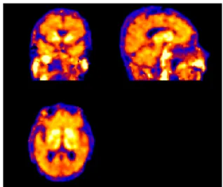
The program it is divided in two parts, the output of first part is a DVR image for each case. That output is a brain image, which each pixel is the value of the DVR (Fig.4).

FIG. 4: Orthographic projections of a DVR image.

The second part, takes the result of the previous, and makes the corregister, quantify the AAL and get which zones is gray matter.

C. Quantification

Once we have the DVR image, some method is needed to compare different cases, not just with a visual observation. Amyloid plaques are located mainly in the gray matter, so we need to separate it from white matter.

First of all, the space (coordinate system) where the DVR is, is the same that the space of the PET image. But this space is not the same as the MRT images. We need to put the 2 images in the same space (we will work on the MRT space), this can be done because the physical volume is the same, so it only needs the application of rotations, translations or scale factors. This process is known has corregistration.

Now that MRT and DVR images are in the same space, we have to know the transformation (T) to normalize and bring it to the standard space, where there is the information about the brain. Segmentation of the MRT is done at this point, which consists in getting a map of the gray matter (Fig. 5) in the standard space.

In this space there is the division of the brain too, all the divisions are named AAL [1] (Automated Anatomical Labeling) in other words, AAL projects divisions in the brain atlas onto brain-shaped volumes of functional data. It contains white and gray matter.

Once we have our T, T-1 is applied to the areas of gray matter and AAL, which are in the standard space, to bring them into the RM space, and consequently to the DVR space. The overlapped areas of gray matter and AAL will be the zones that we will focus on our research. Quantification consists of getting all the DVR values of these overlapped areas, usually the mean of each area.

FIG. 5: Orthographic projections of the gray matter areas.

D. Integral method

First of all, eq. (1) has some integrals and functions evaluates at specific time. But we are working with images, not with normal functions, that can be solved analytically. So we must know what kind of data we have. PET images are the sum of all radioactive decays over a period of time. So it can be used like the integral itself. The value of a singular time 𝑅𝑂𝐼(𝑡) is also needed, so we just take the value of the integral, and divide it for the time interval.

Now, it should be discussed which time value is taken. If we just take the value of the integral and the value we before divided by the interval, it will be a mistake, because the value of the average value is in the middle of the interval, and not at the end, where the time is.

The problem can be solved, taking every time half of the previous integral and half of which we are evaluating (Fig.6).

FIG. 6: Schematic representation of the method used for eq.(3).

In this way the value of the integral and the point are evaluated at the same time.

E. Determination of ideal number of points One purpose of this paper is to determine the optimal number of points of the slope (DVR) in eq. (3). The number of points is given by how many intervals the dynamic PET has, in our case, 20. If we take all the points, the straight folds in the firsts (Fig.7).

FIG. 7: Grafhical analysis of the eq.(3).

A method is needed to discriminate how many points we take, if all points are taken, the resultant slope it would not have been made with a real straight, if too few points are preserved, we will lost some information, and the error could increase due to lack of points.

First of all we make 20 DVR images, using 20 to 1 points of the straight for each case (removing the firsts points first, so on until the last). One of these 20 images will be the one we are looking for. Then we subtract the first image with his after and doing this with all of them. These images are now the changes between one image and his after. Then we will do the statistic deviation of them (Fig.8). We want to search the zone of points with minimum values.

FIG. 8: Graphical view of the standard deviation on the

We can calculate the mean of the subtract images (Fig. 9). When plot crosses the abscissa axis, it will be the point that two consecutive images doesn’t change.

FIG. 9: Graphical view of the mean on the subtracted images.

With Fig. 8 and Fig. 9 it can be seen that the zone between 6 and 12 points it is more plausible to found the ideal number of points.

F. Determination of interest regions There are 112 AAL zones, but not all of them are valid for seeing changes in amyloid plaques. We will focus on some regions, which are composed of several AAL [1] [5]. The overlap areas, between regions (Frontal, Parieto-Occipital, Temporal lateral and Striatum) and gray matter will be the zones that we will focus our research.

III. RESULTS

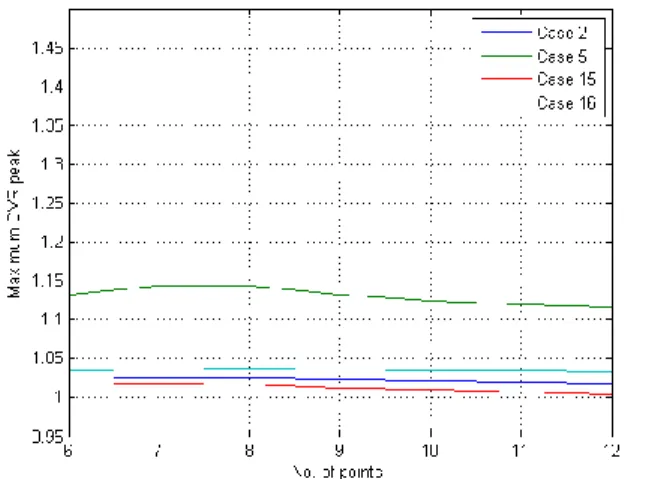
It can be seen in Fig. 10 that the case with lower DVR is case 2. In the other figures, the case with lower DVR is case number 15.

FIG. 10: Plot of the maximum DVR peak for diferent cases, of

the Frontal region.

FIG. 11: Plot of the maximum DVR peak for diferent cases, of

the Paricto-Occipital region.

FIG. 12: Plot of the maximum DVR peak for diferent cases, of

the Temporal lateral region.

FIG. 13: Plot of the maximum DVR peak for diferent cases, of

the Striatum region.

In Fig.11, the variation of every value is very little, similar to 0.1. In Fig.12 the variation is a bit higher, and in Fig.13 the variation is almost 0.5.

The previous figures are made with the peak values of each region and not the mean, which seems to be the more standard choice. This decision was taken because maybe the most important thing is not the mean of the entire region but

the highest value. This can work because the region could not be centred enough in the area peak, and the outer regions of the pick are outside of our AAL and they are not counting to the mean. If we take only the value of the pick, this problem can be solved.

In every case, the differences between numbers of points taken are almost negligible, but between numbers 7 and 8, the differences in Fig. 11 and Fig. 13 are bit higher.

IV. CONLCUSIONS

 A software for getting the DVR image has been done using Matlab.

 A SPM program has been adapted and done for quantify, normalize and calculate the AAL and the gray matter regions.

 A method for calculating point values and integrals from eq. (3) for the correct calculation of DVR has been done.

 We have determined the number of optimal images for the calculating of DVR, between 6 and 12, and more specifically, between 7 and 8.

 This method has been tested with 4 real cases, 3 with neuronal pathology and one with any pathology.

 The study has been done for different regions. We have checked that the frontal region is not appropriate for our study, because it doesn’t discriminate with enough resolution. Striatum region seems to be the one more appropriate to discriminate.

 This is a previous study, which could be extended using various ways, like changing the reference area, or having much more cases.

Acknowledgments

I would like to especially thank my advisors Ignasi Juvells, who found me this study, Xavier Pavía, who always found time to answer my questions and Domenec Ros, who has been like another advisor to me. I would like to thank Gemma Salvador, who helped me a lot with the second part of the program. I also want to thank my father for helping me with some figures.

References

[1] Ercoli LM et al. Differential FDDNP PET Patterns in Nondemented Middle-Aged and Older Adults Am J Geriatr Psychiatry 17(5):397-406, 2009.

[2] Logan J et al. “Graphical analysis of reversible radioligand binding from time-activity measurements applied to [N-11C-methyl]-(-)-cocaine PET Studies in human subjects”. J Cereb Blood Flow Metab 10: 740–747, 1990.

[3] Logan J “A review of graphical methods for tracer studies and strategies to reduce bias”, Nucl Med Biol 30: 833–844, 2003.

[4] Tzourio-Mazoyer N, et al. "Automated Anatomical Labeling of activations in SPM using a Macroscopic Anatomical Parcellation of the MNI MRI single-subject rain". NeuroImage 15(1): 273–289, 2002.

[5] Braskie MN at al. Plaque and tangle imaging and cognition in normal aging and Alzheimer’s disease Meredith Neurobiol Aging 31(10): 1669–1678, 2010.