1
UNIVERSITÀ DEGLI STUDI DI MACERATA
DIPARTIMENTO ECONOMIA E DIRITTO
CORSO DI DOTTORATO DI RICERCA IN
METODI QUANTITATIVI PER LA POLITICA ECONOMICA
CICLO XXXII
TITOLO DELLA TESI
The labour market analysis through a Computable General
Equilibrium model.
RELATORE DOTTORANDO
Chiar.mo Prof. Claudio Socci Giancarlo Infantino
COORDINATORE
Chiar.mo Prof. Maurizio Ciaschini
2
Index
General summary ... 5
1 - Introduction ... 7
2 – The Social Accounting Matrix for skill analysis. Data description. ... 10
2.1 - The Social Accounting Matrix for skill analysis. ... 10
2.2 – Macro data description ... 13
2.3 - Description of microeconomic data ... 23
3 - Macro sectoral CGE model description. ... 25
3.1 - Description of the static CGE model. ... 25
3.2 - Description of the dynamic CGE model. ... 27
4 - Microsimulation model description. ... 34
4.1 - Description of linking mechanism between macro- and micro layer ... 38
5- Modelling labour market in CGE models... 52
5.1 - Assumptions on labour market functioning ... 52
5.2 – Labour supply and wage differentials ... 54
5.2 – Labour market imperfections ... 55
6- Part 1 - Static Macro approach - Labour demand trends by skill among Industries through a CGE analysis. ... 59
6.1 - Introduction ... 59
6.2 - Megatrends and labour market ... 61
6.2 - Literature about labour market in CGE models ... 69
6.3 - First step: simulations from the multi-sectoral model ... 71
6.4 - Second step: simulations from the CGE model. ... 74
7 - Part 2 – A Micro-Macro integrated approach with a static CGE Model -How incentives for skilled-workers stimulate economic performance and employment levels. Evidence from a CGE analysis... 80
7.1 - Introduction ... 80
7.2- Literature survey on Micro-Macro integration ... 82
7.3- Literature survey on employment subsidies ... 86
7.3.1 - International experiences of employment/hiring tax credits ... 91
7.4 - Simulation design and description of results ... 92
8 - Part 3 - A CGE evaluation of training programmes for low-skilled workers financed by a social-security contribution cut. ... 99
8.1 - Abstract ... 99
8.2 - Introduction ... 99
8.3 - Literature Review ... 102
8.3.1 - Literature Review – Learning-by-doing and human capital ... 102
8.3.2 - Literature Review – Training programmes on the demand- and supply side. ... 103
8.3.3 - Literature Review - Policy experiences ... 104
8.3.4 - Literature Review - Evaluation of training programmes ... 106
8.3.5 - Literature Review - Training costs and competition ... 110
9- Part4 - Elasticity estimation ... 130
10- General conclusion ... 133
11 - References ... 138
12 - Appendix ... 159
12.1 - Appendix 1 – Tables and figures of Part 1 ... 159
12.2 Appendix 2– Tables and figures of Part 2 ... 164
3
Index of Tables and Figures.
Table 1 - The structure of the SAM ... 12
Table 2 - Classification of labour factor in the SAM ... 14
Table 3 - Allocation of the labour compensation by institutional sectors ... 17
Figure 1 - Allocation of the labour compensation by gender ... 17
Figure 2 - Average labour compensation per hour worked by gender (index with the aggregate level=100) 18 Figure 3 - Allocation of the labour compensation by formal skill ... 19
Figure 4 - Average labour compensation per hour worked by formal skill (index with the aggregate level=100) ... 20
Figure 5 - Allocation of the labour compensation by match/mismatch ... 20
Figure 6 - Average labour compensation per hour worked by match/mismatch (index with the aggregate level=100) ... 21
Figure 7 - Allocation of the labour compensation by informal skills ... 22
Figure 8 - Average labour compensation per hour worked by informal skill (index with the aggregate level=100) ... 22
Table 4– The structure of the MACGEM-IT model ... 26
Figure 9 - Interaction between macro- and micro level ... 41
Table 5 – LOGIT regression for activation ... 43
Table 6 – Heckman regression for the attribution of wages to all the sample ... 44
Table 7 - Mechanism to attribute employment increases determined at the macro level to the micro layer. ... 46
Table 8 – LOGIT regression for employment probability ... 47
Table 9 - Mechanism to attribute employment decreases determined at the macro level to the micro layer. ... 49
Table 10 – Matrix of partial equilibrium effects of an employment subsidy equal to 1 p.p. ... 52
Table 11- Classification of labour factor in the SAM ... 72
Table 12 - Activities by group defined according to skill intensity ... 72
Table 13.1 - Shares of value added and of intermediate consumption by activities ... 74
Table 13.2 - Import and exports by commodities ... 74
Table 14 - Simulation 1: effects on main macroeconomic variables. ... 75
Table 15 - Simulation 1: aggregate results ... 75
Table 16- Simulation 1: aggregate results ... 76
Figure 13- Simulation 1: aggregate results ... 76
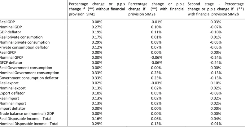
Table 17 - Simulation 2: effects on main macroeconomic variables ... 77
Table 18 - Simulation 2: aggregate results ... 77
Table 19 - Simulation 2: aggregate results. ... 78
Figure 14 - Simulation 2: aggregate results ... 78
Table 20- Effects on disposable income (percentage changes) ... 78
Figure 15 - Labour market dynamics ... 83
Table 21 -Financing source with transfer cut ... 93
Table 22 -Financing source with PIT increase... 93
Table 23 –Effects on employments of the intervention ... 94
Table 24- Changes of marginal PIT tax rates ... 94
Table 25- Changes in labour supply after the CGE shocks ... 95
Table 26- Percent changes in macroeconomic variables in simulations. ... 96
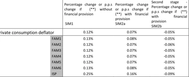
Table 27- Percent changes in real household consumptions in simulations... 96
Table 28- Percent changes in deflators of household consumptions in simulations. ... 97
4
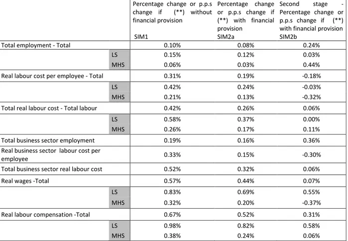
Table 30- Percent changes in labour market variables in simulations. ... 98
Table 31 - Content in skill of commodities ... 114
Figure 16 - Percentage changes in simulation vs. benchmark trend for LS, MS and HS workers. ... 116
Table 32 – Percentage changes in macroeconomic variables in simulations ... 118
Table 33 - Percentage changes in real consumption by household type and NPISH in simulations... 119
Table 34 - Percentage changes in the deflator of private consumption by household type and NPISH in simulations. ... 120
Table 35 - Percentage changes in employment and labour-cost variables in simulations. ... 120
Figure 17- Percentage changes in employment by skill in LS simulation. ... 121
Figure 18 - Percentage changes in employment by skill in HS simulation. ... 121
Figure 19 - Percentage changes in the real labour cost per employee by skill in LS simulation. ... 122
Figure 20 - Percentage changes in the real labour cost per employee by skill in MHS simulation. ... 122
Figure 21 - Percentage changes in real wages by skill in LS simulation. ... 123
Figure 22 - Percentage changes in real wages by skill in HS simulation. ... 123
Table 36 – Percentage changes in employment by labour category in LS simulation. ... 123
Table 37- Percentage changes in employment by labour category in HS simulation. ... 124
Table 38 – Percentage changes in employment by labour group ... 125
Figure 23 - Changes in p.p.s in unemployment rates by labour group in LS simulation. ... 126
Figure 24 - Changes in p.p.s in unemployment rates by labour group in HS simulation. ... 127
Figure 25- Percentage changes in hour worked by activity in LS simulation. ... 128
Figure 26 - Percentage changes in hour worked by work category in LS simulation. ... 128
Figure 27- Percentage changes in hour worked by activity in HS simulation. ... 129
Figure 28 - Percentage changes in hour worked by work category in HS simulation. ... 129
Figure 29 - Percentage changes in employment by gender in LS- and HS simulations. ... 129
Figure 30 - Labour/capital elasticity estimation ... 132
Figure 31 - Labour elasticity estimation by skill ... 132
Table 12.1.1 - Distribution of labour compensation share by skill and activity ... 159
Figure 12.1.1 - Robustness check: percentage changes of RGDP and labour demand (in aggregated terms and by components) according to different values of substitution elasticity by skill (a-s) in the case of a consumption shock (Simulation 1) ... 160
Figure 12.1.2 - Robustness check: percentage changes of RGDP and labour demand (in aggregated terms and by components) according to different values of substitution elasticity by skill (a-s) in the case of an investment shock (Simulation 2) ... 162
Table 12.2.1 - Percentage distribution of labour compensation share by skill and activity ... 164
Table 12.3.1 - Classification of activities in ESA-2010 ... 165
Table 12.3.2 - Classification of labour by skill level in the SAM ... 166
Table 12.3.3 - Percentage changes in macroeconomic variables due to simulations. ... 166
Table 12.3.4 - Percentage changes in macroeconomic variables due to simulations. ... 167
Table 12.3.5 - Percentage changes in real consumption by household type and for NPISHs due to simulations. ... 168
Table 12.3.6 - Percentage changes in the deflator of private consumption by household type and for NPHOs due to simulations. ... 169
Table 12.3.7 – Percentage changes in the employment and labour costs due to simulations. ... 169
Table 12.3.8 - Percentage changes in employment by skill due to simulations. ... 170
Table 12.3.9 – Percentage changes in the real labour-cost per employee by skill due to simulations. ... 170
5
General summary
Starting from the second half of 1990s, economic systems have deeply changed both because of the intensifying globalisation and of the massive introduction of digital innovation, as well as of progressive automation. These trends have affected the labour demand composition by skills (OECD, 2010). While the demand for low-skilled (LS) labour shrank (lowering LS wages), high-skilled (HS) labour demand more than offset the increase in HS labour supply by causing the increase in their wages (Oesch, 2010). Empirical evidences seem to confirm the complementarity between HS labour demand and capital, and a substitutability between LS labour demand and capital; however, the determinants of low-skilled unemployment reduction should be investigated at national and sectoral level.
In this framework, the evaluation of digital skills in the labour market is assuming a strategic role. Furthermore, a higher incidence of HS working force - in association with the adoption of ICT technologies - appears to be strongly correlated with a robust, sustainable and equal growth patterns. A particularly relevant aspect of the analysis of this problem consists in the use of Computable General Equilibrium (CGE) models, in order to study the general equilibrium consequences of ICT development.
In this context, as for the Part 1, a Social Accounting Matrix (SAM) of the Italian economy for 2013 has been built in order to study labour demand pattern changes. 12 labour components (the considered dimensions are the following: 3 types of occupations, 3 formal educational attainment levels and 2 levels of digital competences related to “computer use/not use” according to the PIAAC definition conveniently modified, in order to stress the aspect related to a complex use of computers and programming) have been distinguished. Based on the SAM, the Chapter 6 updates the MAC18-CGE Model developed by the Department of Economics and Law of the University of Macerata for 2011.
The Chapter 6 evaluates how fiscal policies affect the composition of employment by skill and occupation through changes in prices and quantities. The Chapter defines which measures can contribute to increase the share of the most skilled labour components with a higher digital competence on the total labour demand. In particular, the Chapter investigates the effects of a sectoral policy targeted to support HS digitalised work through a change in the composition of households’ private consumption as well as in the composition of investment.
The final demand policy is a way to stimulate the change in productive systems towards more knowledge-intensive products. This policy should be accompanied however by a policy aimed at supporting the change in labour supply through Vocational Education Training (VET) and Life-Long Learning (LLL) programmes.
The CGE model will contribute to find a comprehensive and coherent solution to evaluate the labour demand changes through the disaggregation by activity and the possibility of distinguishing the different labour components. Results seem to confirm the effectiveness of final demand
6 policies in order to support knowledge-intensive activities, especially in the case of a change in the composition of workforce.
Further results can be obtained by integrating the macro dimension of the SAM - which the CGE models is built on - with the micro dimension of a Tax and Benefit (TB) microsimulation model. In this context, the second part uses the same MAC-18 CGE model, but the aspect of non-perfect competition and of the involuntary unemployment in the labour market is stressed. Furthermore, we have considered the year 2014 and have decomposed the labour input into 24 components (by gender also). Furthermore, the gender gap is addressed, in order to take into account the different behaviour of labour supply by gender. The macro CGE model is integrated with the a microsimulation module allowing accounting households’ behaviour, which is differentiated according to the personal income tax breaks currently applied in Italy. The CGE model evaluates how the macroeconomic sectoral shock reverberates on the labour demand and ahead on the employment level. Then, the micro-simulation module shows how the changes in macroeconomic variables affect households’ behaviours in terms of labour supply and consumption demand.
The Chapter 8 of the thesis also evaluates the effects of a 1-p.-p. cut in SSC rate by using a dynamic CGE model, where capital and labour supply are endogenous. In particular, labour supply changes both through the population ageing, and the effectiveness of LLL and VET programmes in terms of skill developments. The transition from a static to a dynamic approach implies to consider cuts in SSC rates not only as a short term support for the weak component of the labour market, but as a possibility of maintaining or increasing the know-how owned by the weak component through the learning-by-doing mechanism.
Training programmes carried out by employers could be useful to increase workers’ human capital, even though there could be some negative effects (the locking-in effect, the low impact on short term and the substitution effect between trained and not-trained). Results of the simulations generally show small effects at the aggregated level. Real investment plays an important role, especially with the ICT innovation. This latter (in the absence of an increase in the aggregate demand) exerts a negative effects on total employment. However, high-skilled workers seem to be less damaged than low-skilled ones.
Finally, there is an estimation exercise of labour/capital substitution elasticities through an econometric approach by using systems of simultaneous equation. This exercise represents a useful integration of general equilibrium analysis, as substitution elasticities represents strategic parameters for CGE results. This is particularly true in the case of the decomposition of labour in several components.
7
1 - Introduction
Advanced countries have been hit over the last thirty years by a radical change in the economic paradigm, which has affected employment both in terms of level, and of composition. We can list the main drivers of these changes as follows: 1) globalisation and 2) digital innovation and progressive automation.
As for the globalisation, new (and often relevant) countries begun to be integrated in the world’s trade flows. In this context, changes in the labour geography (also seen as the Global Value Chains - GVCs) occurred. Moreover, low value added productive phases have been transferred towards countries with a relatively higher amount of (often unskilled) labour. Conversely, high-value added productive phases moved towards countries with a relatively higher amount of capital and skilled work. In this context, Italy is specialised in traditional and low technology productions and its endowment of skilled work is relatively lower than in similar countries.
The second mega-trend is represented by a pervasive ICT innovation both in services, and in manufacturing. In this context, the increase in supply of high-skilled workers is associated with a higher productivity - or GDP growth pattern of the skill-biased technological change (SBTC). The SBTC is a long-term trend and the introduction of digital technologies and of ICT innovations could allow to register its effects. This allowed a progressive automation of production phases, by determining an increase in productivity levels with a consequently higher GDP growth rate.
However, the distribution of advantages has been homogenously distributed neither around the world nor within country’s labour markets with increasing job opportunities and higher wages for HS workers, decreasing job opportunities for middle-skilled (MS) workers (with complete loss of labour compensation) and decreasing wages for elementary occupations and sales jobs (whose labour demand has generally maintained the existing levels). In terms of composition of the output, in advanced countries, the share of high-knowledge-intensive services (KISs)) and high-technology manufacturing (HTM) has increased with a reduction in low-knowledge-intensive services (LKISs) and low-technology manufacturing (LTM). In some other countries (especially the European Mediterranean ones) the (even if declining) building sector, as well LKISs have increased their share. At this regard, one has to underline the progressive ageing process, which has been increasing the demand for home assistance and household services.
The SBTC has increased the aggregate level of productivity both via the increased share of ICT-producer activities, and via the increased pervasiveness of ICT investments in all the economic activities. A higher weight of ICT-producing activities or a higher intensity of ICT investments is associated with enhancements in productivity patterns (see Bresnahan et al., 2002). ICT innovation requires an adequate composition of workers’ labour supply in terms of skill to unlock its whole effects. Indeed, the positive impact of skills on productivity is achieved only if the increased skilled labour supply matches with the higher demand for skilled work. At this regard,
8 according to OECD, 2003, skills and ICT seem to be complementary with higher wages associated with higher ICT investment. Bartelsman and Doms, 2000 and Doms et. al., 1997 use microdata to assess the existence of a positive relation between the number of advanced technologies used and workers’ skills (i.e. above-average skilled workers are probably better able to adopt the latest technologies).
The definition of (digital) skills has been developed in EC, 2016 and OECD, 2016. As for EC definition, components of digital competence is articulated in 5 areas which can be summarised as follows: i) information and data literacy; ii) communication and collaboration; iii) digital content creation; iv) safety; v) problem solving. The distribution of digital competences among workers is not homogeneous with different patterns by age classes. Highly digitally integrated environments allow also improvements in information management, protection and development to resolve conceptual problems. Skill endowment constitutes a relevant factor driving the distribution of advantages of GDP increase due to innovation (Matzat and Sadowski, 2012).
An operational tool to evaluate the level and the diffusion of abilities and skills across the economic systems is given by the survey on the Programme for the International Assessment of Adult Competences (PIAAC) by OECD. OECD, 2013 and 2016 synthesised the results of the PIAAC survey, which identifies three main cognitive skills (that is, literacy, numeracy and problem solving in technology-rich environment). The survey investigates the socio-demographic characteristics linked to skill proficiency (i.e. the educational attainment), as well as the way and the measure how the owned skills are used in the workplace and the way how skills are developed, maintained and/or lost.
ICT seems to have had positively contributed to economic growth and productivity dynamics (OECD, 2003 OECD 2016 and OECD Ministerial Meeting declaration1), even though benefits are not homogenously distributed among countries with some countries gaining a higher growth (the US, Canada, the Netherlands and Australia), and some others with lower benefits (France and Italy). More specifically, this can be due to the following factors: a) direct costs of ICT; b) costs and implementation barriers related to enabling factors (know-how or qualified personnel); c) risks and uncertainty (administrative burden); d) productive structure (i.e. not all activities benefit in the same way from ICT); e) competition.
ICT seems to favour countries with a more qualified labour endowment, so that increase in Life-Long-Learning (LLL) programmes could be a possible solution (Leahy and Wilson, 2014). The gap between advanced and laggard countries is also registered through the World Economic Forum (WEF) index2 (WEF, 2017). Indeed, WEF, 2017 shows that Mediterranean countries have
1 In 2016 Ministerial Meeting declared OECD, that in the framework of digitalisation “the digital economy is a powerful
catalyst for innovation, growth and social prosperity; that our shared vision is to promote a more sustainable and inclusive growth focused on well-being and equality of opportunities, where people are empowered with education, skills and values, and enjoy trust and confidence”. http://www.oecd.org/internet/ministerial/
2
This index is the result of four sub-indices measuring the formal educational attainment and cognitive skills (i.e. capacity), the skills acquired by employed (i.e. deployment), the increase in skills achievable through further formal
9 performed below the global average due to a higher rate of (youth) under-employment and unemployment rate. Moreover, these countries show a low labour market participation, a marked segmentation of labour market damaging women and young people, as well as a low quality of up- and re-skilling programmes.
The Chapter 5 contains a survey of the literature about modelling of labour market in CGE models. The paragraph 6.1 reports a survey of the literature about the megatrends of the labour market, confirming that skill developments and economic growth are strictly interwoven. Moreover, it contains a review of policies adopted by many countries to address the challenges of the ICT innovation. In this way, a robust and sustainable economic growth can be achieved only through an increase in the share of skilled work. A particular attention is paid for the value of elasticity coefficient of the labour demand by skill (see Chapter 8). The tool adopted to address this issue is the estimation of the Social Accounting Matrix (SAM) for the Italian Economy in 2013 (see Chapter 2). The SAM developed in the paper is relative to Italy in 2013; moreover labour is disaggregated into occupations and formal/digital skills, where these latter are obtained with answers about the use of computer, internet and simple/advanced programmes at work, as turning out from PIAAC database.
On the base of this SAM the products with the highest content of ICT skills, as well as high-qualified workers, are identified (see Paragraph 6.3). The SAM is also used to update and modify the MAC18 Computable General Equilibrium (CGE) model developed by the Department of Economics and Law of the University of Macerata (see Chapter 3). The model allows representing the relations between the changes in output of activities and the changes of compensation of employees by skill, digitalisation degree and gender in the context of the general equilibrium relations where both prices and quantities can adjust. Paragraph 6.4 will finally report results of the CGE simulations.
The next evolution step of the analysis is given by the integration of the microsimulation model with the macro sector CGE model through a convenient linking procedure (see Chapter 4). The Paragraph 7.2 analyses the literature on Micro-Macro integration. The Paragraph 7.3 addresses the issue of employment subsidies. Results of employment subsidies are summarised in the Paragraph 7.4.
The final part of the document is devoted to the estimation of labour/capital substitution elasticities, as well of elasticities among labour components (Paragraph 8.2) after a detailed literature review (Paragraph 8.1).
education for young people and upskilling/reskilling programmes for adult population (i.e. development), and the breadth and depth of specialised skills use at work (i.e. the know-how)
10
2 – The Social Accounting Matrix for skill analysis. Data description.
2.1 - The Social Accounting Matrix for skill analysis.
The Social Accounting Matrix (SAM) represents a useful and efficient tool to analyse the impact of a macroeconomic shock on labour compensation decomposed by formal education attainment, digital skills and gender among industries. Sir Richard Stone elaborated the first SAM in 1960 as the representation of transactions in a socio-economic system (Round, 2003) in relation with the Cambridge Growth Project. Since 1960s, the latter aspects emerged, also thanks to the ILO World Employment Programme (ILO, 1970) in 1970s. Models that are more complete were built in1970s with Iran, Sri Lanka and Swaziland (ILO, 1971, 1973, 1973b and 1976).
The SAM describes all the phases of circular flow of income from its generation in the production process (total output and value added generation), through its allocation in the distributive process (value added by factor, and primary and secondary income distribution) to the use of the disposable income in terms of final demand (Stone, 1985).
The SAM used in this paper is represented in Table 1. The market clearing condition for goods can be described as follows by taking into account both the first row and column:
∑mj=1Mj,i+ ∑CTct=1Tct,i+ ∑RTMrtm=1mrtm,i+ ∑ROWrow=1Irow,i=
∑m Zi,j
j=1 + ∑Ss=1Ci,s+ ∑row=1ROW Ei,row+∑INVinv=1Ii,inv (EQ1),
where the supply of (domestic Mj,i and imported Irow,i) goods including product taxes Tct,i and margins mrtm,i equals the intermediate consumption Zi,j and the final demand, as sum of the final
consumption Ci,s, exports Ei,row and investments Ii,inv.
The second constraint is that the value of production is equal to the sum of cost for intermediate consumption, primary factors and for taxes on activity output:
∑ni=1Mj,i= ∑ni=1Zi,j+ ∑Ll=1LCl,j+ CR.,j+ ∑ACTact=1Tact,j (EQ2),
where the value of output carried out by each activity Mj,i is given by the sum of the intermediate
consumption Zi,j, the cost of primary factors (labour LCl,j and capital CR.,j), as well by revenue of production taxes Tot,j (among them there is the tax on productive activity IRAP levied on the remuneration of primary factors).
The third constraint is that the demand for primary factors is equal to the supply of them plus the net inflow from abroad:
∑m LCl,j
11 where the labour and capital demand (respectively, LCl,j and CR.,j ) is equal to the supply by
national institutional sectors (respectively, LCsi,l and CRsi,.) and the rest of the world (ΔLCrow,l and ΔCRrow,.). The fourth constraint is given by the equivalence of output taxes levied on activities Tot,j
and the taxes received by the institutional sectors (taxes received by national sectors Tsi,ot and by the rest of the world ΔTrow,ot):
∑𝑚𝑗=1𝑇𝑜𝑡,𝑗 = ∑𝑆𝐼𝑠𝑖=1𝑇𝑠𝑖,𝑜𝑡+ ∑𝑅𝑂𝑊𝑟𝑜𝑤=1𝛥𝑇𝑟𝑜𝑤,𝑜𝑡 (EQ4).
At the same way we can reconstruct the constraint for commodity taxes:
∑𝑛 𝑇𝑐𝑡,𝑖
𝑖=1 = ∑𝑆𝐼𝑠𝑖=1𝑇𝑠𝑖,𝑐𝑡+ ∑𝑅𝑂𝑊𝑟𝑜𝑤=1𝛥𝑇𝑟𝑜𝑤,𝑐𝑡 (EQ5).
The next equation is the budget constraint of institutional sectors, where the received income YDsi,., in terms of both net income and tax revenues Revsi,., should equal the use of income for final consumption Ci,si and savings Sinv,si:
YDsi,.= ∑L LCsi,l
l=1 + CRsi,.+ ∑SIsǐ =1TRsi,sǐ + ∑ROWrow=1ΔTRsi,row− ∑ITit=1Tit,si(EQ6’),
Revsi,.= ∑OT Tsi,ot
ot=1 + ∑CTct=1Tsi,ct+ ∑ITit=1Tsi,it(EQ6’’),
YDsi,.+ Revsi,.= ∑ni=1Ci,si+ ∑INVinv=1Sinv,si (EQ6’’’).
The seventh constraint is given by the equivalence of income taxes paid by institutional sectors and the income taxes received by the institutional sectors:
∑SI Tit,si
si=1 = ∑SIsi=1Tit,si (EQ7).
The eighth constraint is that the sum of trade and transport margins mrtm,j by activity is zero:
∑mj=1mrtm,j= 0 (EQ8).
The last two constraints are about the budget constraint for the rest of the world with the import and the net inflows for primary factors, taxes and transfers as received income and export and the opposite of the current account as income usages:
∑ni=1Irow,i+ ∑Ll=1ΔLCrow,l+ ΔCRrow,.+ ∑ot=1OT ΔTrow,ot+ ∑CTct=1ΔTrow,ct+ ∑SIsi=1ΔTRsi,row =
∑ Ei,row+ ∑INV Sinv,row
inv=1 n
i=1 (EQ9).
The last constraint is the equivalence of the sum of savings and the investment flows:
∑SI Sinv,si
12
Table 1 - The structure of the SAM
Source: Authors’ elaboration.
com1…..i…….n act1…...j…..m L1…..l……L K Out_Tax1…..ot……OTCom_Tax1…..ct……CT Inst_Sect1….s….S Inc_Tax1….it….IT RTM1…....rtm…..RTM ROW INV1…..inv…..INV Row total
com1…..i…….n Intermediate consumption [Zi,j] Final consumption [Ci,s] Export [Ei,row] Investments [Ii,inv] q 1….q i……q n act1…...j…..m Make Matrix [Mj,i] x 1….x j……x m L1…..l……L K Out_Tax1…..ot……OT Output taxes paid [Tot,j] Output taxes paid [Tot,row] OT 1…O T ot …O T OT Com_Tax1…..ct……CT Commodity taxes paid [Tct,i] Commodity taxes paid[Tct,row] CT 1…C T ct …C T CT Inst_Sect1….s….S Output taxes received [Ts,ot] Commodity taxes received [Ts,ct] Secondary transfers [Trs,s] Income taxes received [Ts,it] Secondary transfers [Trs,row] Y 1…… .… ...Y s… …... ..…Y S Inc_Tax1….it….IT Income taxes paid [Tit,s] IT 1..…It it..… IT IT RTM1…....rtm…..RTM Retail and transport margins [mrtm,i] 0… …… …..0 …… ...0 ROW Import [I.,i] Output taxes [Trow,ot] Commodity taxes [T row,ct] Secondary transfers [Trow,s] Y RO W
INV1…..inv…..INV Savings [Sinv,s]
Savings [S inv,row] IN V 1…IN V inv….IN V INV
Colmun total q1….qi……qn x1….xj……xm OT1…OTot…OTOT CT1…CTct…CTCT Y1…...Ys...…YS IT1..…Itit..…ITIT 0…………..0……...0 YROW INV1…INVinv….INVINV Labour compensation [LCrow,l] + capital remuneration [CRrow,.] LC1…LCl….LCL KR LC 1…..L C… …… …..L C L KR Labour compensation [LCsi,l] + capital remuneration [CRsi,.] Labour compensation [LCl,row] + Capital remuneration [KR.,row] Labour compensation [LCl,j] + Capital remuneration [CR.,j]
13 In the framework described by the previous equations, the SAM could be defined as a comprehensive and coherent representation of the flows of the economy from the income generation, through the allocation of primary income to institutional sectors and the secondary distribution flows, until the final expenditures for consumption and savings (Miller and Blair, 2009). These relations can be used to construct the CGE model by the introduction of prices that in the benchmark are supposed to be equal to the unit.
2.2 – Macro data description
The main data-source of the SAM is the National Accounting Matrix (NAM). In the first paper we have used the matrix relative to 2013 (ISTAT, 20163), differently from the second paper where the 2014 edition has been used ISTAT, 20194).
It provides a general scheme to elaborate the income generation divided in 20 activities and attributes primary incomes by 3 income types (labour compensation, gross operating surplus and mixed income) and 6 institutional sectors (financial and non-financial corporation, public administration, consumer- and producer households and social private institutions). The database provides additional information about the formation and the use of the disposable income.
These data are elaborated using the Input-Output table at purchaser’s price with 63 activities for 2013 released by ISTAT, 2016b5 in the first paper and for 2014 released by ISTAT, 2019b6 in the second paper. The labour compensation has been disaggregated in the first paper into 12 classes by occupation, educational attainment and ICT skill deriving from PIAAC data. In the second paper, we have added the gender dimension by obtaining 24 components.
The disaggregation of the ‘Compensation of employees’ component is made in relation to gender, formal qualification and digital competences. In detail, we have three groups of skills: i) no formal qualification up to the primary school diploma, ii) high school diploma; and iii) university degree (from PIAAC database). Digital competences are divided into ‘workers with skills - Skill’ (‘computer use’) and ‘No skill - Unskill’ (‘computer no use’). This latter index is obtained as the weighted average of the use of e-mail (5 per cent), the use of internet to better understand questions related to work (7 per cent), e-commerce and e-government (10 per cent), the use of excel (13.5 per cent), the use of word (17.5 per cent), the use of complex programming (22 per cent) and the use of video-conference and other real-time participation to discussion (25 per cent). For this disaggregation, we have used the data from PIAAC database integrated by EU-SILC.
In particular, occupations are distinguished among high-skilled, medium skilled and low skilled; formal educational attainment is classified between low-educated, medium educated and tertiary educated. Digital competences have been assessed by using PIAAC answers about the use of computers, e-mail and simple/advanced programmes at work. The Table 2 gives a detailed 3 See https://www.istat.it/it/archivio/196839 . 4 See https://www.istat.it/it/archivio/209141 . 5 See https://www.istat.it/it/archivio/208938 . 6 See https://www.istat.it/it/archivio/225665.
14 description of the labour components. The first level of aggregation is represented by gender with components 1-12 are related to the male components and 13-24 to the female one.
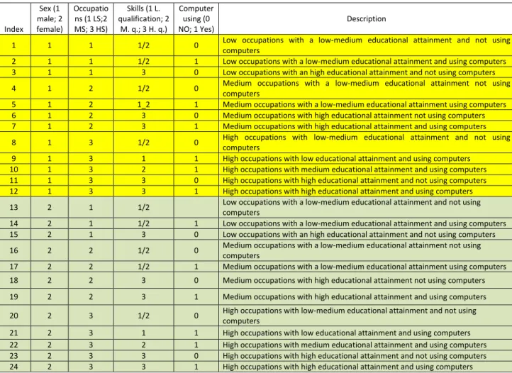
Table 2 - Classification of labour factor in the SAM
Index Sex (1 male; 2 female) Occupatio ns (1 LS;2 MS; 3 HS) Skills (1 L. qualification; 2 M. q.; 3 H. q.) Computer using (0 NO; 1 Yes) Description
1 1 1 1/2 0 Low occupations with a low-medium educational attainment and not using computers
2 1 1 1/2 1 Low occupations with a low-medium educational attainment and using computers 3 1 1 3 0 Low occupations with an high educational attainment and not using computers 4 1 2 1/2 0 Medium occupations with a low-medium educational attainment not using
computers
5 1 2 1_2 1 Medium occupations with a low-medium educational attainment using computers 6 1 2 3 0 Medium occupations with high educational attainment not using computers 7 1 2 3 1 Medium occupations with high educational attainment and using computers 8 1 3 1/2 0 High occupations with low-medium educational attainment and not using
computers
9 1 3 1 1 High occupations with low educational attainment and using computers 10 1 3 2 1 High occupations with medium educational attainment and using computers 11 1 3 3 0 High occupations with high educational attainment and not using computers 12 1 3 3 1 High occupations with high educational attainment and using computers 13 2 1 1/2 Low occupations with a low-medium educational attainment and not using
computers
14 2 1 1/2 1 Low occupations with a low-medium educational attainment and using computers 15 2 1 3 0 Low occupations with an high educational attainment and not using computers 16 2 2 1/2 0 Medium occupations with a low-medium educational attainment not using
computers
17 2 2 1/2 1 Medium occupations with a low-medium educational attainment using computers 18 2 2 3 0 Medium occupations with high educational attainment not using computers 19 2 2 3 1 Medium occupations with high educational attainment and using computers 20 2 3 1/2 0 High occupations with low-medium educational attainment and not using
computers
21 2 3 1 1 High occupations with low educational attainment and using computers 22 2 3 2 1 High occupations with medium educational attainment and using computers 23 2 3 3 0 High occupations with high educational attainment and not using computers 24 2 3 3 1 High occupations with high educational attainment and using computers
Source: Own elaborations
A the second level, the leading criterion is given by occupations with components 1-3 for males and 13-15 for females concerning LS occupations, 4-7 and 16-19, respectively for both genders, for HS occupations, as well as 8-12 and 20-24, respectively, for HS occupations. The third level of aggregation allows us to conduct an in-depth analysis of the relationship between formal skills requested by occupations and those owned by workers. More precisely, the components 1-2 and 13-14 could be considered as the occupation/worker combinations characterised by a substantial matching for low skills. The same occurs for medium skills in components 4-5 and 16-17. Moreover, components 11-12 and 23-24 register the condition of perfect matching for high skills. Overkilling (i.e. the condition of workers owning higher skills than those requested by occupations) can be found in components 3 and 15, where HS workers perform LS tasks. The situation is only slightly more favourable in components 6-7 and 18-19, where HS workers performs MS tasks. Undereducation (i.e. the condition of workers owning lower skills than those requested) seems particularly severe in components 9 and 21, where LS workers perform HS occupations. The phenomenon seems less severe in components 8 and 10, and 20
15 and 22, where MS workers are employed in HS occupations. The fourth dimension is represented by ICT informal skills and offers a hint for the adoption of digital innovation by firms. Components 9, 10 and 12, as well as 21, 23 and 24 include HS occupations using ICT competences and this is particularly relevant for the components 9-10 and 21-22, where MLS workers perform HS occupations. ICT competences are also used in components 5 ant 7, and 17 and 19 for MS skills, as well as 2 and 14 for LS workers.
The primary distribution to institutional sectors has been made by using the original classification of the NAM 2013 and 2014, aggregating producer- and consumer-households, as well as disaggregating the public administration into six sub-sectors (central administration, social insurance bodies, regional, provincial, municipal and other local and central administrations).
A relevant feature in the SAM elaborated in the paper is that labour compensation includes only the gross wages - including employers’ SSCs - relative to dependent workers. In this way, independent work (including entrepreneurs, occasional workers, free-lance workers and members of workers’ owned companies) is not explicitly considered and its remuneration is included in the mixed income with other components (such as profits). Theoretically, this is not correct, because it determines an understatement of the effective labour input used in production (especially in countries with a high share of independent work). However, prices of independent work are more similar to profit or to remuneration of capital than to prices of dependent work which are determined through the wage bargaining. Therefore, summing-up the remuneration for independent work and capital could be suitable. A three-nested production function has been adopted. In the first nest, we have a Leontief production function aggregating intermediate consumption and the value added. Intermediate commodities are assumed to have fixed share intermediate consumption taken together, so by hypothesising also in this case a Leontief aggregation function. Primary factors capital and labour - which are part of the value added - are aggregated through a CES production function. In the same way, the aggregate labour input has been obtained from the aggregation of each specific labour type. Elasticities between capital and labour as well as among different types of labour have been defined on the base of the international literature.
The coefficient related to the capital/aggregated labour elasticity has been estimated on the base of OECD disaggregate data until 2009 and this could not take into account the consequences of the structural break of the economic crisis. In addition, the elasticity coefficient among labour types could be not suitable for the Italian 2013 condition, as it has been estimated on US data and for faraway periods.
We have to stress that the wage or the capital return rate calculated on the base of the National Account data can show a high heterogeneity degree across activities and this circumstance contradicts the assumption of a full mobility of production factors across activities/firms implied by the perfect competition. Wage- and return differentials could be modelled
16 as exogenous or endogenous. In our model, the production and the cost function are modelled based on the different types of labour compensation and capital remuneration, by hypothesising a factor price equal to one in the benchmark. This implies that in the benchmark wage- and return rate-differentials in terms of physical units of employment and capital are assumed to be different from zero and these differentials are endogenous, as they can change in simulations through factor prices higher/greater than 1.
Table 12.2.1 in Appendix shows the distribution of labour compensation by skill level of occupation and digital competence in 2014. We can see that generally the Italian productive system is characterised averagely by a use of computer and internet at work amounting to 37.5 per cent of labour compensation. About the 70 per cent of labour compensation paid to ICT skilled workers is paid to workers performing high-skilled occupations.
The more intensive activities of use of computers (see Tables 10.2.1 and 10.2.2 in the Appendix) are professional and scientific services (M74-75), programming activities (J62_63), legal and accounting services (M69_70) and insurance services (K65). Conversely, paper industries (C17), accommodation services (I), other personal services (S96) and household services (T) register a low level of ICT competences.
As for the institutional sector, two main changes have been introduced into the NAM 2014. First, the Public Administration sector has been divided into the following six sub-sectors: i) central administration; ii) pension- and social assistance institutions; iii) regional administrations; iv) province- and town-district7-level administrations; v) municipal administrations; vi) other administrations. Transfers between public administrations have been obtained by elaborating the data about the current transfers from the SIOPE database released by the Ministry of Economy and Finance and the Bank of Italy 8 and the Public Finance statistics from ISTAT9.
As for households, we have aggregated the NAM figures for consumer- and producer-households. Then, we have used the IT-SILC data integrated with the Consumer Survey (both released by ISTAT) and with the SHIW survey released by the Bank of Italy. Then the individual taxable income has been calculated and individuals have been classified according the five Personal Income Tax (PIT) brackets in force in Italy (<=15,000 with a gross rate of 23 per cent; 15,001-28,000 with 27 per cent; 28,001-55,000 with 38 per cent; 55,001-75,000 with 41 per cent; >75,000 with 43 per cent). Finally, households have been ranked according to the prevalence of components belonging to each PIT bracket (see households from FAM2-FAM6); a residual category (FAM1) has been identified for households without a precise identification.
As we can observe from the Table 3, the employment in low-skilled occupations is concentrated in the first two PIT brackets FAM2-FAM3 (52/53 per cent for males and 16/26 per cent for females without/with the use of computers at work). On the contrary, employment in
7
Town- districts include medium-large sized towns (such as Rome, Milan and Turin) with the same powers of provinces.
8
See https://www.siope.it/Siope/ .
9
17 skilled occupations is more concentrated (even though in a lesser extent) in the three richest PIT brackets (FAM4-FAM6) with a cumulated incidence of 21/31 per cent for males and 20/23 per cent for females (respectively, without and with the use of computers at work).
Table 3 - Allocation of the labour compensation by institutional sectors
Gender
Low-skilled occupations Medium-skilled occupations High-skilled
occupations Using computers
High skilled occupations Not using com. Using
com. Not using com.
Using com. Not using com. Using com. FAM1 Males 0.00 0.02 0.00 0.00 0.00 0.00 0.00 0.00 FAM2 13.04 16.20 9.35 7.33 4.46 6.04 6.94 5.47 FAM3 40.07 36.96 28.10 21.28 11.98 13.46 16.75 12.93 FAM4 16.11 27.81 11.50 16.32 13.41 24.36 22.57 20.43 FAM5 0.00 0.84 0.47 1.77 6.31 6.20 4.79 6.24 FAM6 0.74 0.33 0.35 0.73 1.49 8.22 5.91 5.81 ROW 0.20 0.24 0.14 0.14 0.11 0.17 0.17 0.15 FAM1 Females 0.00 0.00 0.00 0.00 0.00 0.00 0.00 0.00 FAM2 12.17 7.47 15.38 11.01 4.96 3.68 5.71 4.14 FAM3 14.02 7.63 24.76 25.78 20.66 14.56 16.93 16.74 FAM4 2.94 2.44 8.97 13.69 31.18 17.40 15.62 22.34 FAM5 0.51 0.00 0.60 1.01 2.72 2.70 2.13 2.71 FAM6 0.10 0.00 0.22 0.78 2.55 3.10 2.35 2.90 ROW 0.09 0.05 0.15 0.15 0.18 0.12 0.12 0.14 Total 100.00 100.00 100.00 100.00 100.00 100.00 100.00 100.00
Source: Authors’ calculation on ISTAT data (National Accounts) and PIAAC and EU-SILC data.
As we can observe from the Figure 1, male employment covers about 55 per cent of labour compensation at the aggregate level (see the dashed line). There is a high heterogeneity by activity with the male employment prevailing in Auxiliary activities to the financial sector (a43), Rental and leasing services (a50), Employment activities (a51), Repair of computers (a61), Repair and installation of machinery/equipment (a23), Water collection, treatment and supply (a25), Construction (a27), Forestry and logging (a2), Fishing (a3) and Manufacture of coke and refined petroleum (a10). Female workers are the majority in Households services (a63) and Other personal services (a62) with a relevant percentage in Education (a55) and in Human health (a56), Real estate services (a44), Legal and accounting activities (a45) and Air transport (a33).
Figure 1 - Allocation of the labour compensation by gender
Source: Authors’ calculation on ISTAT data (National Accounts) and PIAAC and EU-SILC data. 0% 20% 40% 60% 80% 100%
a1 a3 a5 a7 a9 a11 a13 a15 a17 a19 a21 a23 a25 a27 a29 a31 a33 a35 a37 a39 a41 a43 a45 a47 a49 a51 a53 a55 a57 a59 a61 a63
18 As for the labour compensation (see Figure 2), data confirm the existence of a gender gap amounting to 5.7 p.p.s normalised with respect to the average aggregate hourly labour compensation. We can observe an high heterogeneity among activities: the Manufacture of basic metals (a15) and of metal products (a16) register an high difference between male and female hourly wages, amounting respectively to 61 and 91 p.p.s.; in services there is a difference of 121.0 p.p,s favourable to male workers. Differences are negative and favourable to women in the Manufacture of wood and cork (a7 with -35.9) and of rubber and plastic (a13 with -37.3), as well as in the Rental and leasing activities (a50 with -53.9). In 31 out of 49 activities for which hourly wages are available both for both genders, there is a positive difference favourable for men.
Figure 2 - Average labour compensation per hour worked by gender (index with the aggregate
level=100)
Source: Authors’ calculation on ISTAT data (National Accounts) and PIAAC and EU-SILC data.
As for composition by skill (see Figure 3), averagely, LS work covers 22.9 per cent of labour compensation vs.36.5 of MS work and 40.6 per cent of HS work. LS work has a particularly high weight in Agriculture (a1 with 80.1 per cent), Forestry (a2 with 66.0 per cent), Sewage and waste management ( a26 with 66 per cent) and Land transport (a31 with 59.4 per cent). Instead, MS work is prevalent in Fishing (a3 with 59.6 per cent), Manufacture of woof and cork products (a7 with 69.9 per cent), Printing (a9 with 100 per cent), Vehicle trade (a28 with 73.0 per cent), Other retail trade (a30 with 79.4 per cent), Postal activities (a35 with 71.3), Accommodation (a36 with 81.6), Travel agency (a52 with 67.7 per cent) and Household services (a63 with 66.2 per cent). Moreover, the labour compensation of HS work is high in Real estate activities (a4 with 67.2 per cent),Manufacture of pharmaceuticals (a12 with 57.0), Electricity and gas (a24 with 53.0 per cent), Publishing activities (a37 with 63.0 per cent), Telecommunications (a39 with 70.6), Computer programming (a40 with 84.8), Financial services (a41 with 69.9), Insurance services (a42 with 70.3), Auxiliary financial services (a43 with 100.0), Architectural and engineering (a46 with 80.2),
0 50 100 150 200 250
a1 a3 a5 a7 a9 a11 a13 a15 a17 a19 a21 a23 a25 a27 a29 a31 a33 a35 a37 a39 a41 a43 a45 a47 a49 a51 a53 a55 a57 a59 a61 a63
19 Scientific research (a47 with 75.1), Other professional services (a49 with 68.8), Education (a55 with 80.6) and Human health (a56 with 75.0).
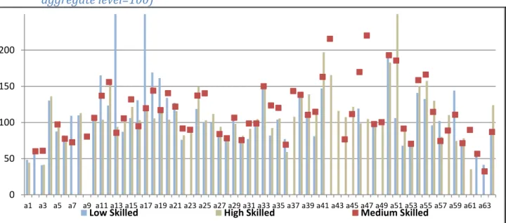
Figure 3 - Allocation of the labour compensation by formal skill
Source: Authors’ calculation on ISTAT data (National Accounts) and PIAAC and EU-SILC data.
Hourly labour compensations (see Figure 4) follows averagely the expected pattern in terms of values normalised to the average figure. Indeed, LS workers earn a wage equal to 90.5 per cent of the average value vs. 87.0 per cent of MS workers and 124.0 per cent of HS workers, even though no relevant difference emerges averagely between LS and MS work. In Manufacture of basic metals (a15), Manufacture of motor vehicles (a20), Rental and leasing activities (a50), Public Administration (a54) and Education (a55), all components earn an hourly wage higher than the average and MS work seems particularly favoured with a figure amounting respectively to 132.0, 140.5, 193.1, 158.6 and 166.3. In the both activities, HS workers are, respectively at 121.6, 103.9, 183.0, 150.5 and 157.7. Also, Manufacture of coke (a10), Manufacture of chemicals (a11) and Manufacture of pharmaceuticals (a12) generate wages higher than the average and the distribution of wages among components follows the expected pattern (LS wages<MS wages<HS wages) with the exception of a11, where LS workers are particularly favoured (165.3 vs. 137.1 and 103.9 for, respectively, LS and MS workers. Manufacture of electrical equipment (a18) and of machinery and equipment (a19) register an advantage for LS work with a figure amounting respectively to 169.3 and 161.4. MS workers’ wages is particularly high at 220.4 for a47.
As for the composition by skill (see Figure 5), averagely, perfectly matched work covers 73.0 per cent of labour compensation vs. 27.0 of not-perfectly matched work. 75.1 per cent of matched work is represented by LS work. Indeed, 16.9 per cent of unmatched work is constituted by overskilled work. The activities with the lowest incidence of the matched work are Auxiliary activities to financial services (a43 with 0.0 per cent), Scientific research (a47 with 25.4), Rental and leasing activities (a50) and Employment activities (a51) - both with 32.2 per cent - , Repair services (a61 with 47.3) and Electricity (a24 with 47.2). Computer programming (a40 with 29.8 per
0% 10% 20% 30% 40% 50% 60% 70% 80% 90% 100%
a1 a3 a5 a7 a9 a11 a13 a15 a17 a19 a21 a23 a25 a27 a29 a31 a33 a35 a37 a39 a41 a43 a45 a47 a49 a51 a53 a55 a57 a59 a61 a63
20 cent), Publishing activities (a37 with 37.4), Architectural and engineering (a46 with 33.7), Education (a55 with 26.3), Human health (a56 with 32.6) register particularly low figures for the incidence of LMS matched workers on matched workers. Indeed, the incidence of overskilled workers on unmatched workers is highest in Advertising (a48) and Household services (a63) - both at 100.0 per cent -, Accommodation services (a36 with 82.4), Travel agency (a52 with 55.0 per cent) and Air transport (a33 with 50.2).
Figure 4 - Average labour compensation per hour worked by formal skill (index with the
aggregate level=100)
Source: Authors’ calculation on ISTAT data (National Accounts) and PIAAC and EU-SILC data.
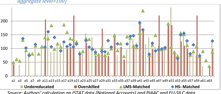
Figure 5 - Allocation of the labour compensation by match/mismatch
Source: Authors’ calculation on ISTAT data (National Accounts) and PIAAC and EU-SILC data.
As for the hourly labour compensation by skill (see Figure 6), averagely, perfectly LMS matched workers earn the 87.6 per cent of total economy wage and this represents the minimum. Overskilled workers earn 10.9 p.p.s more than LMS workers. Moreover, HS matched workers earn the maximum at 127.3 per cent of the average wage, followed by the undereducated ones (121.4).
0 50 100 150 200
a1 a3 a5 a7 a9 a11 a13 a15 a17 a19 a21 a23 a25 a27 a29 a31 a33 a35 a37 a39 a41 a43 a45 a47 a49 a51 a53 a55 a57 a59 a61 a63
Low Skilled High Skilled Medium Skilled
0% 10% 20% 30% 40% 50% 60% 70% 80% 90% 100%
a1 a3 a5 a7 a9 a11 a13 a15 a17 a19 a21 a23 a25 a27 a29 a31 a33 a35 a37 a39 a41 a43 a45 a47 a49 a51 a53 a55 a57 a59 a61 a63
21 The activities with the highest gross wage for all the four mentioned categories are the following: Manufacture of chemicals (a11), of pharmaceuticals (a12) and of motor vehicles (a20), Scientific research (a47) and Sport activities (a59) with particularly high values for overskilled workers; Manufacture of computers (a17), of electrical equipment (a18) and of machinery and equipment (a19), Insurance activities (a42) and Public Administration (a54) with particularly high wages for LMS matched workers; Land transport (a31), Water transport (a32), Warehousing (a34), Telecommunications (a39) with particularly high figures for HM matched workers; Electricity and gas (a24), Sewage and waste management (a26), Employment activities (a51), Education (a55) and Human health (a56), with particularly high values for undereducated workers. Financial services (a41), Legal and accounting services (a45), Other professional activities (a49), Rental and leasing activities (a50),Manufacture of other transport equipment (a21) and of paper products (a8) and Mining and quarrying (a4) register particularly high values without relevant differences among the mentioned components.
Figure 6 - Average labour compensation per hour worked by match/mismatch (index with the
aggregate level=100)
Source: Authors’ calculation on ISTAT data (National Accounts) and PIAAC and EU-SILC data.
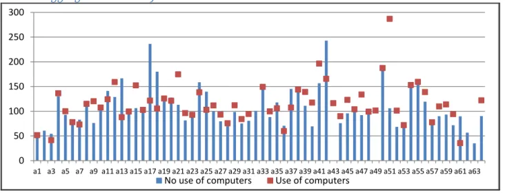
As for the composition by informal skills approximated by ICT competences (see Figure 7), averagely, averagely, ICT-intensive workers represent the 37.5 per cent of total labour compensation. There is a high heterogeneity among activities with particularly high figures in Other professional activities, rent and employment services (a4 to a52), Creative services (a58), Telecommunications and (also scientific) professional services (a3 to a47), Publishing (a37), Electricity and gas (a24), Manufacture of pharmaceuticals (a12) and Mining and quarrying (a4) with values higher than 60 per cent.
As for the hourly labour compensation by skill (see Figure 8), averagely, the hourly labour compensation of ICT-intensive workers amounts to 121.9 per cent of the total economy hourly gross wage index with a differential vs, non ICT-intensive workers amounting to 31.6 p.p.s. The
0 50 100 150 200
a1 a3 a5 a7 a9 a11 a13 a15 a17 a19 a21 a23 a25 a27 a29 a31 a33 a35 a37 a39 a41 a43 a45 a47 a49 a51 a53 a55 a57 a59 a61 a63
22 differential varies across activities and we can find activities with very low positive differentials or also negative ones.
Figure 7 - Allocation of the labour compensation by informal skills
Source: Authors’ calculation on ISTAT data (National Accounts) and PIAAC and EU-SILC data.
As for the first case we can list the following activities: Agriculture (a1), Mining and quarrying (a4), Manufacture of food and beverages (a5), of paper products (a8), of coke (a10), of other non-metallic mineral products (a14) and of furniture (a22), repair and installation services (a23), Sewage and waste management (a26), Construction (a27), Trade and land transport (a29 to a31), Warehousing (a34), Broadcasting programming (a38), Real estate activities (a44), Advertising (a48) and Security services (a53) and Public Administration and education (a54 and a55).
Figure 8 - Average labour compensation per hour worked by informal skill (index with the
aggregate level=100)
Source: Authors’ calculation on ISTAT data (National Accounts) and PIAAC and EU-SILC data.
Instead, as for the second group, the following activities can be listed: Fishing (a3),Manufacture of textiles (a6), of wood and cork products (a7), of chemicals (a11), of rubber and
0% 10% 20% 30% 40% 50% 60% 70% 80% 90% 100%
a1 a3 a5 a7 a9 a11 a13 a15 a17 a19 a21 a23 a25 a27 a29 a31 a33 a35 a37 a39 a41 a43 a45 a47 a49 a51 a53 a55 a57 a59 a61 a63
No use of computers Use of computers
0 50 100 150 200 250 300
a1 a3 a5 a7 a9 a11 a13 a15 a17 a19 a21 a23 a25 a27 a29 a31 a33 a35 a37 a39 a41 a43 a45 a47 a49 a51 a53 a55 a57 a59 a61 a63
23 plastic (a13), of metal, computer and machinery (a16 to a20), Electricity and gas (a24), Water collection (a25), Trade of motor vehicles (a28), Air Transport (a33), Postal, publishing and accommodation services (a35 to a37), Insurance (a42),Architectural and engineering (a46), Employment services (a50) and Repair of computers (a61).
2.3 - Description of microeconomic data
The IT_SILC database contains information about income, as well households. Incomes are reported as net of taxes, so that they should made gross by summing up direct taxes (distinguishing by the beneficiary administration) and subtracting benefits (such as tax deductions from taxes or taxable income). This allows obtaining the disposable income, whose sum has to be equal with national accounts. The use of income and wealth is obtained by linking IT_SILC with SHIW and microdata from consumer survey through an imputation technique, so to obtain the household’s consumer propensity and an aggregate one, which should be consistent with microdata. Changes in disposable income determine changes in individual labour supply in terms of hours.
Our microeconomic dataset is based on the 2014 IT-SILC data with income data related to 2014 and labour market statuses related to 2013. The base has then been enriched through matching procedures with the 2014 SHIW survey and the 2013 Consumer survey. This approach allows combining the statistical representativeness of SILC data with the particular attention paid by SHIW to the wealth (even though these data are not representative at regional level and upward biased) and with the detail by COICOP assured by the Consumer Survey.
With particular reference to the disaggregation of consumption by commodity, we have estimated the weights transforming COICOP into the NACE classification through an equation system through a Seemingly Unrelated Regression (SUR) model. This step is very useful, as it allows us to estimate the change in households’ consumption patterns after a change at the microeconomic level, originated either from the micro level itself, or as a response to a macroeconomic shock.
Our micro dataset contains 47,136 observations, representing 60,623,518 people. The dataset includes the gross employees’ income with a poor and reliable detail by activity, but a rich detail in terms of time (hours/months) worked, type of contract and reasons to work/not work. This allows us to extract from inactive people’s pool the potential labour force (PLF) including inactive people not searching for a job, but still available to work. From the dataset we can also obtain reliable (even though not complete) estimation of jobs which people and especially unemployed and PLF inactive are searching for. By combining information about the hour worked, the reasons to work/not work and job expectations, we are able to determine the potential employment and income. The potential employment and income differ from the actual ones because of the amount attributed to involuntary part-time or fixed-term workers, unemployed and PLF members. We can
24 describe all these quantities as an activation margin in case of a positive shock on employment at the macro level.
Labour Force Survey (LFS) micro data provide for a decomposition of population by occupational statuses (employed, unemployed and inactive) and allow analysing detailed aspects of each individual’s life, such as gender, age, education, residence and other drivers of choice of individuals. Since 2011, LFS data contain data on wages too. LFS data also allow analysing the emerging skill mismatch if there is match between the formal skills requested to perform a task and those owned by the workers. EUKLEMS provides for a survey report on gender, gender and skills by economic sectors until 2014. Not-formal skills are not available in LFS data. At this regard, we can found information by opportunely combining data on innovation by firms with data on formal education by sectors.
25
3 - Macro sectoral CGE model description.
3.1 - Description of the static CGE model.
The model used in all the papers is the MAC-18 model od Computable General Equilibrium (CGE), developed by the Department of Economics and Law of the University of Macerata. The main target of the model is to quantify the economic, disaggregate, direct and indirect impacts of fiscal policies and policy reforms on the Italian macroeconomic variables. The main assumption of the CGE models is that there is perfect competition in all markets, so that the constrained maximising choices of households, firms, public administrations and private social institutions determine simultaneously prices and quantities according to policy changes in final demand or in other parameters. In order to make the model more coherent with the actual situation, a wage curve scheme explains wages. The relations among prices and quantities are summarised in Table 4, which is similar to the Table 1, but it distinguishes the endogenous and exogenous variables.
By recalling the EQ1 defined in the explanation of the SAM, the supply of goods Qi has offered both by domestic firms producing according to a CES production function Xj and by the rest of the world through imports. These latter depend on prices of output by activity paj, revenues of taxes on output function of the rate of taxes on output toi, as well of import function of import prices pmwi.. The demand of goods comes from the following sources: i) the intermediate consumption from activities depending on the volume of output Xj (hypothesis of a Leontief production function with fixed shares); ii) final demand for households’ consumption depending on pi and the disposable income of households Yh; iii) the final demand public administration assumed fixed at Gg; iv) investment I according to the price of each good pi and the aggregate level of saving S; as well as v) the rest of world depending on the competitiveness given by pi∙EXR/PROW (where EXR is the exchange rate and PROW is the price on international markets under the assumption of exporters being price-takers).
As for the EQ2, the price of output by activity paj is defined as a cost function with two nests modelled as a Leontief function as for the aggregation of intermediate goods B(Xj,pi) and of primary factors VA(Xj,pvaj). These latter are modelled as a CES function in the labour compensation and in capital remuneration. In the original version of the model there is only one type of labour compensation, whereas in the revised version the labour compensation is a CES aggregation of 12 (or 24) different types of labour compensation, disaggregated by (gender), occupation, educational attainment and digital competence.
As for the EQ3, the value added generated by activity j VAj is attributed to domestic private institutional sectors h as gross market income Yfh, to the different levels of public administration (Yfg), as well to the rest of world (YfROW). The labour compensation is attributed to households and to the rest of the world, whereas the gross operating surplus (including also mixed income potentially earned by independent workers) is divided among all domestic and foreign institutional sectors.
26
Table 4– The structure of the MACGEM-IT model
Source: Authors’ elaboration.
com1…..i…….n act1…...j…..m L1…..l……L K Out_Tax1…..ot……OTCom_Tax1…..ct……CT Inst_Sect1….s….S Inc_Tax1….it….IT RTM1…....rtm…..RTM ROW INV1…..inv…..INV Row total
com1…..i…….n B(Xj,Pi)
C(Yh,pi)
and Gg
E(Pi,EXR,PROW) I(S,pi)
q 1….q i……q n act1…...j…..m bi(Qi, paj) x 1….x j……x m L1…..l……L K
Out_Tax1…..ot……OT Ta(Xj, taj)
OT 1…O T ot …O T OT
Com_Tax1…..ct……CT To(Qi,toi)
CT 1…C T ct …C T CT
Inst_Sect1….s….S Ta(Xj, taj) To(Qi, toi)
Tr(Yfh,trtrash) and Tr(Yfg, tr tras g) Ty(yfh, ty inc h) TrROW Y 1…… .… ...Y s… …... ..…Y S
Inc_Tax1….it….IT Ty(Yfh, tyinch)
IT 1..…It it..… IT IT RTM1…....rtm…..RTM 0… …… …..0 …… ...0 ROW M(Qi, Pmi , pwmi)
Tr(Yfh,trtrasROW)
and TrgROW Y RO W INV1…..inv…..INV S(Yfh,r) and S(Yfg,r) (+/-)SROW IN V 1…IN V inv….IN V IN V
Colmun total q1….qi……qn x1….xj……xm LC1…LCl….LCL KROT1…OTot…OTOT CT1…CTct…CTCT Y1…...Ys...…YS IT1..…Itit..…ITIT 0…………..0……...0 YROW INV1…INVinv….INVINV
Yfh(VAh)
and Yfg(VAg)
YfROW(VAROW)
LC 1…..L C… …… …..L C L KR VA(Xj,pvaj)