Studies and measurements on cavity beam position monitors for novel electron linacs

(1)

Department of Physics

Accelerator Physics PhD School – XXXII cycle

Studies and Measurements on

Cavity Beam Position Monitors

for Novel Electron Linacs

Giovanni Franzini

Director of Doctoral School:

Supervisor:

Prof. Daniele Del Re

Prof. Luigi Palumbo

Co-supervisor:

Prof. Andrea Mostacci

(2)

1

Studies and Measurements on Cavity Beam

Position Monitors for Novel Electron Linacs

G. Franzini

Introduction

Beam diagnostics is an essential constituent of any accelerator. It is the 'organ of sense' showing the properties and the behaviour of the beam. It deals with the real beam including all possible imperfections of a real technical installation. With the development of acceleration techniques, beam diagnostics have also evolved to provide more precise and faster measurements [1].

There is a large variety of beam parameters to be measured. For each of them, there are various diagnostic devices and measurement techniques which can be used, depending on many different aspects. To name a few, the accelerator type, the beam structure and composition, the resolution and accuracy wanted, the minimum and maximum range of measurements, the interaction with the beam (interceptive/non-interceptive) are all important aspects to take into accounts. There are also many engineering aspects which play a major role in the project and development of beam diagnostics, such as the reliability of the devices involved, their cost, the availability of space along the beam line, the complexity and availability of the read-out electronics.

One of the most fundamental beam parameters to be measured is the beam position. Of all the types of devices used to measure it, Beam Position Monitors (BPM) are the most frequent diagnostics used at nearly all linacs, cyclotrons and synchrotrons [2]. BPMs deliver the center-of-mass of the beam along the transversal plane, by using non-destructive diagnostic devices. There are many types of BPMs which were developed during the last decades. They are based on the presence of electromagnetic pick-ups installed along the beam pipe/trajectory, which are typically used to measure the charge induced by the electric field of the beam particles. Most type of BPMs (e.g. stripline or button BPMs) take advantage of the geometrical disposition of the pick-ups in order to reconstruct the center-of-mass of the beam.

Another type of BPM, whose electromagnetic pick-ups are represented by resonance cavities, is the Cavity BPM (cBPM). This type of BPM and the related read-out electronics are the focus of this thesis. More specifically, most of the studies and development were performed for the installation of four cBPMs for the Extreme Light Infrastructure Nuclear Physics – Gamma Beam System Electron Linac (ELI-NP GBS) [3], whose commissioning and development was carried on in the last years and is now halted due to contract dispute. The latter is a high intensity and monochromatic gamma source under construction at IFIN-HH in Magurele (Romania). The photons will be generated by Compton back-scattering at the interaction between a high power recirculated laser and

(5)

4

a high quality electron beam, accelerated by an electron linac at energies up to 740 MeV. Cavity BPMs play a major role for the generation of the gamma beams, as they are used immediately before and after the two interaction points between the laser and the electron beam. This is done in order to get high resolution position measurements for the latter, which is mandatory to match the strict requirements requested for this facility. Most of the work presented in this dissertation is related to the development and characterization of dedicated read-out electronics for cBPM. The development was carried on in collaboration with Instrumentation Electronics, with the aim of creating a system capable of properly read and process the output signals of the cBPMs and deliver beam position measurements with a resolution and precision which match the requirements of ELI-NP GBS. Read-out electronics is, for many aspects the most critical part of the system. This is due to the fact that if not carefully designed, the accuracy, the resolution and the repeatability of the measures can be heavily affected, reducing the overall performance of the measuring system. Even though the research activities were mainly focused for the ELI-NP GBS application, results obtained are being used as a starting point for the development of the diagnostics for a new electron linac, currently under study for the EuPRAXIA project [4]. The latter aims at designing the world’s first accelerator based on advanced plasma-wakefield techniques to deliver 5 GeV electron beams. Research and development presented in this dissertation were conducted mainly at the “Istituto Nazionale di Fisica Nucleare – Laboratori Nazionali di Frascati” (INFN-LNF). The measurements in presence of the beam were performed at the electron linac of FLASH at DESY and will be repeated at the electron linac of SPARC-LAB at INFN-LNF. In the latter case, a test bench for the cBPMs and their read-out electronics was designed, developed and installed in the linac.

Dissertation overview

This dissertation is divided in seven chapters. The first four presents the theory and the description of the devices involved, as well as a general overview of the ELI-NP GBS linac. The last three chapters describe the experiments and the measurements performed with cBPMs and their read-out electronics and the results achieved.

In Chapter 1, a general overview of ELI-NP GBS is presented. We also discuss the main parameters of the electron linac and the reason of using cBPMs. In particular, we will highlight the impact of the project requirements and beam specifications to the design of the measuring system based on cBPM.

(6)

5

In Chapter 2, an overview of the diagnostic systems of ELI-NP GBS, with a particular focus on the non-interceptive devices, is presented. Reasons and requirements on the design of all the measuring system are presented.

In Chapter 3, a general description of the working principle of the cBPM will be discussed. Specifications and features of the cBPM model used will also be presented.

In Chapter 4, we will describe in details the read-out electronics specifically developed for the ELI-NP GBS cBPMs and all its features.

In Chapter 5, the description of the test bench developed in laboratory in order to characterize both the cBPMs and the read-out electronics will be presented. The results obtained by this preliminary characterization will be discussed, as well as the advantages/disadvantages of testing the devices without the beam.

In Chapter 6, beam measurements performed at DESY on the read-out electronics are presented. In this case we used a test-bench already installed at FLASH1 with a different type, but with similar specifications, of cBPMs. This chapter contains also some ideas on possible new upgrades for a future version of the electronics.

In Chapter 7, conclusions, perspectives and future works will be discussed. The test bench developed and installed for the cBPMs at SPARC-LAB will also be presented.

(7)

6

1 Extreme Light Infrastructure – Nuclear

Physics – Gamma Beam System

The Extreme Light Infrastructure Nuclear Physics Gamma Beam System (ELI-NP-GBS) is a new Compton source operating in the gamma energy range (0.2-19.5 MeV) that aims to provide gamma beams suitable for different kind of applications, both industrial and scientific. More specifically, gamma beams will allow to probe the matter on microscopic-to-nuclear scales in space and time. They can be used in imaging and nuclear fundamental physics, as well as for many other applications in a large number of fields: medicine, biology, material science, national security and high energy physics. The ELI-NP GBS project was assigned to the EuroGammas consortium [3], which is formed by European research institutions and commercial companies. The Istituto Nazionale di Fisica Nucleare (INFN) is the project leader, working in collaboration with the “Università di Roma La Sapienza”, the Centre National de la Recherche Scientifique (CNRS), ACP S.A.S., Alsyom S.A.S., Comeb Srl and ScandiNova Systems AB. The aim is to install and commissioning the Compton source in Magurele, near Bucharest (RO) [5].

ELI-NP GBS is part of the ELI project [6], an international laser research infrastructure, funded mainly by EU structural funds, that will host high-level research on ultra-high intensity laser, laser-matter interaction and secondary light sources. ELI-NP is one of the three main project of this infrastructure, dedicated on Nuclear Physics research and applications. The other two main project are represented by: “ELI Beamlines” [7], devoted to the development and usage of dedicated beam lines with ultra-short pulses of high energy radiation and particles, to be built in Prague (CZ); “ELI ALPS” [8], designed to conduct temporal investigation of electron dynamics in atoms, molecules, plasmas and solids at attosecond scale, to be built in Szeged (HU).

In ELI-NP GBS, the gamma beams will be generated by inverse Compton back-scattering at the interaction between a high power recirculated laser and a high quality and brightness electron beam, produced by a normal conducting linac [3],[9].

The main specifications of ELI-NP GBS are reported in Table 1.1 and the general layout is presented in Figure 1.1.

(8)

7

Table 1.1: Summary of Gamma ray specifications of ELI-NP GBS

Photon Energy 0.2 – 19.5 MeV

Spectral Density 0.8 – 4 ·104_ph/s·eV

Bandwidth (rms) ≤ 0.5%

# photons per shot within FWHM BW ≤ 2.6 · 105

# photons/s within FWHM BW ≤ 8.3 · 108

Source size (rms) 10 – 30 µm

Source divergence (rms) 25 – 200 µrad Peak Brilliance 1020_{– 10}23_ph/(s·mm2_{· mrad}2_{· 0.1%)}

Radiation Pulse length (rms) 0.7 – 1.5 ps

Linear Polarization ≥ 99%

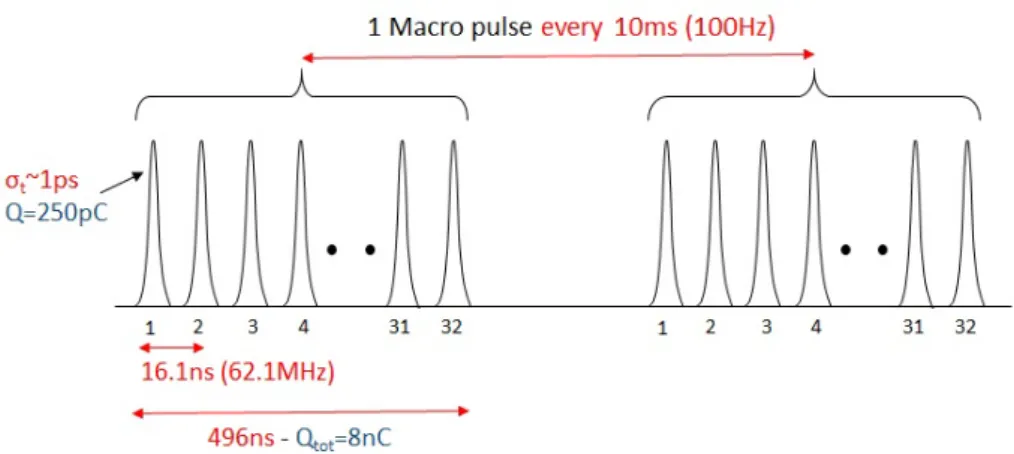
Macro repetition rate 100 Hz

# of pulses per macropulse ≤ 32

Pulse to pulse separation 16 ns

To reach these challenging specifications, in particular the high value of spectral density, an innovative interaction point module, used for the collision between the electron beam and the laser was designed. The laser pulses generated (see Table 1.2 for the main specifications) are recirculated 32 times at the interaction point within the Interaction Point Module, in order to collide with a multi-bunch electron beam pulses (constituted by 32 bunches, separated by 16.1 ns). A detailed analysis and description of this new optical device can be found in [10], while a general description of the linac will follow in section 1.2 and can be further deepened in [11].

Table 1.2: Summary of Laser Pulse specifications at the interaction points of ELI-NP GBS

Pulse Energy 0.2 – 0.4 J

Wavelength 515 nm

Energy 2.4 eV

Pulse Length (rms) 1.5 ps

Laser M2 _1.2

Pulse Repetition Rate 100 Hz

Waist 28.3 µm

Collision Angle 172°

Passes through the interaction point 32

ELI-NP GBS will be one of the most performing devices in producing radiation with short wavelength, high power, ultrashort time duration, large transverse coherence and tunability. Since the photon energy gain factor in the high energy inverse Compton scattering mainly depends on the energy of the colliding electron beam, the photon beam energies can be easily extended to cover a wide range from soft X ray to very high

(9)

8

energy gamma ray. Another advantage of Compton sources is that secondary photons emitted by inverse Compton scattering present an energy-angle correlation. Thus, by using a collimation system, it is possible to obtain a quasi-monochromatic photon beam, while the forward focusing ensures high spectral densities in small bandwidths.

(10)

9

(11)

10

1.1 _{Interaction points and Cavity BPMs}

At ELI-NP GBS, two interaction points module are foreseen: one for electron energies up to 280 MeV and the other for energies up to 740 MeV. In both modules (which share the same layout), the laser is recirculated up to 32 times in order to collide with the electron beam, constituted by trains of 32 bunches. The laser is injected in the module and will be reflected by means of two Parabolic Mirrors and 31 Mirror Pair Systems, intercepting the interaction point with an angle of 172° in respect to the electron beam (see Figure 1.2) [10].

Figure 1.2: Schematic top view of the interaction point module. The green trace represents the laser recirculated 32 times through two parabolic mirrors (M1, M2) and the Mirror Pair System (MPS) [10].

The gamma rays are produced by means of inverse Compton back-scattering. The scattered photon energy Eg is given by [13]:

𝐸𝐸𝑔𝑔 = (1 − 𝛽𝛽 cos 𝜃𝜃𝑖𝑖)𝐸𝐸𝑝𝑝ℎ

�1 − 𝛽𝛽 cos 𝜃𝜃𝑓𝑓� + �1 − cos 𝜃𝜃𝑝𝑝� 𝐸𝐸𝑝𝑝ℎ⁄𝐸𝐸𝑒𝑒𝑒𝑒

(1.1)

where β is the speed of the incident electrons relative to the speed of light; θi is the

polar angle between the incident photons and electrons directions; θf is the scattering

angle of the photons; θp is the polar angle between the incident and scattered photons

directions and is equal to θi - θf; Eph is the incident photons energy; Eel is the electrons

(12)

11

Figure 1.3: Representation of Compton scattering from the collision of an electron beam and incident photons.

To adapt the formula for ELI-NP GBS we can consider the nominal values for the following quantities: Eel = 740 MeV (maximum value), Eph = 2.4 eV, θi = 172°. By fixing

this quantities, it is possible to show the relation between the scattered photon energy Eg and the scattering angle θf, plotted in Figure 1.4 [14].

Figure 1.4: Relation between the scattered photon energy (Eg) and the scattering angle

(θf), for a simulated Compton scattering with the nominal parameters of ELI-NP GBS.

It is possible to see that, with a good approximation, the maximum energy (about 19.5 MeV) is obtained for θf = 0 and that the higher is the scattering angle, the lower is

the photon energy. The energy is independent from the azimuth angle. Thus, by using an observation plane downstream from the collision point and perpendicular to the electron beam direction, photons of equal energies would be disposed in concentric circles [13]. From a practical point of view this energy distribution is exploited in ELI-NP

(13)

12

GBS by using a gamma-ray collimator in order to achieve a scattered photon beam with a small energy spread. The intensity of the scattered photons is also dependent on the scattering angle. The maximum intensity is achieved at θf = 0 and decrease for higher

values of θf [13].

Given the dependency of Energy and Intensity from the scattering angle and the tight specifications on the gamma beam (see Table 1.1), an alignment system for the Interaction Point module and the collimators is foreseen. Precise position measurements of the electron beam at the interaction point are also mandatory. The problem is not only to the transversal position of the electron bunches, which should be optimized to fully intercept the recirculated laser, but also for the angle of the electron beam, that is important for the energy and spatial distribution of the gamma rays produced. To fulfil this requirements, Cavity BPMs will be installed immediately before and after the two Interaction points modules, as depicted in Figure 1.5. This would give the opportunity to measure the position and the angle of the beam at the Interaction points for each of the 32 bunches of the electron macro pulses. The resolution requirement for the transversal beam position, as measured by the Cavity BPM, was estimated to 1 µm, over a measurable range of ±1 mm.

Figure 1.5: 3D view of the complete interaction point module. Cavity BPMs are installed immediately before and after the module [10].

(14)

13

1.2 _{ELI-NP-GBS LINAC overview}

The Gamma Beam System (GBS) [2] is based on a warm RF linear accelerator operated at the C-band mode, with S-band photo-injector. The general layout of the machine is shown in Figure 1.1. The linac will deliver electron beams in the energy range of 80 – 740 MeV. It will operate at 100Hz repetition rate with trains of 32 electron bunches, separated by 16.1 ns and a 250 pC nominal charge (see Figure 1.6). The requirements of the electron beam at Interaction Points are reported in Table 1.3.

Figure 1.6: ELI-NP GBS electron beam representation in multi-bunch operation mode.

There are two stages, the first stage will produce electrons with energy up to 280 MeV (low energy line), and the second stage the electrons will be accelerated up to 740 MeV (high energy line). At the end of both energy lines, the two Interaction Point Modules are foreseen. The electron beam at the GBS will be generated in the laser-driven photocathode mounted in 1.6 cell standing-wave cavity what all together constitutes the RF gun. It will operate with high electric field gradients 120 MV/m. By illumination of the cathode with laser pulses, the electron bunches, each with the length of 10 ps, will be emitted. The high gradient of radio-frequency field will provide rapid acceleration to relativistic energies. In the first two travelling wave accelerating structures the beam will gain the energy approximately 80 MeV. These are the constant gradient (22 MV/m) structures and will operate at 2.856 GHz (S-band), with the cell phase advance of 2π/3. They will also act as a bunch compressor, decreasing the bunch length from 10 ps to 1 ps, by employment of the velocity bunching.

The linac booster will be composed of 12 travelling wave structures working at 5.712 GHz (C-band) in TM01 mode with the cell phase advance of 2π/3, and

(15)

quasi-14

constant accelerating field gradient 33 MV/m. For a deepening on the Linac, refer to [11].

Table 1.3: Summary of Electron Beam Parameters at Interaction Points of ELI-NP GBS

Energy 80 – 740 MeV

Bunch Charge 25 – 250 pC

Bunch Length 100 – 400 µm

εn_x,y 0.2 – 0.6 mm·mrad

Bunch Energy spread 0.04 – 0.1 %

Focal Spot Size > 15 µm

# of bunches in the train ≤ 32

Bunch separation 16 ns

Energy Variation along the train 0.1 % Energy jitter shot-to-shot 0.1 % Emittance dilution due to beam

break-up < 10 %

Time Arrival Jitter < 0.5 ps

(16)

15

2 Diagnostics for ELI-NP GBS

2.1 Overview

Various diagnostics devices have been foreseen to be installed in the LINAC, in order to measure the properties of both the macro-pulses and the single bunches. The devices used for the intercepting type of measurements are Optical Transition Radiation (OTR) and YAG screens. A total of 23 stations will be installed along the LINAC: 12 on the Low Energy LINAC, 11 on the High Energy LINAC. They will be used to measure the Beam Position (Centroid) and the Spot Size of the beam. They will also be used to measure the beam energy and its spread, the bunch length and the Twiss parameters, in conjunction with a dipole, an RF deflector and quadrupoles respectively [15]. The devices used for non-intercepting measurements are Beam Charge Monitors (BCM) and Beam Position Monitors (BPM) (see Figure 2.1). The former ones are based on the Integrating Current Transformers (ICT) [2], which will be installed in 4 different positions (3 in the low energy LINAC, 1 in the high Energy LINAC). Concerning the Beam Position Monitors, two different types will be installed: Stripline Beam Position monitors are the most common. 29 of them will be installed, specifically 13 in the Low Energy LINAC, 16 in the High Energy LINAC. Near the interaction points (both at low energy and high energy), a total of 4 Cavity Beam Position Monitors will be installed.

A quick overview of the non-interceptive diagnostics used in ELI-NP GBS is described in the next sections.

(17)

16

Figure 2.1: Simplified layout of ELI-NP GBS. Both dump lines after the interaction points and some accelerator components are not depicted (e.g. corrector magnets and beam screens).

(18)

17

2.2 Beam Charge Monitors

Beam charge monitors (BCM) will be installed in four positions: the first one will be located right before the first S-band accelerating structure; the second one will be located at the end of all the accelerating structures of the Low Energy LINAC, before the so-called “dogleg”; the third and the fourth will be installed before the low energy and the high energy interaction points. These four locations will allow studying the losses of charge of the beam at the key-points of the LINAC.

Figure 2.2: Integrating Current Transformer from Bergoz Instrumentation for ELI-NP GBS.

BCMs will have the capability to measure the charge of every single bunch, within the macro pulse. The devices which will be installed along the linac are the Integrating Current Transformers (ICT) from Bergoz Instrumentation (see Figure 2.2), whose specifications are reported in Table 2.1. The ICT generates a pulse signal with a nominal duration of 5 ns when a beam bunch pass through it. By integrating the pulse and applying a scale factor (the inverse of the ICT Sensitivity), it is possible to calculate the bunch charge, as shown in Eq. (2.1).

𝑄𝑄𝑏𝑏𝑏𝑏𝑏𝑏𝑏𝑏ℎ =1_{𝑆𝑆 ∗ � 𝑉𝑉}𝑜𝑜𝑏𝑏𝑜𝑜(𝑡𝑡)𝑑𝑑𝑡𝑡 16𝑏𝑏𝑛𝑛

0

(2.1)

The ICT operates as a band-pass filter on the signal generated by the passage of a beam bunch through the toroid. The latter could be considered as the input signal of the system. As such, a bunch of ~1 ps will induce an output signal with a duration of 5 ns, by maintaining a proportionality between the charge of the output signal and the charge

(19)

18

of the bunch. The duration of the output signal is short enough to measure the charge bunch by bunch.

Table 2.1: Main parameters of the ICTs for GBS. In parenthesis the measured values in laboratory.

Parameter Value

Sensitivity (S) in a 50Ω load _{(4.96 Vs/C)}5 Vs/C Beam charge to output charge ratio in

50Ω load ~10:1

Output pulse duration (6σ) _{(5.6 ns)}5 ns Output signal droop _{(3.57 %/ µs)}3.59 %/µs

flow / fhigh _{(4.5kHz/180MHz)}5.3kHz/191MHz

The output signals are digitized with 10bit 4GS/s ADC (Agilent M9210A) and processed by a cPCI crate embedded system with a dedicated control software written in EPICS. The latter will calculate the charge for each bunch window, by applying a calibration factor and offset compensation chosen by the user. For a detailed overview of the system refer to [15].

2.3 _{Stripline Beam Position Monitors}

A total of 29 Stripline BPMs will be installed in ELI-NP GBS. They are the main devices used to measure the average position of the macro pulse along the LINAC. The design is the same for all of them (Figure 2.3), except for the one installed on the dump line after the low energy interaction point, which was designed in order to have a larger beam acceptance range (Ø100 mm) [15].

Stripline BPMs are composed of four stainless steel electrodes of length L = 140mm and width w = 7.7 mm, mounted with a π/2 rotational symmetry at a distance d = 2mm from the vacuum chamber, to form a transmission line of characteristic impedance Zo=50 Ω with the beam pipe. Their acceptance is Ø34mm.

The amplitude of the frequency response presents a sinusoidal shape with maxima at odd multiples of c/4L (~535MHz), selected to be as close as possible to the operating

(20)

19

frequency of the detection electronics and to present non-zero response at the LINAC frequency of 2856 MHz.

Figure 2.3: Stripline BPM schematics for ELI-NP GBS.

The read-out electronics is represented by Instrumentation Technologies “LIBERA Single pass E” modules. The latter provides analogue front-end electronics to handle the pulse-like signals generated by the passage of the beam on the striplines. The signals are then digitized and processed by an FPGA, in order to calculate the average position of each train of bunches. Horizontal and vertical positions are calculated in first approximation with a difference over sum algorithm applied to the measured amplitude of the signals coming from the corresponding pair of striplines (horizontal and vertical). For ELI-NP GBS, in order to use the full BPM acceptance area without accuracy losses due to non-linearities, we plan to use correction algorithms, developed on the basis of simulations and measurements of BPMs response. In particular, suitable high-order surface polynomials will be used. The calibration factors, used in the polynomial equations, will be extrapolated from the measurements and calibration performed at ALBA laboratories [16] for each BPM and will be implemented directly in the LIBERA Single Pass E modules.

There is also the plan to calculate the charge of each train of bunches by using the output signals of the BPM, in order to increase the number of the charge measurements all along the LINAC [17].

(21)

20

2.4 Cavity Beam Position Monitors

The importance of having high resolution measurements for the beam position at the Interaction points was discussed in section 1.1. Cavity BPMs were selected as the devices which could guarantee the best performances, also in presence of low charge beams, in terms of position resolution for bunch by bunch measurements. Moreover, they give the possibility to measure the charge of each bunch. The cavity pick-up is the PSI BPM16 model, consisting of two resonators with low quality factor (Q = 40) and a resonance frequency of 3.3 GHz [18],[19].

Figure 2.4: Picture of the Cavity BPM model PSI BPM16 used for ELI-NP GBS

The low Q allows to measure the charge and the position of the beam bunch by bunch. In fact, the output signals associated to the passage of a single bunch will decay faster than the time interval between bunches (16 ns). An in-depth discussion of the working principles and features is presented in Chapter 3.

The readout electronics has been specifically designed for the cavity BPM of ELI-NP GBS in collaboration with Instrumentation Technologies. A detailed description of the read-out electronics, as well as the characterizations performed in laboratory and in presence of beam are discussed in Chapter 4, 5, 6.

(22)

21

3 Cavity Beam Position Monitors

The basic idea of the Cavity Beam Position Monitor (cBPM) is quite old, which backs to 1960’s. When SLAC was built, this type of BPMs were installed in the drift session along the accelerator and in the beam switchyard [20]. From that time, various configuration of BPM cavities and read-out electronics have been developed in many laboratories and widely used to monitor the beam trajectory mostly in linacs. The type of cBPM that will be discussed in this dissertation is one of the most diffused and is based on the presence of two pillbox cavities.

3.1 _{Theory and Working principle}

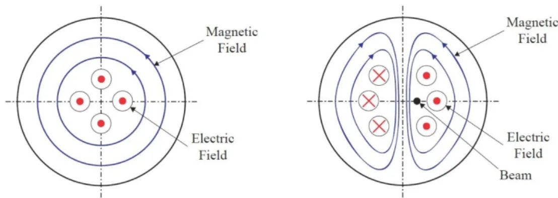
Cavity BPM is based on the resonant modes excited in the pillbox cavities when a bunch transit through them. For a cavity with L < 2.03R, where L is its length and R is its radius, the monopole mode TM010 is the fundamental oscillation of the cavity [21]. For beams

near the center of the cavity, the monopole mode is symmetric and is proportional to the charge of the excitation bunch (see Figure 3.1, left picture). This constitutes the first piece of information used for the beam position calculation, as will be described later. The beam bunch will excite also higher order modes of the cavity, in particular the dipole mode TM110. Its amplitude has a linear dependence on the charge of the bunch as well

as on the transverse offset of the beam relative to the electromagnetic (e.m.) center of the cavity. Its phase depends on the direction of the beam offset.

Figure 3.1: Representation of a pillbox cavity section. The electromagnetic fields of the

TM010 (left) and TM110 (right) modes are shown, as excited by the passage of a beam

(23)

22

Beam position calculation is based on the measurements of the amplitudes of these two modes. Two cavities, placed one after the other in respect to the beam direction, are used: one, named “reference” cavity (or resonator) to measure the amplitude of the monopole mode; the other, named “position” cavity to measure the amplitude of the dipole mode. The monopole mode measurement is used as a reference for two reasons: 1. the amplitudes of the two modes are compared (i.e. the ratio is calculated) in order to obtain a quantity which is dependent only on the beam position, regardless of the bunch charge.

2. The phase of the two modes are compared in order to obtain the direction of the beam offset. This is possible because the monopole mode has always the same phase, while the dipole mode phase depends on the direction of the beam offset.

The explicit expressions for the fields of the TM010 (eq.(3.1)) and TM110 (eq.(3.2)) are

reported in [20] and [21], for the simple case of a pillbox cavity with radius R and length L. These expressions can be considered an approximation of the real case, because they do not take into accounts the presence of the beam pipe and of the waveguides (see later on this paragraph) or other factors, such as the crosstalk between the fields excited in the two cavities. For a short introduction on pillbox cavities for particle accelerators, refer to [22]. 𝐸𝐸𝑧𝑧 = 𝐴𝐴 · 𝐽𝐽0(𝑗𝑗01𝑟𝑟) · 𝑒𝑒𝑖𝑖𝜔𝜔010𝑜𝑜 𝐻𝐻𝑟𝑟 = 0 𝐻𝐻𝜙𝜙 = −𝑖𝑖𝐴𝐴 · 𝑗𝑗_𝜔𝜔 01 010𝜇𝜇 · 𝐽𝐽1 ′_(𝑗𝑗 01𝑟𝑟) · 𝑒𝑒𝑖𝑖𝜔𝜔010𝑜𝑜 (3.1) 𝐸𝐸𝑧𝑧 = 𝐴𝐴 · 𝐽𝐽1(𝑗𝑗11𝑟𝑟) · cos(𝜙𝜙) 𝑒𝑒𝑖𝑖𝜔𝜔110𝑜𝑜 𝐻𝐻𝑟𝑟 = −𝑖𝑖_{𝜔𝜔𝜇𝜇 ·}𝐴𝐴 𝐽𝐽1(𝑗𝑗_𝑟𝑟11𝑟𝑟)· sin(𝜙𝜙) 𝑒𝑒𝑖𝑖𝜔𝜔110𝑜𝑜 𝐻𝐻𝜙𝜙 = −𝑖𝑖𝐴𝐴 · 𝑗𝑗_𝜔𝜔 11 110𝜇𝜇 · 𝐽𝐽1 ′_(𝑗𝑗 11𝑟𝑟) · cos(𝜙𝜙) 𝑒𝑒𝑖𝑖𝜔𝜔110𝑜𝑜 (3.2)

J0 and J1 are the Bessel functions of the first kind of order 0 and 1; j01 and j11 are their

roots; ω010 and ω110 are the resonant angular frequencies, calculated with eq.(3.3),

(24)

23 𝜔𝜔𝑚𝑚𝑏𝑏𝑝𝑝 = 𝑐𝑐��𝑗𝑗𝑚𝑚𝑏𝑏_{𝑅𝑅 �}

2

+ �𝑝𝑝𝑝𝑝_{𝐿𝐿 �}2 (3.3)

A0 and A1 are equal to E0/J0max and E1/J1max. J0max and J1max are the maximum value of

the Bessel functions and E0, E1 are the maximum value of the electric fields at a radius

(rl) corresponding to the maximum of the Bessel function (refer to Figure 3.2).

Figure 3.2: Representation of the excitation of the monopole and dipole mode at the passage of a beam bunch. The dipole mode is excited only if the beam has an offset in respect to the electromagnetic center of the cBPM.

To calculate how the modes of the cavity are excited by the beam bunch, we need to calculate the energy released by the latter. This depends entirely on the geometry of the cavity and the properties of the bunch (i.e. in first approximation, direction, offset and charge). The key parameter for the cavity is the normalized shunt impedance, defined as:

𝑅𝑅 𝑄𝑄 =

𝑉𝑉2

𝜔𝜔𝜔𝜔 (3.4)

where W is the energy transferred and stored in the cavity and the potential V is defined as:

𝑉𝑉 = �� 𝐸𝐸𝑧𝑧𝑑𝑑𝑑𝑑 𝐿𝐿_�₂ −𝐿𝐿_�₂ �

(3.5)

By calculating the energy transfer from the beam bunch to an initially empty cavity, it is possible to calculate the voltage Vout (eq.(3.6)) in an output line with impedance Z

(25)

24

(assuming the presence of properly designed couplers). Refer to [20] and [21] for a full explanation. 𝑉𝑉𝑜𝑜𝑏𝑏𝑜𝑜 =𝑞𝑞 · 𝜔𝜔₂110�_𝑄𝑄𝑍𝑍 𝑒𝑒𝑒𝑒𝑜𝑜� 𝑅𝑅 𝑄𝑄�_𝑚𝑚· 𝑇𝑇(𝜃𝜃) · 𝐽𝐽1(𝑗𝑗11𝑟𝑟) 𝐽𝐽_{1𝑚𝑚𝑚𝑚𝑒𝑒} sin(𝜔𝜔110𝑡𝑡) 𝑒𝑒−𝑜𝑜/𝜏𝜏 (3.6) Qext is the external-Q of the external coupling; (R/Q)m is the shunt impedance defined

for the potential calculated with the maximum electric field E1; T(ϑ) is the transit time

factor (usually negligible); τ is the decay constant equal to:

τ =2𝑄𝑄_𝜔𝜔𝐿𝐿 (3.7)

where QL is the loaded Q.

For beam around the electromagnetic center, the Bessel function J1(j11r) is proportional

to the beam offset. Thus, Vout is a sine signal, decaying in time, whose amplitude can be

used to measure the beam position (see Figure 3.3)

Figure 3.3: Simulation of the cBPM output signal associated to the excitation of the dipole mode. The signal is a sinewave, decaying in time, whose amplitude is proportional to the beam charge and offset of the beam bunch. The parameters which define the signal (frequency and decay constant) depends on the geometry of the cavity and on its

QL. The simulation is based on the parameter of the cBPM used for ELI-NP GBS (see

section 3.2)

The dipole mode is also dependent on the beam angle. In commonly used beam optics, the signal level dependent on the beam angle is usually much smaller than the beam

(26)

25

position signal. Nevertheless, it should be taken into consideration, as it could bring to problems on the measurement accuracy of the beam position. An analysis of the angle dependency can be found in [20] and [21], while a detailed analysis of the response of Cavity BPM to more complex beam profiles is discussed in [23].

Concerning the dipole mode, it is possible, by taking advantage of the horizontal and vertical polarization of the fields and with an adequate design of the cavity, to measure the horizontal and vertical displacement separately.

One possible design is illustrated in Figure 3.4. Four rectangular waveguides are matched to the position cavity by coupling ports. Due to their geometric configuration the X-ports will couple only with the X dipole mode, rejecting the Y dipole mode and the monopole mode; same applies for the Y-port (Figure 3.5).

Figure 3.4: Cavity BPM schematic view [18].

Figure 3.5: Representation of a pillbox cavity section with magnetic (blue) field lines. Due to their geometry, the X-ports will couple only with the X dipole mode, rejecting the Y dipole mode and the monopole mode. Same applies for the Y-port.

(27)

26

Antennas, connected to a coaxial output, are placed inside the waveguides and will couple with the field of the extracted mode. The reason to use four waveguides, two for X and two for Y, is to keep the symmetry of the cavity BPM. Moreover, it is possible to sum the signals in pairs, once extracted, doubling the amplitude of the final signal for X and for Y and to further reduce the contribution of the monopole mode on them.

The reference cavity is simpler in design. Antennas are directly inserted in the cavity, without the implementation of waveguides. This is due to the fields distribution within the cavity and the fact that the monopole mode is the fundamental one (i.e. the contribution of higher order modes to the output signal is marginal).

The output signal is similar in shape as the one descripted for the dipole mode (see Figure 3.3), with the exception that its amplitude is proportional only to the bunch charge.

In general, the radius of the two resonators is chosen in such a way that the resonance frequencies of the monopole mode for the reference cavity and the dipole mode for the position cavity are the same. Thus, the two signals have the same frequency facilitating the design of the readout electronics and simplifying the measurement of the phase difference between the two signals. For general readings on cBPM and their related performances, refer to [24], [25],[26] and [27]. For an example of the design process of a cBPM and its related issues refer to [28] and [29].

3.2 _{Cavity Beam Position Monitors for ELI-NP GBS}

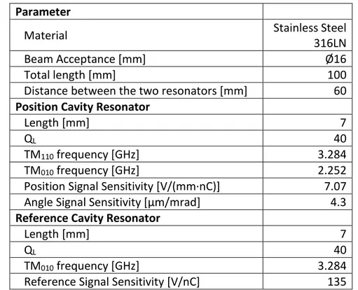
Cavity Beam Position Monitor (cBPM) that will be used for ELI-NP GBS is the PSI model “BPM16”. This model was designed for the SwissFEL linac, but its features fit well for the ELI-NP GBS implementation. Thus, four additional cBPMs were produced in collaboration with PSI and delivered at INFN-LNF. A detailed description and analysis of their design can be found in [18] and [19].

The main nominal parameters of the cBPM are reported in Table 3.1, while a picture and a 3D model are reported in Figure 2.4 and Figure 3.6. The cBPM has five N-type connectors, two for signals associated to position X (carrying the same signals), two for position Y and one for the reference signal.

(28)

27

Figure 3.6: Layout and 3D representation of the cBPM PSI model “BPM16”. Courtesy of B.Keil. There are two ports for X and Y, which can be used independently.

Table 3.1: Main parameters of the cBPM, PSI model “BPM16”, used for ELI-NP GBS.

Parameter

Material Stainless Steel _316LN Beam Acceptance [mm] Ø16

Total length [mm] 100

Distance between the two resonators [mm] 60

Position Cavity Resonator

Length [mm] 7

QL 40

TM110 frequency [GHz] 3.284

Position Signal Sensitivity [V/(mm·nC)] 7.07 Angle Signal Sensitivity [µm/mrad] 4.3

Reference Cavity Resonator

Length [mm] 7

QL 40

Reference Signal Sensitivity [V/nC] 135

The main reason to use this cBPM model is related to the low loaded quality factor. As described in Eq. (3.7), by taking into account that QL = 40 and ω = 2π·3.284 GHz, the

resulting decay constant of the output signals, for both resonators, is τ = 3.87 ns, which is lower than the time interval between bunches in ELI-NP GBS (16.1 ns). Nevertheless, a small portion of each signal, associated to the passage of a single bunch (the “tail”), will interfere with the signal of the subsequent bunch. This issue and its solution will be later described in section 4.2.2. The PSI model “BPM16” has a high enough position

(29)

28

signal sensitivity (see Table 3.1) to be applicable for ELI-NP GBS. Results obtained at SwissFEL [30], show that a resolution of 1 µm for beam bunch charges as low as 10 pC are obtainable.

Preliminary radio-frequency measurements performed at PSI for the four cBPM to be used in ELI-NP are reported in Table 3.2.

Table 3.2: Radio-frequency measurements of the cBPM, PSI model “BPM16”, used for ELI-NP GBS, performed at PSI. Results were obtained by measuring the scattering parameters of the five ports.

Parameter fres [GHz] QL cBPM no. B-004 X-plane 3.2897 43.1 Y-plane 3.2901 42.1 Reference 3.2793 37.5 cBPM no. B-012 X-plane 3.2881 42.3 Y-plane 3.2881 43.3 Reference 3.2774 38.3 cBPM no. B-013 X-plane 3.2894 43.3 Y-plane 3.2886 42.4 Reference 3.2809 38.4 cBPM no. B-014 X-plane 3.2889 41.9 Y-plane 3.2891 42.8 Reference 3.2793 37.8

Table 3.3: Average and maximum variation of the resonance frequency and QL for the reference and position resonators.

Position

Resonator Resonator Reference

Mean fres [GHz] 3.2890 3.2792

Variation range of fres [GHz] 0.0020 0.0035

Mean QL 42.65 38

Variation range of QL 1.4 0.9

In Table 3.3, the average values and the maximum variation for the resonance frequency and loaded Q are reported for both resonators, taking into accounts the measurements performed on the four Cavity BPMs. The small differences for these parameters could be considered negligible for the position measurements.

(30)

29

4 Readout Electronics for Cavity BPM

Readout Electronics design is of critical importance in a Cavity Beam Position Monitor measuring system. This is due to the fact that if not carefully designed, the accuracy, the resolution and the repeatability of the measures can be heavily affected, reducing the overall performance of the measuring system. The readout electronics main task is to collect signals from the Cavity BPM, elaborate them and present an estimation of the beam position.

The majority of readout electronics used for Cavity BPMs is nowadays based on the down-conversion of the Cavity BPM signals and the digital transformation of them, by means of Analog to Digital Converters (ADC). The digital signals will then be elaborated in order to present the estimation of the beam position. Different signal processing schemes can be adopted in order to do so. One of the most used is based on the I-Q demodulation, which will be described later.

The readout electronics which will be implemented in ELI-NP GBS for the Cavity BPMs is represented by the “LIBERA Cavity BPM” modules, recently developed (2017) by Instrumentation Technologies (Figure 4.1) [31],[32],[33]. The initial concept and the development were elaborated and executed by taking into accounts the ELI-NP GBS requirements. The development and the final stage of testing and validation where performed in strict collaboration with INFN-LNF and represent part of the work discussed in this thesis.

The module has three independent input channels (SMA connectors), named “X”, “Y”, “I”, which are used for the output signal coming from a single Cavity BPM. “X” and “Y” are used for the signals of the “position” resonator, “I” is used for the reference resonator. The channels and the related electronics are the same for each channel. The only difference is related in how the digital data related to the signals are used to compute the beam position. The signals are filtered, down-mixed and attenuated/amplified by means of front-end electronics, independently for each channel. They are then digitized and the beam position is calculated with algorithms performed by an FPGA. An external trigger is used to synchronize the acquisition with the beam bunches. The module needs also an external reference signal, i.e. a sinewave with the same frequency of the bunches (62.087 MHz), that is in common for the three channel and is used to down-mix the input signals and to lock the ADC sampling frequency. A full explanation of all the sub-systems of the module will follow in the next sections, while the main parameters of it are shown in Table 4.1.

(31)

30

Table 4.1: Main parameters of the “LIBERA Cavity BPM”.

Parameter General

Number of RF inputs 3

Input connector type SMA Maximum Input Range 16 dBm Signal Frequency for ELI 3.3 GHz

FPGA /CPU (model) Zynq-7035 / Dual Core ARM _{Cortex –A9} ADC (model) Analog Device AD9680-500

Channels no. 4

Number of bits 14

Bandwidth 2 GHz

Sampling Rate 500 MS/s

Maximum Input Range 2.06 Vp-p

Trigger signal Single Ended lvTTL

Trigger connector type LEMO Max. Trigger frequency 100 Hz Trigger frequency for ELI 100 Hz

Reference Signal Continuous sine-wave Ref. Signal connector Type SMA Signal Level Range 0-10 dBm Signal frequency for ELI 62.087 MHz

Figure 4.1: “LIBERA Cavity BPM”, developed by “Instrumentation Technologies” as the readout electronics for Cavity BPM signals. Front and back panels view.

(32)

31

4.1 Front end electronics and digitizer

The working principle of the front end electronics can be explained by looking at Figure 4.2.

Figure 4.2: Block diagram of “LIBERA Cavity BPM” [32].

Each module is capable to acquire the signals produced by the “position” resonator (“X”, “Y”) and by the “reference” resonator (“I”) of one Cavity BPM.

4.1.1 Variable attenuators

At the front-end stage, the signals are filtered from unwanted frequency component and their amplitudes are adjusted by means of variable attenuators (0 dB / 32 dB), depending on the beam conditions (e.g. charge, position). After the variable attenuators, a series of fixed-gain amplifiers [33] and internal attenuators are used to further adjusting the signals level (not depicted in Figure 4.2).

The choice of the attenuation levels plays an important role in the determination of the resolution of the measurements. The main objective is to adjust them in order to exploit all the dynamic range of the read-out electronics and at the same time avoiding the saturation of the channels. For example, by knowing the maximum possible charge of the bunches during a specific accelerator operation, it is possible to adjust the attenuators of channel “I”, in such a way that with the maximum bunch charge, the

(33)

32

signal on the “I” channel will take 90% of the input range. This will improve the Signal to Noise ratio (SNR) and will help to achieve the best resolution possible on the measurement. For channel “X” and “Y”, the choice relies not only on the maximum charge of the bunches, but also on the maximum observable range of the bunch position. Once the maximum bunch charge is fixed, it is possible to choice the maximum observable range, by selecting the attenuations of “X and “Y” channels (the higher the attenuation chosen, the higher the observable range). By selecting low attenuation values, the maximum observable range will decrease, but (since the signal will have higher amplitudes) the SNR will increase and so will do the resolution of the system. As such, adjusting the attenuators gives the possibility to the user to adjust the level of the resolution wanted at the cost of the maximum observable range. This holds true if two conditions are verified.

•_{Noise introduced by the read-out electronics is dominant, if compared to the} thermal noise inherent to the Cavity BPM (see section 5.2). In the opposite case, SNR is fixed, irrespective to the attenuation used.

•_{The Cavity BPM signals are strong enough (depending on the charge and} position of the beam) to cover at least 100% of the input range of the readout electronics channels (without the use of attenuations). If this not holds, the attenuation level should be simply put to zero in order to exploit the input range at best.

Concerning the second point, each channel of the “LIBERA CavityBPM” has an input range of -15 dBm (Vmax= ±56 mV) without any attenuation. The sensitivity of the

resonators of the ELI-NP GBS Cavity BPM are S = 7.07 V/nC/mm and S = 135 V/nC (see Table 3.1).

As such, for example, with bunches of 100 pC and transversal beam offsets in the order of hundreds of µm (which is a realistic case for the foreseen operation at ELI-NP GBS), the signals would be strong enough to cover more than the maximum input range of all the channels of the “LIBERA Cavity BPM”.

4.1.2 Down conversion and digitization

Down-conversion is applied to the cBPM signals by using the reference signal provided to the system. The main reason to down-mix the signal is to relax the requirements on the ADC.

(34)

33

The reference signal (“Ref”) at the bunch repetition frequency (62.087 MHz) is provided by the timing system to two Phase Locked Loops (PLLs) (refer to [35],[36]), which generate the ADC sampling frequency (fADC = 496.7 MHz) and the

down-conversion mixer components (fLO = 3.663 GHz). The cavity input signal (fres = 3.284 GHz

with a bandwidth of 82.1 MHz) is adjusted by a series of attenuators and amplifiers (not depicted in Figure 4.2) and down-converted to an intermediate frequency (fIF = 379 MHz

with a bandwidth of 82.1 MHz).

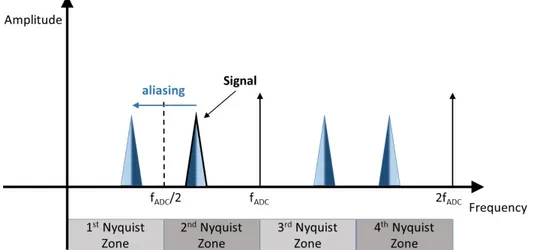
It should be noted that the sampling frequency is not high enough to satisfy the Nyquist criterion. In fact, the signal is under-sampled, falling in the second Nyquist zone, which is delimited by fADC/2= 248.5 MHz and fADC=496.7 MHz, as shown in Figure 4.3 [37], [38].

A band-pass filter centered at 375 MHz with a bandwidth of 116 MHz is used to ensure that all the harmonic contents of the signal falls entirely into the second Nyquist zone. The effect of under-sampling in the second Nyquist zone is that the digitized signal is an aliased representation of the analogue signal. This means that the digitized signal will have a central frequency (aliased representation of the central frequency of the analogue signal) of:

𝑓𝑓𝑚𝑚𝑒𝑒𝑖𝑖𝑚𝑚𝑛𝑛 = 𝑓𝑓𝐴𝐴𝐴𝐴𝐴𝐴− 𝑓𝑓𝐼𝐼𝐼𝐼 = 117.7 𝑀𝑀𝐻𝐻𝑑𝑑 (4.1)

It should also be noted that by the effects of under-sampling, the frequency content of the aliased representation is inverted compared to the analogue signal frequency content (see Figure 4.3). Nevertheless, by the Nyquist-Shannon sampling theorem, it is possible to fully reconstruct the original signal perfectly from the sampled version.

Figure 4.3: Representation of the Nyquist zones and the effects of the under-sampling

technique (aliasing). fADC/2 is half of the sampling frequency and coincides with the

(35)

34

The “T2” input (see Figure 4.2) is used for the machine trigger (100 Hz) and it is used to start the acquisition procedure.

The ADC data is continuously transferred through serial interfaces to a Xilinx ZYNQ 7035 System on Chip, which provides all the necessary computing resources, including a FPGA, a CPU and the internal shared memory. Every time a new injection happens, the trigger signal enables the storage of up to 4096 ADC samples in the memory of the device, ready to be further processed.

4.2 Digital processing

Figure 4.4: Block diagram of “LIBERA Cavity BPM” data-paths

4.2.1 Calculation of the beam position

Once the signals are digitized, their amplitudes is computed. For each channel (“X”, ”Y”, ”I”) the samples are organized in “bunch windows” which are used to calculate the amplitude (VXb, VYb, VIb) of the signals associated to the bth bunch. The number of

samples composing a single “bunch window” is adjustable, but during the multi-bunch operation mode in ELI-NP GBS should be fixed at eight, due to the time structure of the beam.

(36)

35

Figure 4.5: Position Calculation block scheme for “X” and “I” channels.

The amplitudes of the signals are calculated as:

𝑉𝑉_{𝑋𝑋𝑏𝑏}_{= �} � 𝑥𝑥𝑏𝑏2 𝑏𝑏𝑜𝑜ℎ 𝑏𝑏𝑏𝑏𝑏𝑏𝑏𝑏ℎ 𝑤𝑤𝑖𝑖𝑏𝑏𝑤𝑤𝑜𝑜𝑤𝑤 𝑉𝑉_{𝑌𝑌𝑏𝑏} _{= �} � 𝑦𝑦𝑏𝑏2 𝑏𝑏𝑜𝑜ℎ 𝑏𝑏𝑏𝑏𝑏𝑏𝑏𝑏ℎ 𝑤𝑤𝑖𝑖𝑏𝑏𝑤𝑤𝑜𝑜𝑤𝑤 𝑉𝑉_{𝐼𝐼𝑏𝑏} _{= �} � 𝑖𝑖𝑏𝑏2 𝑏𝑏𝑜𝑜ℎ 𝑏𝑏𝑏𝑏𝑏𝑏𝑏𝑏ℎ 𝑤𝑤𝑖𝑖𝑏𝑏𝑤𝑤𝑜𝑜𝑤𝑤 (4.2)

In Eq. (4.2), xn, yn, in are the nth samples of the X, Y, I channels respectively. “bth bunch

window” is the sample window centered on the signals produced by the passage of the bth_{bunch. V}_Xb_{, V}_Yb,_V_Ib_{are proportional to the amplitude of the signal associated to the}

passage of the bth_{bunch. The absolute transverse position of each bunch is then}

obtained as (4.3): 𝑋𝑋𝑏𝑏= 𝐾𝐾𝑒𝑒𝑉𝑉_𝑉𝑉𝑋𝑋𝑏𝑏

𝐼𝐼𝑏𝑏 𝑌𝑌𝑏𝑏 = 𝐾𝐾𝑦𝑦

𝑉𝑉_{𝑌𝑌𝑏𝑏}

𝑉𝑉_{𝐼𝐼𝑏𝑏} (4.3)

Xb andYb are the calculated transverse distances of the bth bunch in respect to the

electromagnetic center (e.m. center) of the “position” resonator in the horizontal and vertical axes respectively. Kx and Ky are user-defined calibration constants which take

(37)

36

into accounts the sensitivity of the resonators, the level of input attenuator used and the attenuation of the cables. A calibration procedure is used to find the correct value for Kx and Ky before the starting of operations.

In order to evaluate the sign of the bunch position on the X and Y axes of the transversal plane, the phase of the signal of the X and Y channels are compared to the phase of the I channel (see section 3.1)

Thus, the samples in each bunch window are also used to calculate the phase of each signal: φX, φY, φI in relation to an internal generated signal. This is done through IQ demodulation applied to the samples in each bunch window. The phase is then calculated with the CORDIC (Coordinate Rotation Digital Computer) algorithm. Once φX-φI and φY-φI are calculated, it is possible to evaluate the sign of each bunch position. User-defined calibration constants are also applied in this case to compensate differences in the channel lengths, which could affect the calculated phase for each signal.

4.2.2 Deconvolution filter (for multi-bunch operation)

In multi-bunch operations, as previously described, the digitized samples are divided in bunch windows, each containing 8 samples (for ELI-NP GBS operations), for a total time interval of 16.1 ns. However, In the case of ELI-NP GBS, the resonators of Cavity BPMs produce signals at the passage of a bunch which will last over 16.1 ns, overlapping with the passage of the subsequent bunch. The amplitude of the “tail” of the signal which potentially overlaps is mainly determined by the Quality factor of the Cavity BPM resonators (QL= 40) and was calculated to be roughly 1.5% (see eq.(3.6) and (3.7)) of the

maximum amplitude of the signal after 16.1 ns. This potential problem could be worsened by the effects of cables used to bring the signal from the Cavity BPM to the readout electronics.

To reduce this inter-bunch interference, the digitized signals can be processed by a digital 100-bin FIR filter, called “Deconvolution” filter. This is used to limit the superposition between signals of consecutive bunches, by compressing them to occupy exactly 8 samples. An example of how the filter is defined and works with a single bunch input signal is presented in Figure 4.7.

(38)

37

Figure 4.6: Simulated signal shape of ELI-NP GBS Cavity BPM (“X” channels) in multi-bunch operation mode (the third multi-bunch is missing on purpose). It can be noted the small overlaps between signals from consecutive bunches. Amplitudes were simulated by taking into account a “Position” Resonator Sensitivity of 7.07 V/nC/mm for a bunch of 1 nC and a distance of 1 mm on the horizontal axis in respect to the electromagnetic centre of the Cavity BPM.

In order to define the Deconvolution filter response, a calibration procedure is needed before the starting of operations. In order to do this, a goal function has to be defined (G(t)). The latter was chosen to be a rise cosine shape as depicted in Figure 4.7. After that, an input signal produced by the passage of a single bunch in the cavity BPM should be provided (see Figure 4.7, INstd(t)). This is considered as the “standard” signal that the

cavity BPM will provide. The frequency and impulse response of the deconvolution filter are then calculated as:

𝐷𝐷𝐷𝐷(𝑓𝑓) =_{𝐼𝐼𝐼𝐼}𝐺𝐺(𝑓𝑓)

𝑛𝑛𝑜𝑜𝑤𝑤(𝑓𝑓) 𝑖𝑖𝐼𝐼𝐼𝐼𝑖𝑖

�� 𝐷𝐷𝐷𝐷(𝑡𝑡) (4.4) Where G(f) and INstd(f) are the Discrete Fourier transforms of G(t) and INstd(t) and iFFT

indicates the inverse of the Fast Fourier Transformation.

Thus, the deconvolution filter frequency response is calculated as the function that transforms the “standard” signal for the passage of a single bunch to a signal with a rise cosine shape, limited to 8 samples. The filter bins amplitudes are defined in order to guarantee that, once the filter is applied, the overall amplitude of the digitized signal Vx

(39)

38

Figure 4.7: Signals (simulated) involved in the calculation of the impulse response of the

deconvolution filter. The “standard” signal, Instd(t), is the signal produced by the passage

of a single bunch in the Cavity BPM. The Goal Function, G(t), is a user-defined rise cosine function. The Deconvolution Filter Impulse Response, DF(t), is calculated as the function

which transform Instd(t) into G(t).

Since the calculation of the deconvolution filter is based on the definition of a “standard” input signal, the calibration procedure has to be repeated independently for the “X”, “Y” and “I” channels, creating three different filters. The application of the deconvolution filter is optional, since it is only used in the presence of multi-bunch pulses operation.

(40)

39

Figure 4.8: Example of the digital signal “X” of the “position” resonator without and with the application of the deconvolution filter (respectively the upper plot and the lower plot). The signal digitized was generated by the “position” resonator of one of the Cavity BPMs of ELI-NP GBS, excited by means of a pulse generator (see chapter 5).

Once created, the deconvolution filter will transform any input signal related to a bunch, ideally by compressing it into 8 samples (and thus, limiting the inter bunch interferences), while keeping constant their overall amplitudes (calculate with eq.(4.2)). Its application on a single bunch signal obtained during measurements performed in laboratory (see chapter 5) is presented in Figure 4.8, while a simulation of its applications on a multi-bunch signal is presented in Figure 4.9. Here, the signals produced by the passage of five consecutive bunches (at a time interval of 16.1 ns) is represented. The five signals have different amplitudes in order to simulate different horizontal positions. From the results presented in Table 4.2, it is clear the effects on the deconvolution filter on the calculation of the amplitude of the signals. Without the deconvolution filter (second column of data) it is possible to see that the calculated amplitudes (Vx) are affected by the “overlapping” of consecutive bunches, due to the tail of the signals.

(41)

40

Figure 4.9: Simulation of the application of the Deconvolution filter. “Input signal” represent the Cavity BPM signal already down-converted and filtered. “Sampled signal” is the digitized signal. “Sample Signal with Deconvolution Filter Applied” is the digitized signal with the application of the Deconvolution Filter. The latter was calculated by using a single bunch signal, similar to the one marked as “Bunch 1”.

Table 4.2: Results of the simulation presented in Figure 4.9. “Vx” represent the amplitude of the signals, calculated with EQUATION. “Vx (theoretical values)” are the ones which the system, unaffected by noise, would calculate without the problem of the overlapping between consecutive bunches. While the second and the third column of data represent the Vx calculated with and without the application of the Deconvolution Filter (middle and bottom plots of Figure 4.9).

Vx [a.u.]

(expected value) (without DF filter) Vx [a.u.] (with DF filter) Vx [a.u.]

1st_bunch _1.000 _1.000 _1.000

2nd _bunch _4.000 _4.014 _4.000

3rd _bunch _3.000 _3.060 _3.000

4th _bunch _2.000 _2.045 _2.000

(42)

41

5 Bench measurements on Cavity BPM

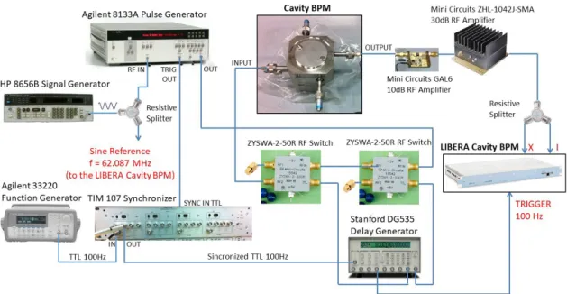
5.1 _{Test-stand at LNF-INFN}

The validation and the first measurements on the Cavity BPMs and their read-out electronics (the “LIBERA CavityBPM” module) were performed in the SELCED (“Servizio Elettronica, Controlli e Diagnostica”) laboratory at INFN-LNF. The first goal for this session of measurements was to test all the functionalities of the “LIBERA Cavity BPM” modules, as the last phase of the development process, that was carried on in collaboration with the Instrumentation Technologies staff. The second goal was to perform measurements on the Cavity BPMs and the readout electronics, characterizing their features and performances as a single measuring system. In order to achieve both goals, we developed a test-stand that includes one cBPM and one “LIBERA for CavityBPM” module. The idea was to develop a system capable to “simulate” the passage of a beam through the cBPM as the one expected at ELI-NP GBS linac [40]. The latter, in multi-bunch operation mode (see section 1.2), is composed by trains of 32 bunches, with a repetition rate of 100 Hz and a time interval between bunches of 16.1 ns.

The setup is developed on the idea of using one cBPM as a filter for a train of pulses generated in laboratory. This was possible because the “position” resonator of the cBPM (model PSI Cavity BPM16, see Figure 3.6) has two ports for the horizontal axes and two for the vertical axes. As such, we used one port (on the horizontal axes) as the input port to excite the “position” resonator and the other horizontal port as the output one.

In order to reconstruct the position of the beam on one axes, the read-out electronics needs the signal from the “position” resonator of that axes (Channel “X” or “Y”) and the signal from the “reference” resonator (Channel “I”). With the test-stand used, it is not possible to use the “reference” resonator of the cBPM, as there is only one port associated to it. Thus, in order to provide a signal on channel “I”, we split the signal (by means of a balanced resistive splitter) at the port used as the output of the cBPM. As such, half of the signal is provided at channel “X” and half at channel “I”. This work around is based on the fact that the resonance frequency of the position resonator and reference resonators of the cBPM have roughly the same frequency and quality factor (see Table 3.2). It also has another benefit: since the position calculation is based on the ratio of the amplitudes on channel “X” and channel “I”, by using only one cBPM output signal, split in two halves, the noise associated to the input signal and injected into the

(43)

42

front-end of the readout electronics is greatly reduced, similarly to the case of measuring a noisy signal in differential mode.

The general layout of the test-stand is shown in Figure 5.1.

Figure 5.1: Layout of the test-stand used in laboratory at LNF, by using cBPM output signals. Courtesy of Donato Pellegrini.

The Pulse Generator “Agilent 8133A” is used to generate pulses of 2 V with a width of 50 ps and a time interval between them of 16.1 ns, corresponding to a repetition frequency of 62.087 MHz. This signal is gated by means of a cascade of two switches “ZYSWA-2 50R” with the output signal of the Delay Generator “Stanford DG535”. The latter provide a variable gate window which could be regulated to overlap in time with a variable number of consecutive bunches, with a repetition rate of 100 Hz. For example, by adjusting its time length to roughly 512 ns, it is possible to allow the passage of 32 consecutive bunches through the switches. The train of pulses is then provided to one of the port of the “position” resonator of the cBPM. The reason to uses two switches in cascade instead of one is to increase the input-output isolation. Due to impedance miss-matching between the RF-switches and the cavity port used as the input port, we detected the effects of unwanted signal reflections on the output signal of the cBPM. These reflections were reduced by installing a 50 Ω - 3dB attenuator at the cBPM input port (not depicted in Figure 5.1). At the other port of the cBPM (used as the output port), two amplifiers are installed (Mini Circuits “GAL6” and Mini Circuits “ZHL-1042J-SMA”)

(44)

43

for a total nominal gain of 40 dB. The amplified signal is then provided to the channel “X” and channel “I” of the “LIBERA for Cavity BPM”, by means of a resistive splitter.

The reference signal at 62.087 MHz is provided to the “LIBERA for Cavity BPM” by the Signal Generator “HP 8656B”. The latter is used also as the input trigger of the Pulse generator, in order to guarantee that the reference signal is synchronized with the train of pulses. The trigger at 100 Hz is provided by the “Stanford DG535” delay generator. Since the trigger and the train of pulses are generated by different devices, synchronization of the two signals is required. In order to achieve this, a Synchronizer device (“TIM 107”) is used. It synchronizes two signals: the output trigger of the pulse generator (at a frequency of 62.087 MHz), synchronous with the generation of pulses; the TTL square wave with a frequency of 100 Hz, provided by the function generator “Agilent 33220”. Thus, the output of the Synchronizer is a signal with a frequency of 100 Hz, whose rising edges are synchronized with the pulses generated by the pulse generator. This signal is provided to the Delay Generator, which is, as already explained, used to gate the train of pulses and to provide the trigger to the “LIBERA for CavityBPM”.

The cBPM output signals produced by the test-stand are shown in Figure 5.2 and Figure 5.3, for the case of single pulse excitation and 32-pulses excitation. We detected high levels of distortion on the signal spectrum, introduced by the two amplifiers installed at the output port of the cBPM. As such, most of the measurements performed with this setup and presented here were performed without them.

(45)

44

Figure 5.3: Magenta waveform: cBPM output signal with a train of 32 pulses excitation (amplified). Green waveform: sine reference at 62.087 MHz. Yellow waveform: signal used for the gating of the train of pulses.

The amplitude of the signal after the resistive splitter and without the amplifiers has a maximum amplitude of ~ 17 mV, sufficient to reach about ±2000 counts of the ADC used by the “LIBERA Cavity BPM”, out of its maximum range of -8191/+8192 counts.

5.1.1 Test-stand at LNF-INFN with sinewave signals

Some of the measurements were performed by using sinewave signals at a frequency of 3.284 GHz (the same value of the resonance frequency of the cBPM). In this case the test-stand used is shown in Figure 5.4. We used a Vector Analyzer (AGILENT E5071B) to produce a sinewave signal at 3.284 GHz. As in the previous case, the signal is split and provided to channel “X” and “I” of the readout electronics. The trigger is provided by the Delay Generator (STANFORD DG535), while the reference signal at 62.087 MHz is provided by the signal generator “HP 8656B”. Since we used a continuous waveform, there was no need to synchronize the signal with the reference or the trigger.

Studies and measurements on cavity beam position monitors for novel electron linacs

Department of Physics

Accelerator Physics PhD School – XXXII cycle

Studies and Measurements on

Cavity Beam Position Monitors

for Novel Electron Linacs

Giovanni Franzini

Director of Doctoral School:

Supervisor:

Prof. Daniele Del Re

Prof. Luigi Palumbo

Co-supervisor:

Prof. Andrea Mostacci

Studies and Measurements on Cavity Beam

Position Monitors for Novel Electron Linacs

G. Franzini

Contents

Introduction

Dissertation overview

1

Extreme Light Infrastructure – Nuclear

Physics – Gamma Beam System

1.1

Interaction points and Cavity BPMs

1.2

ELI-NP-GBS LINAC overview

2

Diagnostics for ELI-NP GBS

2.1

Overview

2.2

Beam Charge Monitors

2.3

Stripline Beam Position Monitors

2.4

Cavity Beam Position Monitors

3

Cavity Beam Position Monitors

3.1

Theory and Working principle

3.2

Cavity Beam Position Monitors for ELI-NP GBS

4

Readout Electronics for Cavity BPM

4.1

Front end electronics and digitizer

4.1.1

Variable attenuators

4.1.2

Down conversion and digitization

4.2

Digital processing

4.2.1

Calculation of the beam position

4.2.2

Deconvolution filter (for multi-bunch operation)

5

Bench measurements on Cavity BPM

5.1

Test-stand at LNF-INFN

5.1.1

Test-stand at LNF-INFN with sinewave signals

_{Interaction points and Cavity BPMs}

_{ELI-NP-GBS LINAC overview}

_{Stripline Beam Position Monitors}

_{Theory and Working principle}

_{Cavity Beam Position Monitors for ELI-NP GBS}

_{Test-stand at LNF-INFN}