The Synchronized Location-Transshipment Problem

(1)

ScienceDirect

Transportation Research Procedia 52 (2021) 43–50

This is an open access article under the CC BY-NC-ND license (https://creativecommons.org/licenses/by-nc-nd/4.0) Peer-review under responsibility of the scientific committee of the 23rd Euro Working Group on Transportation Meeting 10.1016/j.trpro.2021.01.007

10.1016/j.trpro.2021.01.007 2352-1465

This is an open access article under the CC BY-NC-ND license (https://creativecommons.org/licenses/by-nc-nd/4.0) Peer-review under responsibility of the scientific committee of the 23rd Euro Working Group on Transportation Meeting

Transportation Research Procedia 00 (2020) 000–000 _{www.elsevier.com/locate/procedia}

23rd EURO Working Group on Transportation Meeting, EWGT 2020, 16-18 September 2020,

Paphos, Cyprus

The Synchronized Location-Transshipment Problem

Teodor Gabriel Crainic

a,b

_{, Riccardo Giusti}

c

_{, Daniele Manerba}

d,∗

_{, Roberto Tadei}

c

a_{School of Management Sciences, Université du Québec à Montréal, Montréal (Canada)} b_{CIRRELT, Montréal (Canada)}

c_{Department of Control and Computer Engineering, Politecnico di Torino, Turin (Italy)} d_{Department of Information Engineering, Universit`a degli Studi di Brescia, Brescia (Italy)}

Abstract

To improve efficiency and sustainability in synchromodal logistics, it becomes crucial to mitigate the disruptive effects caused by non-synchronized operations. In this work, we study the Synchronized Location-Transshipment Problem in which the decisions on the facilities to select are fundamental to ensure the synchronization of flows and the correct exploiting of just-in-time logistics and cross-docking operations. We propose a Mixed-Integer Linear Programming formulation for the problem and perform an economic analysis to address several realistic situations based on different sizes of the transshipment facilities and location types. The results of the tests allow us to derive managerial insights and to define future research lines.

Peer-review under responsibility of the scientific committee of the 23rd EURO Working Group on Transportation Meeting..

Keywords: Synchromodal Logistics; Location-Transshipment; Cross-Docking.

1. Introduction

The primary purpose of synchromodal logistics is to improve the quality and the sustainability of the services while reducing costs by enhancing the vertical and horizontal cooperation among stakeholders. This improvement is made by providing relevant real-time information to all parties and adopting the most flexible door-to-door shipments. Those characteristics allow a better synchronization of the operations to be adopted. Moreover, proper synchronization is required to implement procedures based on the just-in-time and cross-docking paradigms. The former asks that every shipment should arrive only when it is needed to avoid storage costs and unmet demand. At the same time, the latter consists of transshipping goods as fast as possible through intermediate hubs. Finally, synchromodality has been linked to physical internet, and the two paradigms can benefit one from the other (Ambra et al.,2019).

Implementing a perfect synchronization requires that someone takes the role of an orchestrator to coordinate all stakeholders. The orchestrator, which can be identified as a Logistics Service Provider (LSP), should be capable

∗_{Corresponding author. Tel.: +39 030 371 5935.}

E-mail address: daniele.manerba@unibs.it

Transportation Research Procedia 00 (2020) 000–000 _{www.elsevier.com/locate/procedia}

23rd EURO Working Group on Transportation Meeting, EWGT 2020, 16-18 September 2020,

Paphos, Cyprus

The Synchronized Location-Transshipment Problem

Teodor Gabriel Crainic

a,b

_{, Riccardo Giusti}

c

_{, Daniele Manerba}

d,∗

_{, Roberto Tadei}

c

a_{School of Management Sciences, Université du Québec à Montréal, Montréal (Canada)} b_{CIRRELT, Montréal (Canada)}

c_{Department of Control and Computer Engineering, Politecnico di Torino, Turin (Italy)} d_{Department of Information Engineering, Universit`a degli Studi di Brescia, Brescia (Italy)}

Abstract

To improve efficiency and sustainability in synchromodal logistics, it becomes crucial to mitigate the disruptive effects caused by non-synchronized operations. In this work, we study the Synchronized Location-Transshipment Problem in which the decisions on the facilities to select are fundamental to ensure the synchronization of flows and the correct exploiting of just-in-time logistics and cross-docking operations. We propose a Mixed-Integer Linear Programming formulation for the problem and perform an economic analysis to address several realistic situations based on different sizes of the transshipment facilities and location types. The results of the tests allow us to derive managerial insights and to define future research lines.

Keywords: Synchromodal Logistics; Location-Transshipment; Cross-Docking.

1. Introduction

The primary purpose of synchromodal logistics is to improve the quality and the sustainability of the services while reducing costs by enhancing the vertical and horizontal cooperation among stakeholders. This improvement is made by providing relevant real-time information to all parties and adopting the most flexible door-to-door shipments. Those characteristics allow a better synchronization of the operations to be adopted. Moreover, proper synchronization is required to implement procedures based on the just-in-time and cross-docking paradigms. The former asks that every shipment should arrive only when it is needed to avoid storage costs and unmet demand. At the same time, the latter consists of transshipping goods as fast as possible through intermediate hubs. Finally, synchromodality has been linked to physical internet, and the two paradigms can benefit one from the other (Ambra et al.,2019).

Implementing a perfect synchronization requires that someone takes the role of an orchestrator to coordinate all stakeholders. The orchestrator, which can be identified as a Logistics Service Provider (LSP), should be capable

∗_{Corresponding author. Tel.: +39 030 371 5935.}

E-mail address: daniele.manerba@unibs.it

(2)

44 Teodor Gabriel Crainic et al. / Transportation Research Procedia 52 (2021) 43–50

2 Crainic et al. / Transportation Research Procedia 00 (2020) 000–000

in particular of implementing sophisticated planning, which has been identified as a critical success factor for the realization of synchromodality (Pfoser et al.,2016). The European Commission has recognized the importance of Synchromodality by founding Horizon2020 projects on this topic (Giusti et al.,2018, 2019a) but still few works have appeared, especially from a quantitative perspective and regarding strategic planning (Giusti et al.,2019b). This type of planning implies long-term decisions that will affect the performance of logistic networks for a long time in the future. Hence, it is crucial to make the right decisions to set up the base to achieve a proper synchronization of the operations with the relative benefits. Given the lack of literature and the new features that must be considered to implement a synchromodal logistics network, we decided to study the Synchronized Location-Transshipment Problem (SLTP), which involves decisions about locating facilities where to do transshipment operations.

Since in the literature there are lacks about Location-Transshipment problems in synchromodal logistics, in our attempt to deal with this problem, we simplify some aspects that we will consider in future works (see Section3and

7for more details). Then, our work aims at presenting a Mixed-Integer Linear Programming (MILP) formulation for the SLTP considered in the context of synchromodality. In our experimental setting, we will solve ten instances for eight different test-cases, in which both the size and the type of transaction needed to secure the facilities differ. Then, we will analyze and discuss the results to provide useful managerial insights. Our objective is to understand better how the selection of different types of facilities has an impact on costs.

The rest of the paper is organized as follows. In Section2, we discuss the literature review relevant to the prob-lem. In Section3, we describe the logistics setting and the problem that we want to study. Then, the derived model is presented in Section4. Section5 discusses the experimental setting and Section6 the results obtained. Finally, conclusions and future research lines are presented in Section7.

2. Literature review

The SLTP comprises strategic planning about locating transshipment facilities but, to make the best decisions, the utilization of the resulting structure must also be considered. This can be done by merely allocating customers to facilities or by a more detailed representation of the operations, that can involve the management of flows and shipments. For instance, the allocation of flows throughout networks with transshipment facilities are studied byBaldi et al.(2012) to minimize the total costs andTadei et al.(2012) to maximize the total net utility, whereasMar´ın(2011) deals with the assignment of customers to potential plants.

In the SLTP within the synchromodal logistics paradigm, it is even more important to look at the operational level while designing a network that should be capable of allowing an optimal synchronization of operations (Giusti et al.,

2020). Moreover, adopting flexible synchromodal policies instead of rigid ones provides better results and decreases the impact of overloading transshipment facilities, by mitigating delays propagation with flow synchronization (Qu et al., 2019). The benefits of synchronization have been pointed out many times in literature, for instance, by Jin et al.(2018) that designed services to move containers between neighboring local ports synchronized with long-haul services orLuo et al.(2019) that considered cross-docking procedures and synchronization between production and warehouse operations. Instead,Neves-Moreira et al.(2016) synchronized short-haul jobs of trucks, that can exchange semi-trailers to provide long-haul services, to reduce empty truck journeys.

Very often, the location of intermediate facilities is a crucial decision, involving in many cases huge investments, especially when global or inter-continental logistics networks are considered. For instance,Zhao et al.(2018) studied the crucial problem of locating consolidation centers under the One Belt One Road initiative, with which China aims to improve the efficiency of their international transportation system. Due to the impact of location decisions and the lack in the literature regarding the SLTP problem in synchromodal logistics, we decided to define a variant of the problem that considers the flow synchronization issue.

3. Logistics setting and problem description

We consider the problem of an LSP that needs to manage a network with different origins (e.g., production plants, distribution centers) that supply freight to fulfill the demand at different destinations (e.g., distribution centers, cus-tomers, retailers). The LSP treats single-commodity flows, i.e., only one type of demand for all the destinations and

(3)

the same type for the supply in all the origins. This structure usually represents logistics networks in which indistin-guishable products (e.g., oil) are shipped.

To improve the efficiency of the transport network, all the freight from any origin to any destination passes by intermediate transshipment facilities in which a certain number of handling operations are performed. Each facility has a maximum handling capacity (equal in each period) and, to be located, facilities should also satisfy a minimum requirement about their utilization over the whole optimization horizon. Then, the strategic decision that the LSP needs to take is which transshipment facilities should locate, and their utilization considering the operational decision on how allocating the freight flows through them.

Moreover, to meet the requirement of just-in-time and cross-docking procedures, the LSP should synchronize the flows to avoid leftovers at the facilities and to fulfill the demand exactly when it is needed at the destinations. Note that the supply is collected and sent through the network as soon as it is ready but, due to possible disruptions and lack of synchronization of the flows, freight may arrive earlier or later than expected. Both events cause additional costs. The first because of storage needed at the destinations. The second because of dissatisfaction with the demand in time. Note that, however, we will always talk about earliness penalties instead of storage costs at destinations in order not to confuse them with storage costs at facilities.

4. Mixed-Integer Linear Programming formulation

To model the above setting, we introduce a deterministic and multi-period Synchronized Location-Transshipment Problem (SLTP) in which synchronization procedures are addressed to reduce the overall cost of the network. We decided to model the decision problem through a multi-period setting that considers storage costs, earliness penalties, and lateness penalties to represent better synchronization mechanisms, that are essential to implement synchromodal, just-in-time, and cross-docking procedures. The model aims to locate the set of transshipment facilities that can guarantee an optimal flow synchronization to avoid the most leftovers and penalties.

Let us consider the following sets • I: set of origins;

• J: set of destinations; • K: set of facilities;

• T = {0, 1, 2, . . . , tmax}: ordered set of periods (e.g., a day) representing the optimization horizon (e.g., a month);

and the following parameters • pt

i: supply of freight units in an origin i ∈ I in a time period t ∈ T;

• qt

j: demand of freight unit in a destination j ∈ J in a time period t ∈ T;

• C+

k: maximum handling capacity of a facility k ∈ K available in each time period t ∈ T;

• C−

k: minimum handling capacity that should be used in a facility k ∈ K over the whole optimization horizon |T|;

• τik≥ 1 and δk j≥ 1: discrete travelling time (i.e., number of time periods) needed to move freight from an origin

i ∈ I to a facility k ∈ K and from a facility k ∈ K to a destination j ∈ J, respectively;

• fk: cost of locating a facility k ∈ K;

• ht

k: cost of handling freight in a facility k ∈ K in a period t ∈ T;

• cikand gk j: cost of transportation for a freight unit from an origin i ∈ I to a facility k ∈ K and from a facility

k ∈ K to a destination j ∈ J, respectively;

• dt

k: cost of storing a freight unit in a facility k ∈ K in a period t ∈ T;

• at

j: cost of storing a freight unit in a destination j ∈ J in a period t ∈ T (cost of earliness);

• bt

j: cost of the unmet demand of freight units at a destination j ∈ J in a period t ∈ T (cost of lateness).

We assume that _i∈I_t∈Tpt

i =j∈Jt∈Tqti, i.e., the system is balanced and the total supply is always equal to the

total demand.

(4)

• xk∈ {0, 1}: binary variables equal to 1 if a facility k ∈ K is located;

• yt

k∈ [0, 1]: continuous variables representing the percentage of the whole capacity used to handling freight of a

facility k ∈ K in a period t ∈ T; • zt

ik≥ 0 and vtk j ≥ 0: continuous variables representing the freight units departing in a period t ∈ T from an origin

i ∈ I to a facility k ∈ K and from a facility k ∈ K to a destination j ∈ J, respectively;

• wt

k≥ 0: continuous variables representing the freight units at a facility k ∈ K in a time period t ∈ T. We use this

variable to keep track of leftovers; • et

j≥ 0: continuous variables representing the amount of freight units arrived too early that need to be stored in

a destination j ∈ J in a time period t ∈ T; • lt

j≥ 0: continuous variables representing the amount of unsatisfied demand of freight units in a destination j ∈ J

in a time period t ∈ T.

Then, a Mixed-Integer Linear Programming formulation for the problem is as follows: min x,y,z,v,w,e,l k∈K fkxk+ k∈K t∈T ht kytk+ k∈K t∈T    i∈I cikztik+ j∈J gk jvtk j    + + k∈K t∈T dt k   wtk− j∈J vt k j    + j∈J t∈T at jetj+ j∈J t∈T bt jltj (1) subject to yt k≤ xk, k ∈ K, t ∈ T (2) k∈K zt ik=pti, i ∈ I, t ∈ T (3) k∈K t∈T | t≥δk j v(t−δk j) k j = t∈T qt j, j ∈ J (4) t∈T C+ k ytk≥ C−k xk, k ∈ K (5) j∈J vt k j≤ C+k ytk, k ∈ K, t ∈ T (6) j∈J vt k j≤ wtk, k ∈ K, t ∈ T (7) w0 k=0, k ∈ K (8) wt k=w(t−1)k − j∈J v(t−1)_{k j} + i∈I | t≥τik z(t−τik) ik , k ∈ K, t ∈ {1, 2, . . . , tmax} (9) e0 j,l0j=0, j ∈ J (10) k∈K | t≥δk j v(t−δk j) k j − etj+ltj+e(t−1)j − l(t−1)j =qtj, j ∈ J, t ∈ {1, 2, . . . , tmax} (11) xk∈ {0, 1}, k ∈ K (12) yt k≥ 0, k ∈ K, t ∈ T (13) zt ik≥ 0, i ∈ I, k ∈ K, t ∈ T (14) vt k j≥ 0, k ∈ K, j ∈ J, t ∈ T (15) wt k≥ 0, k ∈ K, t ∈ T (16) et j,ltj≥ 0, j ∈ J, t ∈ T. (17)

(5)

The objective function (1) aims at minimizing the total cost of the logistics network. Here, the first term represents location costs F(x), the second terms handling costs H(y), the third transportation costs T(z, v) , the fourth storage costs S (w, v), the fifth earliness penalties E(e), and the sixth lateness penalties L(l). Constraints (2) ensure that a facility is used only if it is located. Constraints (3) force to collect the supply immediately in all origins in each period, whereas constraints (4) ensure that the total demand of a destination is satisfied over the whole optimization horizon. Constraints (5) guarantee a minimum utilization of the located facilities over the whole optimization horizon. Instead, constraints (6) and (7) limit the amount of freight that can be handled to the available handling capacity, and the available units of freight at any facility in each period, respectively. The freight that needs to be handled in a facility is defined by constraints (8) and (9). In the first period, we have zero units of freight at each facility, whereas in the following periods, leftovers must be handled together with the new arrivals. Constraints (10) represent the initial earliness and lateness that are updated by constraints (11) depending on the previous values assumed, the new arrivals, and the current demand at a destination. Finally, constraints (12)–(17) are simple conditions on variables.

5. Experimental settings

We perform an economic analysis by considering different sizes of the facilities, namely, small (S), medium (M), and large (L), and different types of transactions needed to secure them, i.e., a buy (B) or a temporary contract (C). The aim is to evaluate the impact of such features on the objective function and the different costs. Depending on the size, facilities have different handling capacities, and their handling costs also vary. We consider that small facilities have less equipment than large ones, implying less efficiency to perform the handling operations. For the location types, instead, we consider that a facility has higher handling costs if located since an extra cost is required to delegate the handling operations. Note that we consider the same contract cost for facilities that can be bought (type B) or that can only be contracted (type C) since both require high investments on very long periods. In this analysis, we are interested in the impact of their utilization costs on the overall cost of the whole transport network.

For the tests, we generate ten instances with different random seeds and with a number of origins |I| = 10, number of destinations |J| = 40, and number of time periods |T| = 31. To better approximate a realistic structure of the network, we also define origins with different amount of supplies and destinations with different amount of demands. Hence, we subdivide the set of origins I into origins with low (|Ilow| = 0.6|I|), medium (|Imed| = 0.3|I|), and high

(|Ihigh| = 0.1|I|) supply. Instead, the set of destinations J is subdivided into destinations with low (|Jlow| = 0.25|J|),

medium (|Jmed| = 0.5|J|), and high (|Jhigh| = 0.25|J|) demands. Since the total capacity is related to the total demand

of the network, the number of facilities |K| can differ in each instance. Moreover, the possible different sizes of the facilities are another factor that can increase or decrease the number of facilities. Depending on their size, facilities can have different handling costs. Furthermore, the types of facilities B and C imply different economies of scale. We test each instance over eight different test cases in which we consider all the six combinations of size (S, M, and L) and location type (B and C) and the other two cases in which we have all the different size types considered at once (SML). We use the following notation to discuss the eight test cases: S-B, M-B, L-B, SML-B, S-C, M-C, L-C, and SML-C.

The generation of the instances is done by adopting reasonable realistic values for the main problem parameters, calculated as the percentage of destinations for each size of demand and the percentage of origins for each size of supply. Moreover, we keep a proportion between those parameters and the others in order to make the instance generation procedure scalable for networks with different sizes. In detail, the parameters are generated as follows:

• we compute the total demand qtot=|T| (15 |Jlow| + 60 |Jmed| + 160 |Jhigh|);

• the flow demand qt

j, for each t ∈ T, is drawn from U[5, 25] for each j ∈ Jlow, from U[40, 80] for each j ∈ Jmed,

and from U[120, 200] for each j ∈ Jhigh. Note that, we further adjust the demands to always guarantee that

j∈Jt∈Tqtj=qtot;

• the flow supply pt

i, for each t ∈ T, is drawn from U[0.8 ¯psize,1.2 ¯psize] with psizedifferent for each i ∈ Ilow, for

each i ∈ Imed, and for each i ∈ Ihigh, where ¯psize= qtot

3 |Isize| |T|for each different size. Note that, we further adjust

the supplies to always guarantee that _i∈I_t∈Tpt

(6)

• the handling capacity C+

k, for each k ∈ K, is equal to 50 for small-sized, 200 for medium-sized, and 500 for

large-sized facilities. Then, the number of facility |K| for each test case is about _{|T| C}2 qtot

size, where with Csizewe

mean the handling capacity C+

k for the different size-cases. For the test case SML, we split the total demand qtot

in three and then we use the same logic as before;

• the minimum handling capacity over the whole time horizon C−

k, for each k ∈ K, is equal to 0.5t∈TC+k;

• the travel time τik, for each i ∈ I, k ∈ K, and the travel time δk j, for each k ∈ K, j ∈ J, are drawn from

U[0.1|T|, 0.2|T|]. Note that, the bounds are rounded to the nearest integer and all the parameters are set to 1 every time a zero is drawn;

• the unitary travel costs cik, for each i ∈ I, k ∈ K, and gk j, for each k ∈ K, j ∈ J, are respectively equal to 0.02τik

and 0.02δk j;

• the cost of locating a facility fk, for each k ∈ K, is equal to 10 Ck;

• the cost of using a facility ht

k, for each k ∈ K, t ∈ T, is equal to 0.1 δ Ck, where δ is a parameter which depends

on the type of the facility;

• the cost of storing a freight unit in a facility dt

k, for each k ∈ K, t ∈ T, is equal to 0.2 htk;

• the cost of storing a freight unit in a destination at

j, for each j ∈ J, t ∈ T, is equal to

0.2 _k∈K_t∈Tht k

|K| |T| ;

• the cost of unmet demand of a freight unit bt

j, for each j ∈ J, t ∈ T, is equal to 1.5 atj.

Lastly, to ensure that the initial demand can be fulfilled and that the last demand can have lateness, we consider a larger optimization horizon. In practice, the supply starts in period 0, and it finishes in period T, whereas the demand starts after 0.3 |T| periods, and it ends after 1.3 |T| periods. An additional 0.3 |T| periods are left after the end of the demand to make it also possible to fulfill the last demand with lateness penalties. The periods in which there are positive supply and demand are equal to |T|.

To solve the instances, we input the relative MILP model into the CPLEX solver v12.9 (IBM ILOG CPLEX,2019) via its Java Concert Technology APIs. Moreover, to avoid CPLEX to get stuck too long around an almost optimal solution, we set a MIP gap of 2%. Computational experiments have been done on an Intel(R) Core(TM) i7-7560U CPU@2.40 GHz machine with 16 GB RAM and running Windows 10 Pro 64-bit operating system.

6. Results and discussion

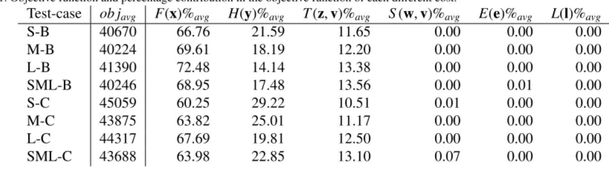
We want to analyze for all the test cases the variation of costs, number of facilities located, and capacity utilization. Costs are presented in Table (1), whereas the number of facility located and the capacity utilization is given in Table (2). In both tables, we have eight rows in which each value represents the average value over all the ten instances for each test case. Then, in Table (1) we present the objective function (ob javg) and the percentage contribution of

each cost to the objective function (F(x)%avg, H(y)%avg, T(z, v)%avg, S (w, v)%avg, E(e)%avg, and L(l)%avg). Instead

in Table (2), for each type of size we present the percentage of facilities located with respect to the total number (locS %avg, locM%avg, and locL%avg) of that type, and the utilization percentage in terms of total capacity of the

located facilities (usageS %avg, usageM%avg, and usageL%avg). Note that, we do not report the standard deviation

of the obtained values since they are quite low and, therefore, we can consider stable the average values. Regarding computation times, on average it needs between 30 and 226 seconds to solve the model, but without the MIP gap of 2% the solving time increases dramatically.

In terms of the objective function (Table1), the test case SML and M have similar values and are better when compared with the other cases with the same location type, having the best balance between location and handling costs. Instead, case L-B has higher costs respect to the case S-B, whereas it is the opposite if we consider case S-C and L-C. Lastly, comparing the objective functions of the location type B and C gives useful insights into how much we should invest in contract facilities instead of buying them. Since this trade-off shows that buying a large facility will require longer to repay the investment, it could be more convenient to buy small facilities and contract large ones. We can notice that the cost contributions derived by storage S (w, v), earliness E(e), and lateness L(l) are always very close to 0. Even if supplies and demands in each period are different for each instance, by solving the model, it is always possible to synchronize the flows to avoid almost all of the above cost contributions. Hence, it does not matter

(7)

Table 1. Objective function and percentage contribution in the objective function of each different cost.

Test-case ob javg F(x)%avg H(y)%avg T(z, v)%avg S (w, v)%avg E(e)%avg L(l)%avg

S-B 40670 66.76 21.59 11.65 0.00 0.00 0.00 M-B 40224 69.61 18.19 12.20 0.00 0.00 0.00 L-B 41390 72.48 14.14 13.38 0.00 0.00 0.00 SML-B 40246 68.95 17.48 13.56 0.00 0.01 0.00 S-C 45059 60.25 29.22 10.51 0.01 0.00 0.00 M-C 43875 63.82 25.01 11.17 0.00 0.00 0.00 L-C 44317 67.69 19.81 12.50 0.00 0.00 0.00 SML-C 43688 63.98 22.85 13.10 0.07 0.00 0.00

Table 2. Location percentage respect to the total number of facilities per type and percentage utilization in terms of capacity of the located facilities for each size.

Test-case locS %avg locM%avg locL%avg usageS %avg usageM%avg usageL%avg

S-B 46.02 0.00 0.00 70.18 0.00 0.00 M-B 0.00 48.28 0.00 0.00 68.04 0.00 L-B 0.00 0.00 54.55 0.00 0.00 63.51 SML-B 28.46 62.22 73.34 69.11 68.66 68.27 S-C 46.02 0.00 0.00 70.18 0.00 0.00 M-C 0.00 48.28 0.00 0.00 68.04 0.00 L-C 0.00 0.00 54.55 0.00 0.00 63.51 SML-C 9.49 64.45 96.67 68.19 68.19 68.09

which facilities we are using if we can predict supplies and demand perfectly, but having the right amount of capacity is already enough. This scenario may drastically change in a stochastic environment, which will be the subject of our future studies.

Regarding transportation costs T(z, v) instead, it seems that the size of the facilities considered affects them. Prob-ably, this happens because a higher number of facilities (type S) allows reducing the total transportation cost. We can deduce that by locating a higher amount of facilities, the flow can be better allocated to avoid transportation costs. Location costs F(x) increase with the size of the facilities considered. In the test case SML, they are close to those of the test case M. Instead, the handling costs H(y) tend to decrease with the size. This means that if we plan to use a facility for a long time, it will cost more in terms of location costs, but the cheaper costs of the handling operations, especially in the cases B, will ensure a higher return of investment.

From the percentage of located facilities in Table2), we can notice that fewer facilities out of the total number are needed for a smaller size. Instead, in SML, a great percentage of large facilities (almost all for the test case SML-C) are used together with a significant part of the medium facilities. Small facilities, especially for the test case SML-C, are few compared to the total. The combination of their location and handling costs makes them quite expensive and inconvenient.

Finally, note that, in the test-case SML, the percentage of facility utilization is more or less the same for all sizes. Instead, in other cases, the utilization decrease if the size increase, showing that small facilities tend to have a higher usage level. This is perfectly reasonable if the demand is known precisely, and there are no disruptions on our logistics network. In reality, having some unused capacity will allow tackling those drawbacks

7. Conclusions

We presented a MILP formulation for the single-commodity multi-period Synchronized Location-Transshipment Problem, to perform the first study of a realistic setting in the context of synchromodal logistics. In particular, we addressed the precise fulfillment of the demand required for the just-in-time paradigm and the need to avoid leftovers as much as possible for the cross-docking paradigm. Moreover, we presented an economic analysis based on the proposed model to study different test-cases and derived managerial insights.

(8)

The trade-off between the objective functions of the different test-cases shows that it can be more convenient to buy small facilities and to contract large ones. Instead, if we plan investment for a very long period, buy a large facility grant the higher return of investment. Regarding transportation costs, having a higher number of facilities can help to decrease these costs. Furthermore, the results show that a network that comprises medium-size facilities or facilities with different sizes performs better in terms of minimization of the costs. Lastly, the tests proved that, in a deterministic environment, the model could synchronize the flows optimally to avoid almost all costs and penalties derived by leftovers, earliness, and lateness.

Future improvements will consist of adding to the model multi-commodity flows, representing different customers and products. Furthermore, it would be interesting to consider some source of uncertainty (e.g., on supply and demand) and compare the performance in terms of the optimal solutions of the deterministic model presented in the paper with the new stochastic ones. Since the deterministic solutions already know exactly demands and supplies, the model is capable of synchronizing the flows almost entirely. Still, it could activate storage costs and earliness/lateness penalties if the plan about locating and handling operations are executed as they are in a stochastic environment. These two improvements will be significant to make the synchronization even more meaningful and fit better this problem in the context of synchromodal logistics.

References

Ambra, T., Caris, A., Macharis, C., 2019. Towards freight transport system unification: reviewing and combining the advancements in the physical internet and synchromodal transport research. International Journal of Production Research 57, 1606–1623. doi:10.1080/00207543. 2018.1494392.

Baldi, M.M., Ghirardi, M., Perboli, G., Tadei, R., 2012. The capacitated transshipment location problem under uncertainty: A computational study. Procedia - Social and Behavioral Sciences 39, 424 – 436. doi:10.1016/j.sbspro.2012.03.119.

Giusti, R., Iorfida, C., Li, Y., Manerba, D., Musso, S., Perboli, G., Tadei, R., Yuan, S., 2019a. Sustainable and de-stressed international supply-chains through the synchro-net approach. Sustainability 11, 1083. doi:10.3390/su11041083.

Giusti, R., Manerba, D., Bruno, G., Tadei, R., 2019b. Synchromodal logistics: An overview of critical success factors, enabling technologies, and open research issues. Transportation Research Part E: Logistics and Transportation Review 129, 92–110. doi:10.1016/j.tre.2019. 07.009.

Giusti, R., Manerba, D., Perboli, G., Tadei, R., Yuan, S., 2018. A new open-source system for strategic freight logistics planning: The SYNCHRO-NET optimization tools. Transportation Research Procedia 30, 245–254.

Giusti, R., Manerba, D., Tadei, R., 2020. Multi-period transshipment location-allocation problem with stochastic synchronized operations. Networks (to appear).

IBM ILOG CPLEX, 2019. IBM ILOG CPLEX Optimization Studio V12.9.0 documentation. https://www.ibm.com/support/

knowledgecenter/en/SSSA5P_12.9.0/ilog.odms.studio.help/Optimization_Studio/topics/COS_home.html. Accessed:

2020-07-25.

Jin, J.G., Meng, Q., Wang, H., 2018. Column generation approach for feeder vessel routing and synchronization at a congested transshipment port, in: Proceedings of Odysseus 2018 - 7th International Workshop on Freight Transportation and Logistics, June 3-8, 2018, Cagliari (Italy). Luo, H., Yang, X., Wang, K., 2019. Synchronized scheduling of make to order plant and cross-docking warehouse. Computers & Industrial Engineering 138, 106108. doi:10.1016/j.cie.2019.106108.

Mar´ın, A., 2011. The discrete facility location problem with balanced allocation of customers. European Journal of Operational Research 210, 27–38. doi:10.1016/j.ejor.2010.10.012.

Neves-Moreira, F., Amorim, P., Guimar˜aes, L., Almada-Lobo, B., 2016. A long-haul freight transportation problem: Synchronizing resources to deliver requests passing through multiple transshipment locations. European Journal of Operational Research 248, 487–506. doi:10.1016/ j.ejor.2015.07.046.

Pfoser, S., Treiblmaier, H., Schauer, O., 2016. Critical success factors of synchromodality: Results from a case study and literature review. Transportation Research Procedia 14, 1463–1471.

Qu, W., Rezaei, J., Maknoon, Y., Tavasszy, L., 2019. Hinterland freight transportation replanning model under the framework of synchro-modality. Transportation Research Part E: Logistics and Transportation Review 131, 308–328. doi:10.1016/j.tre.2019.09.014. Tadei, R., Perboli, G., Ricciardi, N., Baldi, M.M., 2012. The capacitated transshipment location problem with stochastic handling utilities at the facilities. International Transactions in Operational Research 19, 789–807. doi:10.1111/j.1475-3995.2012.00847.x.

Zhao, L., Zhao, Y., Hu, Q., Li, H., Stoeter, J., 2018. Evaluation of consolidation center cargo capacity and loctions for China railway express. Transportation Research Part E: Logistics and Transportation Review 117, 58–81. doi:10.1016/j.tre.2017.09.007.