RICERCA DI SISTEMA ELETTRICO
Studio delle caratteristiche di impianti di illuminazione stradale
per valutare i consumi energetici e luce dispersa verso l’alto. Relazione
sintetica settembre 2012
Paolo Soardo
Report RdS/2012/085 Agenzia nazionale per le nuove tecnologie, l’energia
STUDIO DELLE CARATTERISTICHE DI IMPIANTI DI ILLUMINAZIONE STRADALE PER VALUTARE I CONSUMI ENERGETICI E LUCE DISPERSA VERSO L’ALTO. RELAZIONE SINTETICA SETTEMBRE 2012
Paolo Soardo (AIDI)
Mese e Anno: settembre 2012
Report Ricerca di Sistema Elettrico
Accordo di Programma Ministero dello Sviluppo Economico - ENEA Area: Razionalizzazione e risparmio nell'uso dell'energia elettrica
Progetto: Studi e valutazioni sull'uso razionale dell'energia: Innovazione nella illuminazione pubblica: nuove tecnologie ed integrazione smart con altre reti di servizi energetici
Pagina 3 di 25
Indice
Sommario ... 4
1 Obbiettivi del programma di ricerca ... 4
2 Aspetti psicologici ... 5
3 Compensazione della luminanza artificiale del cielo ... 5
4 Essenza del programma ... 5
5 Risultati del programma di ricerca ENEA ... 6
6 Metodologia di misura e valutazione ... 6
7 Compatibilità ambientale ... 6
8 Compatibilità energetica ... 7
9 Fattore di luminanza stradale qR (punto 1.2) ... 7
10 Confronto tra gli impianti (punto 1.1) ... 11
11 Città illuminate: sorgenti di luce diffondenti ... 13
12 Leggi regionali ... 13
13 Attività futura ... 14
Appendice A ... 15
4 Environmental compatibility ... 15
4.1 Artificial sky luminance ... 15
4.2 Star magnitude ... 15
4.3 Reduction of limiting magnitude due to artificial lighting ... 16
4.4 Detection of point-like sources: stars and luminaires ... 17
4.5 Compensation of the artificial sky luminance ... 17
Appendice B... 19
7 Environmental compatibility ... 19
8 Analysis of the territory ... 20
8.1 Sky luminance formula ... 20
8.2 Propagation of sky luminance ... 21
8.3 Weight of light sources on sky luminance ... 21
8.4 Analysis of a site ... 22
Sommario
Le misurazioni fotometriche e le simulazioni, effettuate da INRIM ed AIDI nell’ambito del programma di ricerca coordinato e finanziato dall’ENEA, dimostrano in particolare che:
le riflessioni delle superfici illuminate influiscono sulla luminanza artificiale
del cielo in misura preponderante rispetto alla luce emessa verso l’alto da apparecchi di illuminazione tecnologicamente avanzati;
l’impiego di apparecchi di illuminazione con vetro piano installati
orizzontalmente (cutoff) determina un aumento dei consumi energetici e della luminanza artificiale del cielo;
gli impianti con apparecchi dotati di vetro piano consumano il 12% circa in
più di quelli con apparecchi con vetro curvo.
La ricerca ha individuato nel fattore di luminanza stradale qR un parametro
determinante e di semplice applicazione correlabile con il flusso luminoso emesso e riflesso verso l’alto e con i consumi energetici (vedere tabella).
Riepilogo risultati relativi ad ambiente ed energia Sorg.
luce Vetro
Interdis. [m]
Illumin- [lx] Lumin. [cd/m2] Fatt. lumin. qR
misure calcoli misure calcoli misure calcoli
Ioduri piano 33,00 15 26,0 1,16 1,71 1,10 0,94
curvo 37,00 13,7 20,5 1,14 1,6 1,19 1,11
LED piano 33,00 15,8 16,7 1,4 1,1 1,27 0,94
curvo 37,00 14,7 16 1,47 1,25 1,43 1,12
La ricerca propone per il futuro nuove misurazioni e simulazioni per verificare la propagazione sul territorio degli effetti molesti dell’illuminazione stradale, anche in supporto alla definizione di prescrizioni a livello regionale e/o nazionale.
1 Obbiettivi del programma di ricerca
In fase programmatica, gli obbiettivi sono stati individuati e concordati nei seguenti quattro punti:
1.1 confrontare, a parità di caratteristiche prestazionali, l’impatto ambientale
ed energetico di diverse tipologie di impianti di illuminazione stradale;
1.2 proporre parametri per la classificazione degli impianti ai fini dei consumi
energetici e della luce dispersa verso l’alto (inquinamento luminoso) in base alla loro funzione e posizione;
1.3 proporre un algoritmo di previsione dell’impatto ambientale ed energetico
di un impianto in base alle caratteristiche quantitative prima definite;
1.4 diffondere i risultati della ricerca per valorizzare un approccio
Pagina 5 di 25
Per verificare l’efficacia dei risultati raggiunti conviene seguire l’evoluzione dei punti programmatici, anche attraverso le relazioni sulla attività svolta da AIDI negli scorsi anni ed i documenti con cui i risultati parziali sono stati portati a conoscenza della comunità scientifica ai fini di un confronto preliminare.
2 Aspetti psicologici
Non vi è dubbio che l’illuminazione esterna comporti ostacoli per le osservazioni astronomiche. Infatti, le emissioni verso l’alto degli apparecchi di illuminazione e le inevitabili riflessioni delle superfici illuminate producono un aumento della luminanza del cielo notturno, riducendo la visibilità dei corpi celesti. Purtroppo, gli astronomi ritengono che l’unica causa della luminanza artificiale del cielo risieda nella emissioni degli apparecchi e chiedono ed ottengono in molte regioni italiane di istallare solo apparecchi a vetro piano installati orizzontalmente, asserendo che in questo modo si risparmia energia.
Come dimostrato dal programma di ricerca ed evidenziato nelle relazioni di attività, si tratta di conclusioni errate, attribuibili solo alla maggiore visibilità delle sorgenti di luce puntiformi, come le stelle ed anche gli apparecchi di illuminazione visti da lontano. Infatti, mentre la luminanza dello sfondo, tipicamente una strada illuminata, viene riprodotta tal quale nell’immagine generata da un sistema ottico, una sorgente puntiforme viene vista in base al flusso luminoso che attraversa la pupilla di ingresso, tanto meglio quanto maggiore è l’area della pupilla, come dimostrato nella appendice A: così lavorano i telescopi.
Occorre invece domandarsi quali sorgenti siano disturbanti ed in quale misura e cosa sia meglio fare.
3 Compensazione della luminanza artificiale del cielo
Gli astronomi possono compensare gli effetti negativi dovuti alla luminanza artificiale del cielo aumentando il tempo di esposizione del sensore fotografico /CCD, in quanto in questo modo si allontanano i livelli di registrazione della luce emessa dalle stelle da quella emessa dal cielo.
Deve però essere detto che in questo modo si riduce il numero delle osservazioni possibili durante il già scarso tempo disponibile.
4 Essenza del programma
L’essenza del programma è rappresentata dai punti 1.2 e 1.3, in cui i risultati attesi sono espressi nei termini di classificazione e di algoritmi di calcolo per la valutazione dell’impatto ambientale ed energetico degli impianti di illuminazione, impegnando i contraenti alla diffusione dei risultati nelle comunità scientifiche interessate.
5 Risultati del programma di ricerca ENEA
Le misurazioni fotometriche e le simulazioni, effettuate da INRIM ed AIDI nell’ambito del programma di ricerca coordinato e finanziato dall’ENEA, dimostrano in particolare che:
le riflessioni delle superfici illuminate influiscono sulla luminanza artificiale
del cielo in misura maggiore rispetto alla luce emessa verso l’alto dagli apparecchi;
l’impiego di apparecchi di illuminazione con vetro piano installati
orizzontalmente (cutoff) determina un aumento dei consumi energetici.
Il dettaglio delle misurazioni eseguite è riportato nella relazione allegata. In questa sede si intende evidenziare i risultati essenziali per facilitare una rapida comprensione del lavoro svolto.
6 Metodologia di misura e valutazione
Scopo delle misurazioni è la conferma dei risultati dei calcoli eseguiti su impianti di illuminazione stradale con riguardo alla compatibilità ambientale ed energetica degli stessi.
Le misurazioni sono state eseguite utilizzando quattro tipi di apparecchi di illuminazione, con lampade a ioduri metallici e con LED, nonché con finestra di emissione con vetro piano e con vetro curvo.
Le misurazioni sono state eseguite su una strada all’interno dell’INRIM, in un impianto costituito da un solo apparecchio di illuminazione dei tipi descritti sopra, installato su un palo alto 8 m situato sul bordo della strada. L’utilizzazione di un solo apparecchio permette una facile estensione dei risultati ad impianti con qualunque numero di apparecchi per semplice additività dei risultati.
La strumentazione necessaria è stata collocata a bordo di un piccolo elicottero telecomandato.
7 Compatibilità ambientale
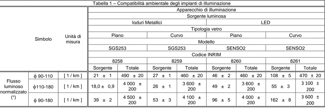
La tabella 1 mostra le valutazioni eseguite estendendo i risultati di misura agli impianti di illuminazione previsti nella fase precedente del progetto di ricerca, adottando le interdistanze di 33 m e 37 m previste rispettivamente per gli apparecchi con vetro piano e vetro curvo.
Come evidenziato nella tabella 1, il flusso luminoso emesso dagli apparecchi di illuminazione al di sopra del piano orizzontale costituisce solo una minima parte del flusso luminoso riflesso dalle superfici illuminate. In percentuale, il flusso emesso direttamente dagli apparecchi non supera il 5% di quello totale. Questa percentuale sale leggermente, non più del 10%, se ci si limita al flusso
Pagina 7 di 25
luminoso emesso e riflesso con elevazioni fino a 20°, ossia la parte del flusso luminoso che più danneggia l’osservazione astronomica: infatti, esso si propaga negli strati più bassi dell’atmosfera, in cui gli aerosol diffondono la luce verso il basso generando la maggior parte della luminanza artificiale del cielo.
Le prescrizioni normative che limitano esclusivamente il flusso luminoso emesso verso l’alto dagli apparecchi di illuminazione non corrispondono quindi in modo adeguato alla situazione fotometrica.
Dalla tabella 1 emerge inoltre che gli impianti con apparecchi con vetro piano sono caratterizzati da maggiori emissioni complessive verso l’alto rispetto agli analoghi che utilizzano apparecchi con vetro curvo. Ne segue che prescrizioni che li privilegiano portano ad una maggiore emissione di luce spuria verso l’alto, contrariamente ai loro obiettivi.
8 Compatibilità energetica
L’analisi riportata in tabella 2 dimostra che gli impianti con apparecchi dotati di vetro piano consumano il 12% circa in più di quelli con apparecchi con vetro curvo.
9 Fattore di luminanza stradale qR (punto 1.2)
Secondo le norme di sicurezza per l’illuminazione stradale, le strade con traffico motorizzato sono illuminate in base a criteri di luminanza media stradale. In Italia, la norma UNI 11248, che deriva dalla CIE 115, prevede 6 categorie
illuminotecniche, da M1 con 2 cd/m2 a M6 con 0,3 cd/m2 per i vari tipi di strada,
luminanze che devono essere rilevate dai conducenti di un autoveicolo con un angolo di osservazione di 1° rispetto al piano stradale.
Per minimizzare il costo energetico e le riflessioni dell’asfalto verso l’alto occorre minimizzare l’illuminamento che genera la luminanza normativa, in quanto sia i consumi energetici sia le riflessioni sono proporzionali all’illuminamento.
Come rilevato dalla pubblicazione CIE 144, è quindi necessario minimizzare il coefficiente QR:
E L
QR
In cui L ed E sono rispettivamente la luminanza e l’illuminamento medio stradale.
Le relazioni tra L ed E dipendono dalle caratteristiche fotometriche del manto stradale, secondo la CIE 144, dalla così detta “tabella r” ed in particolare dal
L’importanza di questo coefficiente, facilmente calcolabile in base ai dati
progettuali, ai fini della valutazione dell’impatto ambientale ed energetico è
confermata dalla pubblicazione CIE 144:
The average road luminance L can be expressed as L = Q E, where Q is an average luminance coefficient of the road surface and E is the average illuminance on the road surface.
When the degree of specular illumination is low (note: typical condition of concrete surfaces), the value of Q0 is close to Qd irrespective of the S1 value.
Accordingly, the uncertainty of the road surface luminance is small.
When the degree of specular illumination if high (note: typical condition of
asphalt surfaces), on the other hand Q approaches and even exceeds Q0. ….
Road lighting with a high degree of specular illumination is typical in most countries because of the resulting gain in average road surface luminance. ….
Pagina 9 di 25
Tabella 1 – Compatibilità ambientale degli impianti di illuminazione
Simbolo Unità di
misura
Apparecchio di illuminazione Sorgente luminosa
Ioduri Metallici LED
Tipologia vetro
Piano Curvo Piano Curvo
Modello
SGS253 SGS253 SENSO2 SENSO2
Codice INRIM
8258 8259 8260 8261
Sorgente Totale Sorgente Totale Sorgente Totale Sorgente Totale
Flusso luminoso normalizzato (°) 90-110 [ 1 / km ] 21 ± 1 490 ± 20 27 ± 1 460 ± 20 46 ± 2 460 ± 20 108 ± 5 470 ± 20 110-180 [ 1 / km ] 18,0 ± 0,9 4 000 ± 200 26 ± 1 3 600 ± 200 49 ± 2 3 600 ± 200 55 ± 3 3 100 ± 200 90-180 [ 1 / km ] 39 ± 2 4 500 ± 200 53 ± 3 4 100 ± 200 96 ± 5 4 000 ± 200 162 ± 8 3 600 ± 200 (°) Flusso luminoso normalizzato rispetto al flusso totale della sorgente in kilolumen per unità di lunghezza dell'impianto
Tabella 2 – Compatibilità energetica
Parametro Condizione Simbolo Unità di misura
Apparecchio di illuminazione Sorgente luminosa
Ioduri Metallici LED
Tipologia vetro
Piano Curvo Piano Curvo
Modello
SGS253 SGS253 SENSO2 SENSO2
Luminanza zona di misura
da corsia di marcia Lmed-,marcia,c [ cd m-2 ] 1,16 1,14 1,40 1,47
corsia di sorpasso Lmed,sorpasso,c [ cd m-2 ] 1,29 1,05 1,52 1,51
Uniformità generale di luminanza
da corsia di marcia Uo,L,marcia [ 1 ] 0,38 0,42 0,45 0,41
da corsia di
sorpasso Uo,L,sorpasso [ 1 ] 0,35 0,47 0,43 0,46
Uniformità longitudinale
da corsia di marcia Ul,L,marcia [ 1 ] 0,56 0,34 0,72 0,71
da corsia di
sorpasso Ul,L,sorpasso [ 1 ] 0,54 0,36 0,80 0,68
Illuminamento Medio Emed [ lx ] 15,03 13,73 15,80 14,77
Coefficiente di luminanza dell'impianto
da corsia di marcia Qi,marcia [ sr-1 ] 0,077 0,083 0,089 0,100
da corsia di sorpasso Qi,sorpasso [ sr -1 ] 0,086 0,076 0,096 0,102 Interdistanza [ m ] 33 37 33 37 Fattore di luminanza qR1 [ sr -1 ] 1,16 1,14 1,32 1,44 1
11
Logo o denominazione del Partner
Nel corso della ricerca è emersa l’opportunità di rendere il coefficiente QR indipendente dal
tipo di asfalto, definendo il fattore di luminanza stradale q0 pari a:
E Q L q 0 0
Il fattore di luminanza stradale è stato inserito nella bozza di revisione della pubblicazione CIE 126 “Guide to the reduction of sky luminance”, allegata alla presente relazione. La CIE 126 prevede il calcolo del flusso luminoso emesso verso l’alto da un generico impianto di illuminazione di una strada con traffico motorizzato, rappresentata schematicamente nella figura 1, mediante la formula:
1) u DLOR ( u ULOR Q q 1 UPF 1 2 R 0 L
In cui UPF è il rapporto fra il flusso luminoso emesso verso l’alto e quello installato, ULOR e DLOR sono i rapporti fra i flussi luminosi emessi rispettivamente verso l’alto e verso il
basso ed il flusso luminoso generato dalle lampade, u il fattore di utilizzazione, ρ1 e ρ2 i
fattori di riflessione della strada e delle zone circostanti e QR il coefficiente medio di luminanza effettivo dell’asfalto.
10 Confronto tra gli impianti (punto 1.1)
La tabella 3 confronta gli impianti oggetto del programma di ricerca dai punti di vista
ambientale ed energetico, utilizzando lo strumento del fattore di luminanza stradale qR.
Alcuni commenti possono essere utili per interpretare la tabella 3.
Il fattore qR è stato valutato partendo sia dai risultati di misura sia (penultima colonna a
destra) da quelli di calcolo (ultima colonna). Mentre i secondi sono coerenti, la dispersione dei primi appare dovuta alle tolleranze di fabbricazione, alle disuniformità dell’asfalto e soprattutto, come messo in evidenza nella relazione dell’INRIM, dalle tolleranze di montaggio sul palo, specialmente per quanto riguarda gli apparecchi a vetro piano.
Il fattore qR dimostra in ogni caso i vantaggi ottenibili dagli apparecchi con vetro curvo
dai punti di vista sia ambientale sia energetico.
Tabella 3 – Riepilogo risultati relativi ad ambiente ed energia Sorg.
luce Vetro
Interdis. [m]
Illumin- [lx] Lumin. [cd/m2] Fatt. lumin. qR
misure calcoli misure calcoli misure calcoli
Ioduri piano 33,00 15 26,0 1,16 1,71 1,10 0,94
curvo 37,00 13,7 20,5 1,14 1,6 1,19 1,11
LED piano 33,00 15,8 16,7 1,4 1,1 1,27 0,94
ACCORDO DI PROGRAMMA MSE-ENEA
Figura 1 Schema di illuminazione stradale
Figura 2 UPF in funzione del fattore di luminanza q0 (a sinistra) e della potenza unitaria
istallata (a destra): gli impianti con apparecchi con vetro piano orizzontale sono rappresentati con simboli aperti crociati, quelli con apparecchi con vetro curvo con simboli pieni. La figura evidenzia che tutti gli apparecchi con vetro curvo presentano migliori prestazioni energetiche e ambientali.
I grafici di figura 2 mostrano la correlazione di qR con energia e ambiente, da cui risulta che elevati valori di questi fattore assicurano minori consumi e minore flusso luminoso
0,8 1,0 1,2 1,4 2 5 10 20 Shallow glass Flat glass Road luminance 1 cd/m2 Lamp power x 1 0 [W/m2 ] Upward flux [lm/m 2 ] U n it a ry u p w a rd fl u x a n d l a m p p o w e r x 1 0
Road luminance factor qR
0,0 0,5 0 5 10 15 Road luminance 1 cd/m2 Shallow glass Flat glass U n ita ry u p w a rd flu x [ lm /m 2]
Unitary installed power [W/m2 ]
13
Logo o denominazione del Partner
emesso verso l’alto, che in base alle misure riportate nelle tabelle 1 e 2 costituiscono la maggior parte del flusso totalmente diretto verso l’alto da parte di un impianto di illuminazione. Si noti in proposito la superiorità degli apparecchi con vetro curvo, tutti con qR>1, mentre con il vetro piano si riscontra qR<1.
11 Città illuminate: sorgenti di luce diffondenti
Quanto detto sopra scoraggia l’impiego di apparecchi di illuminazione con vetro piano installati orizzontalmente, anche perché come dimostrato nella relazione di AIDI del 2010, nella maggior parte delle città gli apparecchi di illuminazione non sono visibili da lontano in quanto nascosti dagli edifici. In conseguenza, le città illuminate si comportano come sorgenti di luce diffondenti e il flusso luminoso emesso verso l’alto dagli apparecchi di illuminazione non ha alcuna importanza: si veda in proposito i grafici della figura 3, tratta
dalla relazione AODI 2010, da cui risulta che neanche il fattore di luminanza qR è più
correlato con la luce verso l’alto di una città diffondente, mentre continua ad essere correlato con l’energia consumata.
Figura 3 Flusso luminoso emesso verso l’alto e consumi energetici relativi ad
apparecchi di illuminazione con emissione nulla verso l’alto, per impianti con apparecchi visibili da lontano (curve blu) e nascosti nelle cavità urbane (curve rosse) per due fattori di utilizzazione.
12 Leggi regionali
Da quanto riferito sopra, appare evidente che le prescrizioni di alcune leggi regionali hanno effetto negativo sulla limitazione della luminanza artificiale del cielo e soprattutto sui consumi energetici, effetto tanto più grave in quanto le prescrizioni di queste leggi valgono su tutto il territorio.
Ciò non significa che non si possa fare nulla per favorire l’osservazione astronomica, ma occorre intervenire intorno ai siti ed in un'area limitata limitando l’illuminazione, evitando di coinvolgere tutto il territorio con prescrizioni che, secondo i risultati di questa ricerca, aumentano i consumi energetici.
0,85 0,90 0,95 1,00 1,05 1,10
0,5 1,0
u=0,4 Luminaires and lit surfac
es visible
bowl cut-off
Luminairea and lit surfaces not visible u=0,5 u=0=0,5 u=0,4 U PF cu t-o ff w io rh l u m in a ire s n d l it su rf a ce s v isi b le
Road luminance factor qR
F1 F2 F3 F4 F5 F6 F7 F8 F9 F10 F11 F12 F13 F14 F15 0,85 0,90 0,95 1,00 1,05 1,10 0,5 1,0 bowl cut-off u=0,5 u=0,4 En e rg y co n su m p ti o s re la ti v e t o cu t-o ff
Road luminance factor qR
F1 F2 F3 F4 F5 F6 F7 F8 F9 F10 F11 F12 F13 F14 F15
ACCORDO DI PROGRAMMA MSE-ENEA
13 Attività futura
Nuove misurazioni e simulazioni per verificare la propagazione sul territorio degli effetti molesti dell’illuminazione stradale, in modo da evitare il ripetersi di prescrizioni estese a tutto il territorio regionale e/o nazionale, con costi aggiuntivi per i cittadini, senza alcun vantaggio per l’astronomia e per l’ambiente e con consumi energetici incrementati.
A questo proposito, INRIM ed AIDI hanno già sviluppato un metodo di analisi che permette di valutare l’influenza delle città illuminate situate intorno ad un sito sulla luminanza artificiale del cielo al di sopra del sito (appendice B).
15
Logo o denominazione del Partner
Appendice A
4 Environmental compatibility
4.1 Artificial sky luminance
The upward emissions and reflections of light generate an artificial luminance of the sky which reduces the contrast of the stars and impairs the astronomic observation. Section 7 reports the relations between sky luminance and limiting magnitude, the quantity which characterises the visual possibilities of an observatory.
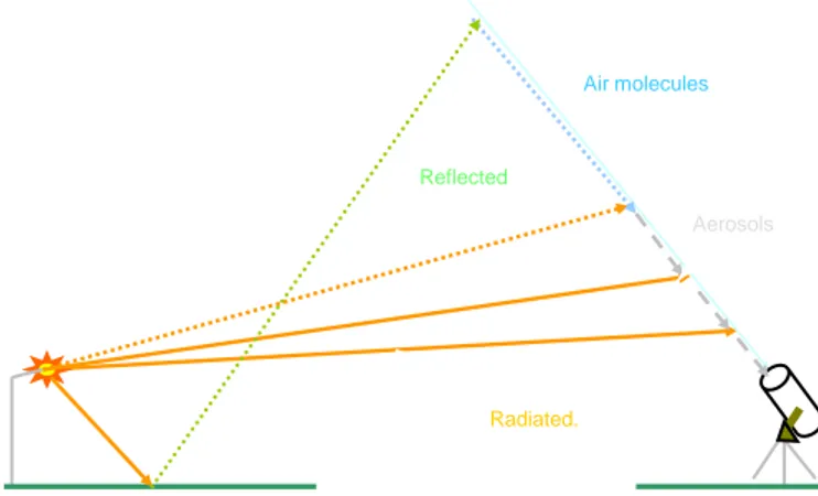
According to the experience of the astronomers, the artificial luminance of the sky is mainly generated by the luminous flux, both emitted directly by the luminaires and reflected by the illuminated surfaces, within the range of elevation between 0° and 20° over the horizontal plane. Actually, at such elevations the light crosses the low levels of the atmosphere, where the veiling luminance generated by the downward diffusion of the aerosol unto the entrance pupil of a telescope reduce the contrast of the heavenly bodies since it adds to the natural sky luminance. The upward light with elevations higher than 20° crosses higher layers of the atmosphere, where aerosol are not present, with a much lower downward diffusion due to the molecules.
Figure 4.1 shows graphically this phenomenon, whose effect on the visibility of the stars is described at section 8.
Direct and reflected rays diagram
Skyglow is caused by the downward scattering of upward light by air molecules and also aerosols, mostly water droplets and dust. The longer the path length through the lowest part of the atmosphere, the more the scattering. Light that goes straight up is mostly reflected, and has shorter paths through the lower scattering layers. The low angle light is mostly directly radiated, and it is this that causes most of the sky glow well away from the source.
Reflected
Radiated.
Air molecules
Aerosols
Figure 4.1 The downward diffusion due to aerosol and molecules in the atmosphere
4.2 Star magnitude
Astronomers evaluate the luminosity of stars according to a scale, established a long time ago through visual assessments of a number of reference stars, whose luminosity was classified in six visually equally spaced levels of “magnitude” (symbol mag), from the brightest to the faintest stars, as visible to the naked eye. This scale was extended when telescopes made much fainter stars visible.
When the background is the natural sky with a very low luminance, the magnitude can be considered equivalent to the luminous flux which enters the entrance pupil of the observation instrument, both the naked eye or a telescope, referred to the same flux due
ACCORDO DI PROGRAMMA MSE-ENEA
to a reference star. Since the area of the entrance pupil is the same for the two stars, it is possible to refer to the illuminances, or to a weighted irradiance, generated by a star on the entrance pupil, be it the of naked eye or of the telescope, in a logarithmic scale2,6. Using lighting quantities (radiant quantities can be used as well):
R R S S M E E log k M (4.1)
k being a scale coefficient, whose usual value is 2,5 mag2, and MR the magnitude of the
reference star R which generates the illuminance ER on the entrance pupil, with the values
of the last two quantities insignificant in this contest. MS increases with lower ES: fainter stars, greater magnitudes. Astronomers measure sky luminance, called brightness, in
magarcsec-2, equivalent in SI units to lx/sr, dimensionally equal to cdm-2.
4.3 Reduction of limiting magnitude due to artificial lighting
With the natural luminance1 LB of the sky in dark places, the naked eye can perceive stars
up to a threshold limiting magnitude MTH ≈ 6 mag, which can be increased through a
telescope to a limit determined on its optical aperture. Over lit areas, upward emissions,
reflections and scatting generate an additional sky luminance LA: the contrast of a large
celestial object like the moon, is reduced and consequently also MTH. Actually, the
detection of an extended object O with a luminance LO against the background luminance
of the sky LB depends on its contrast CO:
B B O O L L L C (4.2)
Luminances are invariant through optical systems: actually, the luminances of the observed object and of its image are equal, except for the optical transmission factors and for the squared ratio of the refraction indices in the object and image spaces, here assumed identical. However, for point sources, like distant stars, the meaning of luminance vanishes and the response of the detecting device (both the eye and a CCD)
depends, as said before, on the luminous flux ϕs through the entrance pupil. The contrast
of a point source is:
B B S S L L h C (4.3)
where h is an appropriate coefficient with the dimension [m-2 sr-1].
Since the sky is never completely black, the magnitude in eqn (1) can be better defined by
the contrast with the natural sky luminance LB 0: this simulates the visual appraisal of the
magnitude of a star with reference to another star of similar known magnitude. From eqn
(4.3), the magnitude MS of a star S can be defined as:
R B R B S R R S S M L h L h log 5 . 2 M C C log 5 . 2 M (4.4)
17
Logo o denominazione del Partner
Suppose that a star with the limiting threshold magnitude MTH of a site is observed with
the natural sky luminance LB. If ϕTH is the luminous flux through the entrance pupil, the contrast is: B B T H T H L L h C (4.5)
Suppose moreover that the same star is observed with some disturbing light sources
around, which generate an additional artificial sky luminance LA. The new contrast CATH
can be obtained adding LA to all luminances in eqn (4.5). From eqn (4.4), since the flux
entering the pupil is the same: B A B T H ATH L L L h C (4.6)
From eqn (4.4), the decrease ∆MTH of the limiting magnitude due to the artificial
luminance LA can be calculated as:
2.5 log
1 a
L L 1 log 5 . 2 C C log 5 . 2 M B A TH ATH TH (4.7)where a=LA/LB. Eqn (4.7) demonstrates rigorously the CIE “sky luminance formula” [1]
4.4 Detection of point-like sources: stars and luminaires
Eqn (4.3) can be written as: B B S S L L E A h C (4.8)
where A is the area of the entrance pupil. Eqn (4.8) recalls that a large entrance pupil of a telescope (i.e., diameter of the lens/mirror) enhances the contrast of a star, while the
influence of the background luminance LB is independent of the entrance pupil: actually,
the telescope behaves like an amplifier of contrasts, as shown by the possibility to observe
bright stars also by day with a high LB.
Eqn (4.8) explains also the preoccupation of the astronomers for the light emitted upward by even small luminaires, which, being point sources, are perceived much better from far away than the luminance of the lit roads, i.e. of extended light surfaces reproduced on the retina as they are. This is probably why many astronomers only ask for cut-off luminaires, without taking care of the consequent increase of the reflections of the lit roads.
It should be noted that a light source can disturb astronomy only if it increases considerably the sky luminance over a site. However, as shown in the following, for far lit towns the sharp attenuation of the spill light with the distance very often does not create any obstacle to astronomy.
ACCORDO DI PROGRAMMA MSE-ENEA
Since a telescope increases the contrast of the stars (see 4.4), an increase in the exposure times there permits to compensate for the effects of the artificial luminance of the sky due to the outdoor lighting installations. However, astronomers do not welcome such procedure since it reduces the potentiality of expensive telescope and reduces the utilization times of an observatory.
19
Logo o denominazione del Partner
Appendice B
7 Environmental compatibility
Frequently, the artificial sky luminance is associated only with the luminous flux emitted upward by the luminaires, with a consequent request to use only luminaires with zero upward emission, generally called “cutoff”, hoping in this way to improve the visibility of the stars. However, the internal reflections of the flat glass for the light at grazing incidence according to the Brewster’s law (figure 6.5) reduce the global efficiency of lighting installations by some 20% [6, 7, 8, 9].
Since about 50% of the luminance of a road is due to the luminous intensities in the range of incidence 60°-750° [10], such types of luminaires are not convenient for energy saving. Moreover, they increase the artificial sky luminance because of the low road luminance
factor qR (see sections 5.2 and 5.3.2), with a higher illuminance necessary for the
luminance levels requested by safety standards [11].
Figure 6.6 A single scheme for all the light components which generate the artificial sky luminance.
Luminaires equipped with distributed light sources, like LEDs, behave in the same way: in all cases the highest efficiencies is with shallow glasses.
Even if the measurements show that the upward luminous flux, which is normally diffused by shallow glasses and not directly emitted by the lamps (see section 6.2 and figure 6.4), is more than compensated by the reduction of the upward reflections of the lit surfaces, it is necessary to verify the relation of such reflections with road luminance, which play a big role also in energy saving programs.
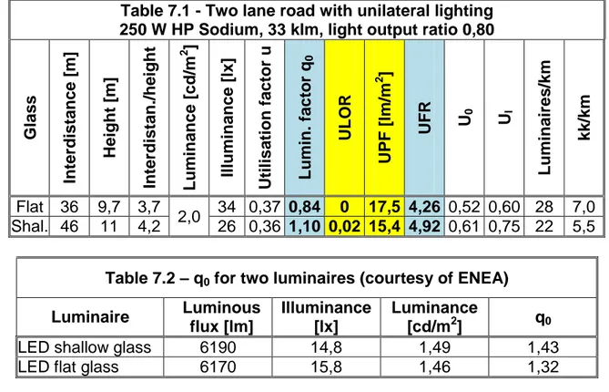
The road luminance factor q0 of section 5.2 plays a major role in lighting design. Table 7.1
shows an example of a calculation on the lighting installation of a two lane road designed according to luminance criteria (class M1 of CIE publication 115), with a luminance of 2
2 0 ° 2 0 ° Diffuse emission from the town
Direct e mission from ins tallation s Diffusio n from the atm ospher e Town 20 ° from insta llations Direct em ission Rural
ACCORDO DI PROGRAMMA MSE-ENEA
cd/m2. The comparison between two types of luminaires, with flat and shallow glass,
shows a large difference for the luminance factor q0, 0,84 and 1,10, respectively for the flat
and the shallow glass luminaires, which leads to a 27% saving in installation costs and energy consumptions for the curved glass, with moreover 31% less in illuminance and thus also in upward light reflections: lower also UPF by 14% for the shallow glass luminaire. Table 7.2 anticipates the results of the test carried out in Italy with the sponsorship of ENEA on some luminaires: again, the shallow glass performs better than the flat glass.
Table 7.1 - Two lane road with unilateral lighting 250 W HP Sodium, 33 klm, light output ratio 0,80
Gl a s s Inter dis tanc e [m] Hei ght [m] Inter dis tan./ he ight Lumina nce [cd/ m 2 ] Il lumi nanc e [lx ] Ut il is a tion f a c to r u Lumin. fac to r q 0 ULOR UPF [lm/ m 2 ] UFR U 0 Ul Lumina ire s /k m k k /k m Flat 36 9,7 3,7 2,0 34 0,37 0,84 0 17,5 4,26 0,52 0,60 28 7,0 Shal. 46 11 4,2 26 0,36 1,10 0,02 15,4 4,92 0,61 0,75 22 5,5
Table 7.2 – q0 for two luminaires (courtesy of ENEA)
Luminaire Luminous flux [lm] Illuminance [lx] Luminance [cd/m2] q0
LED shallow glass 6190 14,8 1,49 1,43
LED flat glass 6170 15,8 1,46 1,32
8 Analysis of the territory
In general, we do not live in a desert. Thus, the choice of a site suitable for astronomic observations or of any restriction to public lighting for improving the visibility of the stars need a preliminary analysis of the lighting territory around the site with the aim of evaluating the possible benefits and the necessary costs.
To start, a correlation should be known a priori with the features of the lighting installations around that site, a difficult task since it depends on unknown atmospheric conditions over the site, the real cause of light pollution.
8.1 Sky luminance formula
It is possible to measure ex post the actual sky luminance LL and also the background sky
luminance LB in a close site with low artificial sky luminance LA and the same atmospheric
pollution, i.e. the minimum sky luminance over a site without any surrounding light source
[6]. The decrease ΔML of the limiting magnitude ML (the highest magnitude of a visible
star) of the site is linked with the artificial and background luminances by the CIE sky glow formula [6]:
21 Logo o denominazione del Partner B L B A B L L L L log 5 , 2 L L 1 log 5 . 2 M M M (8.2) 0.4ML MB B L
10
L
L
where LL = LA + LB is the local sky luminance and MB is the limiting magnitude without
lighting.
8.2 Propagation of sky luminance
The reduction of the nuisances of the external lighting installations is a particular objective of astronomers and ecologists, who report that the light emitted by road lighting at
elevations of 0°-20° (90° γ 110° in the CIE (C,γ) system) produces an artificial sky
luminance also at far distances.
Among there are many models which describe the propagation of the artificial sky
luminance this publication considers the Walker’s law. The artificial sky luminance LA over
a site at a distance D from a light source emitting the luminous flux Φ at 90° γ 110°
(0°-20° over the horizon) can be written as:
LAHD2,5 (8.1)
For dimensional reasons the coefficient H, whose dimensions are m0,5sr-1, was added in
eqn (8.1) to the formula proposed by Walker [12]. Walker’s law is considered valid at an observation angle of 45° in the direction of the source and can be used in this way in the following. However, if the aim is the classification of a site according to all the sources
around it, LA in (8.1) can be at the zenith and supposed to be proportional to the luminance
of Walker’s law.
8.3 Weight of light sources on sky luminance
The basis for any restriction on both urban and rural lighting installations aimed at protecting a site against light pollution should be a cause/effect analysis of the territory
based on the measurement of the local sky luminance LL = LA + LB or of the limiting
magnitude ML at that site and on the influence of each installation h in order to foresee in
quantitative terms both the benefits and the costs as a basis for deciding whether to enforce such restriction or not [25].
An urban installation h is identified with a diffusing source but for a fraction Fh of the luminous flux emitted by the rural installations luminaires visible at low elevations, according to the model described at point 6.5 and in figure 6.6. According to eqn. (8.1), the artificial sky luminance LAh over a site at a distance Dh from that town, with an installed
luminous flux ΦTh, an average reflection factor of the lit surfaces h and an average
ACCORDO DI PROGRAMMA MSE-ENEA
h h h h h
5 , 2 h Th h 20 20 h h h 5 , 2 h Th Ah R F R F 1 e d D K e d R 1 R F F 1 e d D K L (8.1)where e=0,06. The coefficient K depends on local environmental conditions and in the upper line the first and the second terms into square brackets identify urban and rural
sources. Since LA is additive:
h
h 20h
h 20h
5 , 2 h Th n n Ah A L K D d e 1 F R F R L (8.2)where n is the number of the sources h, Fh is the fraction of rural installations, i.e. 1 for all
rural sources and 0 in case of all urban installations. Assuming K constant around a site,
the weight Wh of the source h on LA is:
h 20 h h 20 h h 5 , 2 h Th h h 20 h h 20 h h 5 , 2 h Th B L B Lh A Ah h R F R F 1 e d D R F R F 1 e d D 1 L L 1 L L L L W (8.3)where LLh is the local sky luminance due to the source h.
From eqn (8.3) the relative contribution LAh of light source h to the artificial sky luminance
LA is: 1 L L W 1 L L B L h B Ah (8.4)
ΔML in eqn (8.1) is not a linear function of LA and it is not the sum of all the ΔMLh due to
each single light source h, i.e. ΔML # Σh ΔMLh. However, it is possible to estimate the
effect of the source h on ΔML. The following suggested method evaluates the marginal
reduction δMLh of the limiting magnitude due to the extinction of the source h with all the
other sources operating at their normal level. It follows:
L B h B L h B L Lh L L 1 W 1 log 5 , 2 1 L L W 1 1 log 5 , 2 L L log 5 . 2 M (8.5)δMLh represents the effects of a light source h [25]. Marginal evaluations, frequently used
in economic and financial calculations, are equivalent to a differential at the maximum of a non linear function.
It is to be noted that eqn (8.1) to (8.5) depend on either ΔML or the ratio LL/LB and not on
the actual values of magnitudes and luminances separately. Moreover, all eqn are valid for any type and mixture of sources: urban, rural, parts of towns and even single luminaires.
8.4 Analysis of a site
Often, astronomers and ecologists say that light pollution is additive, at least as far as the artificial sky luminance is concerned. For this reason they propose to reduce to zero any
23
Logo o denominazione del Partner
upward emission in all external lighting installations, this being in their opinion the only way for minimising the artificial sky luminance. However, they do not consider that in this way the unavoidable reflections increase together with the costs for both installation and energy consumption also increase with very little or no benefit for astronomy and for the environment. Only the reduction of lighting levels reduces at the best the sky luminance and, installation costs and the energy consumption [24].
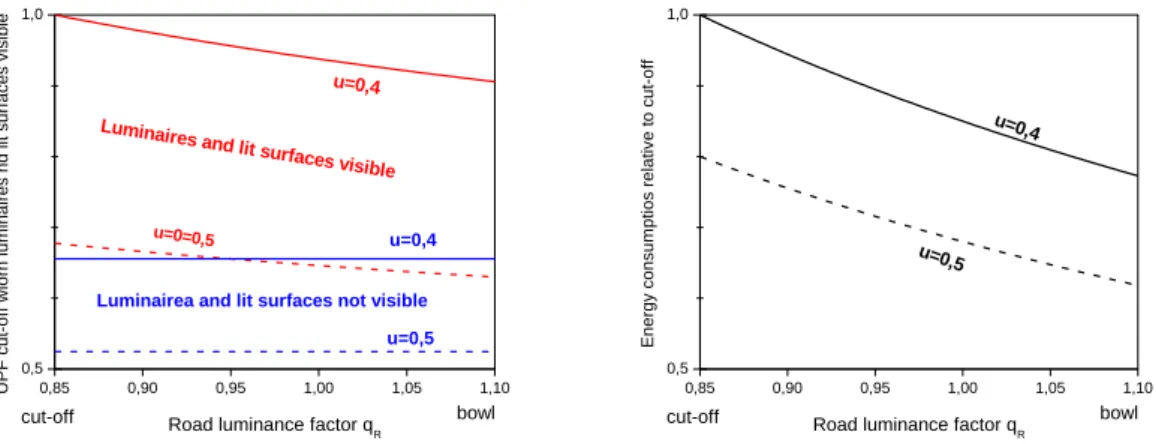
Figure 8.1 Limiting magnitude ML versus LA/LB: the diagrams on the left show no
appreciable improvement through the reduction of R and F, while the functions on the right are the differences between two towns with 100% and 50% road
lighting and show the good increase of ML which can be obtained with a
reduction of 50% of lighting levels [1]
The problem of the reduction of the artificial sky luminance has been based up to now on the additive property of sky luminance through the limitation of the upward direct emissions of the luminaires prescribed in a completely empirical way without any preliminary consideration of the cause/effect relations and on the cost/benefit ratio. However, the additive property does not involve that all light sources contribute in the same way to artificial sky luminance: to cut a little contribution of a source can require very high costs with no appreciable benefit.
Since it is difficult if not impossible to predict the quantitative improvements of the sky luminance and the consequent costs due to empirical reductions of the upward emissions, it is much easier and efficient to change the focal point from the luminaire to the site. The evaluation proposed here of the weight of each light source is an appropriate way for analysing where sustainable costs produce the best benefits in terms of both sky luminance and energy savings. This analysis should be considered a sort of screening of the light sources surrounding a site aimed at verifying which action is more efficient and on which source, preliminary if necessary to more deep analyses. The analysis of the weight of each light source can be carried out through a simple Excel sheet based on the eqn of section 8.3.
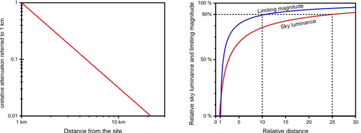
It is not necessary to extend the analysis to very far distances since according to the Walker’s law light attenuation is very quick: figure 8.2 on the left shows the relative influence of the light source versus distance with reference to the same source placed at 1 km from the site and figure 8.2 in the right the relative influence of a uniformly lit territory around a site versus distance on sky luminance and limiting magnitude over the site
0,1 1 10 -3,0 -1,0 -0,1 F = 0 F = 20% R = 10% R = 1% V ariat io n of li m it in g m ag ni tude ML [m ag ] L A /LB F1 F2 F3 F4 F5 F6 F7 F8 F9 F10 F11 F12 F13 F14 F15 F16 F17 F18 F19 0,1 1 10 0,03 0,10 1,00 R = 1 % R = 10% V a ri a ti o n o f l imi ti n g ma g n itu d e M L [ ma g ] LA/LB F1 F2 F3 F4 F5 F6 F7 F8 F9
ACCORDO DI PROGRAMMA MSE-ENEA
starting at 1 km from the site: the decrease of limiting magnitude reaches 90% of its asymptotic value at 10 km from the site.
Figure 8.2 On the left, relative influence of the light source viz distance with reference to the same source placed at 1 km from the site. On the right, relative influence of a uniformly lit territory around a site viz distance on sky luminance and limiting magnitude over the site starting at 1 km from the site: the decrease of limiting magnitude reaches 90% of its asymptotic value at 10 km from the site.
8.5 A case study
An exercise was carried out on an observatory, used today mainly for didactics, placed in Pino Torinese on a hill at 12 km km and about 300 m over the city.
Figure 8.3 is a view of Turin from the observatory. Only about 1000 luminaires are visible out of some 50000 installed in the zones of the town photographed in figure 8.3, demonstrating that Turin actually behaves as a diffusing source.
The analysis included 72 towns within 20 km from Turin, i.e. practically the whole disturbing lit area, since, as shown in figure 8.2, according to the Walker’s law the influence of a light source decreases very quickly with the distance.
Table 8.1 reports the weight in % on sky luminance over the observatory due to 3 towns with a whole weight of 94%. Distance is more important than luminous flux. Pino Torinese with less than 9000 people overcomes Turin with 1 million by 83% to 7%. If necessary, it should be much better to operate on the lighting installations of Pino Torinese: a reduction of 50% of the light levels improves the visibility of the night sky by about 0,6 magnitudes. Of course, this is only a preliminary exercise, which should be completed with local measurements in case of interest.
1 km 10 km 0,01 0,1 1 ù re la ti v e a tt e n u a ti o n re fe rre d t o 1 k m
Dstance from the site
F1 0 1 5 10 15 20 25 30 0 % 50 % 90% 100 % Sky luminan ce Limiting magnitude R el at iv e sk y l umin an ce an d lim it ing m ag ni tud e Relative distance
25
Logo o denominazione del Partner
Figure 8.3 A view of Turin from the observatory. About 1000 luminaires are visible out of some 50000 installed in the part of the town visible, demonstrating that Turin behaves as a diffusion source.
Table 8.1 - Observatory of Pino Torinese - Analysis of territory Contribution to sky luminance of 72 towns around the site
Town Population Distance from
site [km] Contribution to sky lumin. [%] Chieri 33 000 5,8 2 Pino Torinese 8 000 0,7 85 Torino 850 000 12,1 7 68 towns - ≤20 6