On reflection symmetry in natural images

(1)

Alessandro Gnutti

Department of Information Engineering, University of Brescia

Via Branze, 38 Brescia, Italy 25123 a.gnutti006@unibs.it

Fabrizio Guerrini

Via Branze, 38 Brescia, Italy 25123 fabrizio.guerrini@unibs.it

Riccardo Leonardi

Via Branze, 38 Brescia, Italy 25123 riccardo.leonardi@unibs.it

ABSTRACT

Many new symmetry detection algorithms have been recently developed, thanks to an interest revival on computational symmetry for computer graphics and computer vision applica-tions. Notably, in 2013 the IEEE CVPR Conference organized a dedicated workshop and an accompanying symmetry detec-tion competidetec-tion. In this paper we propose an approach for symmetric object detection that is based both on the compu-tation of a symmetry measure for each pixel and on saliency. The symmetry value is obtained as the energy balance of the even-odd decomposition of a patch w.r.t. each possible axis. The candidate symmetry axes are then identified through the localization of peaks along the direction perpendicular to each considered axis orientation. These found candidate axes are finally evaluated through a confidence measure that also allow removing redundant detected symmetries. The obtained results within the framework adopted in the aforementioned competition show significant performance improvement.

CCS CONCEPTS

• Computing methodologies → Image processing; Ob-ject detection;

KEYWORDS

Symmetry detection, even-odd decomposition, saliency map, object detectio.n

ACM Reference format:

Alessandro Gnutti, Fabrizio Guerrini, and Riccardo Leonardi. 2017. On Reflection Symmetry In Natural Images. In Proceedings of CBMI ’17, Florence, Italy, June 19-21, 2017, 7 pages.

https://doi.org/10.1145/3095713.3095743

Permission to make digital or hard copies of all or part of this work for personal or classroom use is granted without fee provided that copies are not made or distributed for profit or commercial advantage and that copies bear this notice and the full citation on the first page. Copyrights for components of this work owned by others than ACM must be honored. Abstracting with credit is permitted. To copy otherwise, or republish, to post on servers or to redistribute to lists, requires prior specific permission and/or a fee. Request permissions from permissions@acm.org.

1 INTRODUCTION

Symmetry is abundant in nature, both at the microscopic (molecules etc.) and macroscopic level (animal and plant species). Many human-made objects also display symmetric elements. As such, symmetry is also present in the digital world as it is an alternative representation of the physical one [5]. So, local and global symmetries play an important part in computer vision and machine intelligence: for example, to simplify object detection [11], to minimize information redundancy [9], to improve source modeling [13] and so on. There is in fact a remarkable interest in this topic, that has led to many symmetry detection algorithms.

The state of the art of symmetry detection techniques up to 2010, surveyed in [9], has most recently focused on bilateral reflection symmetry. The general approach is to recognize symmetries in sets of geometrical objects such as points, line segments or circles [2] or to directly employ the symmetry axis transform (SAT) [3], but such methods are quite sensitive to noise, despite being simple and efficient. More complex approaches have been recently proposed, such as [1], where however it is assumed that the number of symmetry axes is known a priori.

In 2013 the IEEE CVPR conference organized a symmetry detection competition, with two test scenarios: one on a dataset presenting a single main symmetry axis and the other containing multiple symmetry axes. Two works reported the best results, per the survey paper [8]. The first [10] uses constellations of interest points detected using SIFT-like descriptors, and it reports the best results in both test scenarios for recall rates lower than 80%. The second [12], that pairs SIFT descriptors with gradient-based weighting to select symmetry candidates and then validates them with a principled statistical procedure, slightly outperforms the first for high recall ratios. However, in the end, the results were deemed to be not much satisfactory, as argued in [4].

In this paper we propose an algorithm for the detection of symmetric objects in natural images. So, we start with a basic mathematic tool that was proposed in [6] to find hierarchies of symmetries in the raw data for the 1D domain. In that work, detecting whether a 1D digital sequence possesses reflective symmetry is a problem that is solved by decomposing the sequence into its even and odd constitutive parts and then by analyzing their respective energy. The approach is extended here to natural images, i.e. the 2D domain, exploiting spatial correlation properties in the data and using a saliency map to recognize and properly identify the main symmetric object.

(2)

The rest of the paper is organized as follows. We start in Section 2 from a 1D analysis based on the even/odd decompo-sition of discrete sequences. Then, we move to the 2D realm in Section 3 and show how to avoid the pitfalls inherent in the more complex domain. This is shown in Section 4, where we give the details of the symmetry detection algorithm. To properly benchmark it, we used the 2013 CVPR competition dataset. We show in Section 5 that our algorithm outper-forms all of those reported at the end of the competition in [8]. Last, the paper concludes with Section 6.

2 SYMMETRY DETECTION IN 1D

DISCRETE SEQUENCES

We begin presenting a theoretical framework for detecting whether a given 1D discrete sequence possesses reflection symmetry properties to some extent, through the use of the basic even/odd signal basic decomposition. The approach is then extended to the problem of detecting symmetric objects in natural images in the next Section.

Let us consider a real, finite-energy, 1D discrete sequence 𝑥[𝑛], supposing for simplicity sake that it has a finite sup-port. The even/odd decomposition states that 𝑥[𝑛] can be expressed as the sum of an even sequence 𝑥𝑒[𝑛] which is such

that 𝑥𝑒[𝑛] = 𝑥𝑒[−𝑛] and an odd sequence 𝑥𝑜[𝑛] such that

𝑥𝑜[𝑛] = −𝑥𝑜[−𝑛], as follows: 𝑥𝑒[𝑛] = 𝑥[𝑛] + 𝑥[−𝑛] 2 ; 𝑥𝑜[𝑛] = 𝑥[𝑛] − 𝑥[−𝑛] 2 (1)

and 𝑥[𝑛] = 𝑥𝑒[𝑛]+𝑥𝑜[𝑛]. It is readily observable that 𝑥𝑒[𝑛] and

𝑥𝑜[𝑛] are orthogonal in the sense that their inner (or scalar)

product that is defined as < 𝑥𝑒[𝑛], 𝑥𝑜[𝑛] >=∑︀_𝑛𝑥𝑒[𝑛]𝑥*𝑜[𝑛]

is 0. This also implies that the energies of 𝑥𝑒[𝑛] and 𝑥𝑜[𝑛],

respectively 𝐸𝑒 and 𝐸𝑜, sum up to the energy 𝐸 of 𝑥[𝑛].

Of course, this suggests a simple approach to determine how much (anti)-symmetric a sequence is around the time origin 𝑛 = 0. After decomposing the signal 𝑥[𝑛] along the lines of Eq. (1), the more 𝑥[𝑛] is even (resp. odd) the higher (resp. smaller) the energy of the even sequence 𝑥𝑒[𝑛], hence

hinting to a simple approach to determine how much (anti)-symmetric a sequence is: decompose the signal into its even and odd parts and compare their energies. However, this only works if the signal is symmetric around its midpoint.

To approach the problem, it is convenient to generalize the decomposition of Eq. (1) to encompass also the cases when the symmetry is centered around a given point 𝑚. For a real, finite-energy, finite support 1D discrete sequence 𝑥[𝑛], the even-odd decomposition around a point 𝑚 states that 𝑥[𝑛] can be expressed as the sum of an even sequence 𝑥𝑒[𝑛; 𝑚]

and an odd sequence 𝑥𝑜[𝑛; 𝑚] as follows:

𝑥𝑒[𝑛; 𝑚] =

𝑥[𝑛]+𝑥[2𝑚−𝑛]

2 ; 𝑥𝑜[𝑛; 𝑚] =

𝑥[𝑛]−𝑥[2𝑚−𝑛]

2 (2)

and 𝑥[𝑛] = 𝑥𝑒[𝑛; 𝑚] + 𝑥𝑜[𝑛; 𝑚]. Since 𝑥𝑒[𝑛; 𝑚] and 𝑥𝑜[𝑛; 𝑚]

are orthogonal, their energies, that depend on 𝑚 and are referred to as resp. 𝐸𝑒(𝑚) and 𝐸𝑜(𝑚), still sum up to the

energy 𝐸 of 𝑥[𝑛]. When 𝑥[𝑛] is prevalently even around 𝑚

(i.e. reflection symmetric), the energy 𝐸𝑒(𝑚) is more than

half of 𝐸. Therefore, to determine how much symmetric a sequence around a given point 𝑚 is, the signal can be decomposed as in Eq. (2) and 𝐸𝑒(𝑚) is then given by:

𝐸𝑒(𝑚) = ∑︁ 𝑛 |𝑥𝑒[𝑛; 𝑚]|2= ∑︁ 𝑛 ⃒ ⃒ ⃒ ⃒ 𝑥[𝑛] + 𝑥[2𝑚 − 𝑛] 2 ⃒ ⃒ ⃒ ⃒ 2 = =1 4 ∑︁ 𝑛 |𝑥[𝑛]|2+ |𝑥[2𝑚 − 𝑛]|2+ 2𝑥[𝑛]𝑥[2𝑚 − 𝑛] = =1 2𝐸 + 1 2 ∑︁ 𝑛 𝑥[𝑛]𝑥[2𝑚 − 𝑛] = 1 2𝐸 + (𝑥 * 𝑥)[2𝑚] (3)

where in the last passage (𝑥*𝑥) represents the convolution of a discrete sequence with itself (termed in the following as “auto-convolution”).

Local maxima of the auto-convolution correspond to points for which there is good energy decoupling with respect to their immediate neighborhood. Thus, it would appear that local extrema of the auto-convolution can help identify even symmetries. However, take the case where the signal 𝑥[𝑛] has a clear local symmetry but outside the symmetry support the signal is decidedly of higher energy and also possibly non-symmetric. In this case, the samples in the non-symmetric part of the signal leads to a bias in the computation of the energy, to the point of drowning the corresponding auto-convolution value and making the local symmetry no more detectable, as illustrated by Fig. 1. In Fig. 1a an even sym-metry is readily observable (the triangular impulse), but the rest of the signal is just high energy noise with less obvious symmetries. In Fig. 1b the auto-convolution computed on the whole sequence is plotted, and the global maximum is marked with a black circle. It is clear that it is not close to the desired location, namely the center of the triangular impulse, since the non-symmetric surrounding signal has affected the position of the global symmetry point.

The solution to this problem is to limit the convolution support over a basic window centered around the considered point. This way, values of the “windowed” auto-convolution are not affected by the behavior of the sequence in distant po-sitions, which damages the precise detection of the symmetry position when dealing with local symmetries, thus hopefully both compensating for the imprecise location of the true sym-metry point and rejecting false positives in the local maxima due to noise (Fig. 1c). The windowed auto-convolution is then normalized by the energy of the sequence in the window so as to ease the comparison of symmetries between win-dowed sequences having different energy. Alternatively the metric used may become higher just because the signal in the window has higher energy (compare Fig. 1d with Fig. 1c).

To identify the best local symmetry the window is shifted at every location and the normalized auto-convolution is computed for the central point of the window. This in effect corresponds to just computing the inner product between the windowed sequence and its mirrored version, normalizing it by the energy of the windowed sequence. So the measure of symmetry 𝑆 relative to the position in the center of a given

(3)

(a) The original signal, with an artificially created, clear local even symmetry. The symmetry axes as found by the global and local auto-convolutions are also drawn.

(b) The global auto-convolution of the signal shown in Fig. 1a, with the global symmetry marked.

(c) Windowed

auto-convolution of the signal shown in Fig. 1a. A high energy, weaker symmetry can dominate a low energy, stronger one due to the lack of energy normalization.

(d) Windowed, energy nor-malized auto-convolution of the signal of Fig. 1a. Now, the clear even symmetry is dominant.

Figure 1: The effect of windowing and normalization of the auto-convolution to improve the search for local symmetry. The borders where windows go out of bounds are set to 0.

window 𝑊 centered around the considered position, covering 2𝑛𝑝+ 1 positions, is given by:

𝑆(𝑊 ) = ∑︀𝑛𝑝 𝑛=−𝑛𝑝𝑥[𝑛] · 𝑥[−𝑛] ∑︀𝑛𝑝 𝑛=−𝑛𝑝|𝑥[𝑛]| 2 (4)

A last detail to consider is that the best symmetry point may actually correspond to an half-integer position, as the term 2𝑚 in Eq. 3 implies. If we want to retain the same precision in the symmetry detection even after windowing the auto-convolution as in Eq. (4), it follows that the win-dow should be centered at half-integer positions as well. If the computation is confined to the original samples 𝑥[𝑛], it may be a problem to keep the number of positions inside 𝑊 invariant when centered in either integer or half-integer positions. Therefore, 𝑥[𝑛] is interpolated by a factor of 2, doubling 𝑛𝑝and then computing 𝑆(𝑊 ) on the interpolated

image, so that such a computation uses consistent values for adjacent symmetry positions.

3 PRINCIPLES OF SYMMETRY

DETECTION IN NATURAL IMAGES

Our objective is to extend the basic mathematical tool we just derived to solve the problem of symmetric object detection in 2D images. To start, let us consider the case of the search for a vertical symmetry axis, i.e. there is a horizontally symmetric object in the image, clearly perceived by the human eye. To search for symmetry axes in different directions, it may turn convenient to rotate the image first in such a way that the sought symmetry axis becomes vertical.

Using the 1D windowed, normalized auto-convolution pre-viously explained in a row-wise fashion, it should be expected that for all rows passing through the symmetry axis asso-ciated to the object, a local maximum is found exactly in correspondence with a vertical axis. By connecting the re-sulting peaks in the vertical direction the symmetry axis can be simply revealed. However, the noisy nature of data can delete the 1D local symmetry: this possibility is unavoidable, unless much effort is spent in removing the background, com-pensating for illumination changes, or other artefact causes. Our eyes disregard the absence of an actual symmetry in the underlying data for those rows because our brain is able to use the global reflection symmetry information: it extends the symmetric vertical axis and connects it all the way. This suggested us to compute a batch of 1D convolutions all at once for a number of rows, in effect performing the row-wise, windowed and normalized auto-convolution over a 2D square patch. This way, we both correct for noisy placement of symmetry due to image noise and exploit the 2D correlation information present in the image, just like the human brain that would hardly search for 2D symmetry by analyzing separately data along a single dimension.

Consequently a symmetry measure 𝑆2 can be associated

to each center of a 2D patch 𝑃 as follows: 𝑆2(𝑃 ) = ∑︀𝑚𝑝 𝑚=−𝑚𝑝 ∑︀𝑛𝑝 𝑛=−𝑛𝑝𝑥[𝑚, 𝑛] · 𝑥[𝑚, −𝑛] ∑︀𝑛𝑝 𝑚=−𝑛𝑝 ∑︀𝑛𝑝 𝑛=−𝑛𝑝|𝑥[𝑚, 𝑛]| 2 (5)

Each considered possible patch has size (2𝑛𝑝+ 1) × (2𝑛𝑝+ 1).

The averaging taking place by flipping the 2D profile with respect to any considered axis orientation for the whole 2D patch centered at any candidate position is the key of its success. The symmetry axis is correctly extended over adjacent rows independently of the presence of noise and possible slight variations in the object texture.

4 PROPOSED ALGORITHM DETAILS

This Section describes the algorithm proposed for symmetric object detection, including only those details that are deemed essential to properly understand the argument put forward in previous Sections to improve the correct localization and verification of detected symmetry segments.

The objective of the first algorithm part is to compute a symmetry value for all the pixels of the image 𝐼, for any given angle. The values are obtained according to the principles explained in Section 3, and that information is to be stored in a 3D stack. As shown in Fig. 2, such a process is composed of

(4)

Rotation and Interpolation Input Image Map Computation Map Computation Map Computation ˜ Iα1 ˜ Iα2 ˜ Iαn Stacking Mαn Mα2 Mα1 Symmetry Stack

Figure 2: Main processing stages involved in the 3D symmetry stack computation.

three tasks. In the first one, 𝐼 is rotated by 𝑛 different angles 𝛼𝑖to obtain 𝐼𝛼𝑖. The symmetry value is calculated separately

for each angle, so that all possible symmetries can be captured independently of their tilt. 𝐼𝛼𝑖 returns symmetries in the 𝛼𝑖

direction (0 ≤ 𝛼𝑖< 180, with 𝛼𝑖= 180∘𝑖/𝑛; here 𝑛 = 180).

As described in Section 2, the auto-convolution operation applied to a sequence allows to locate the position of the optimal symmetry axis. To improve the location up to half pixel accuracy, a columns interpolation by a factor of 2 is performed on 𝐼𝛼𝑖. So, at the end of the first block of Fig. 2,

𝑛 images are formed, that are referred to as ˜𝐼𝛼𝑖, representing

rotated and interpolated versions of the original image 𝐼. In the map computation process, the level of symmetry of each pixel 𝑝 of ˜𝐼𝛼𝑖 is computed. First, a 2D patch 𝑃 of

fixed size (2𝑛𝑝+ 1) and centered in 𝑝 is extracted. Then, the

symmetry measure 𝑆2(𝑃 ) is computed according to Eq. (5),

that takes values in the [−1, 1] interval. This is strictly related to the ratio between the energy of the signal in the patch and its even-odd decomposition around its middle vertical axis. In particular, 𝑆2(𝑃 ) = 2𝐸𝑒/𝐸 − 1 = 1 − 2𝐸𝑜/𝐸, where

𝐸 is the energy of the signal on the patch and 𝐸𝑒 (resp. 𝐸𝑜)

is the energy of the even (resp. 𝐸𝑜) part of the patch.

The map computation is performed for all images ˜𝐼𝛼𝑖, so

that 𝑛 maps 𝑀𝛼𝑖are generated. Finally, a 3D stack of 𝑛 maps,

in which the 𝑖-th slice is the map 𝑀𝛼𝑖, is constructed. It is

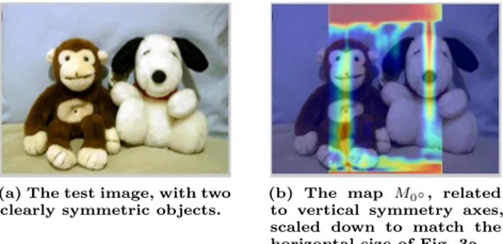
called “symmetry stack” since it represents the local (pixel) information about the level of symmetry. In the example reported in Fig. 3, Fig. 3b shows the computed map for 𝛼 = 0∘ (vertical symmetry axis) superimposed on the test image shown in Fig. 3a. The borders in Fig. 3a are discarded in Fig. 3b since the patches fall outside of the image boundaries. Observe how, in addition to two clear vertical axes where the objects are, the uniform background also exhibits a significant symmetry response.

At this point all symmetry axes present in the image 𝐼 can be identified by processing the symmetry stack. In the end, all candidate symmetry axes are extracted and mapped back to the original image domain. The process is constituted by four distinct operations (see Fig. 4). First, a straightforward (half-wave) rectification is performed, by setting to 0 all negative values of the stack (as done in Fig. 3 too). Following the discussion we have carried so far, one could assume that symmetry measures close to 1 identify stronger symmetries and should be thus sufficient to identify symmetric objects.

(a) The test image, with two clearly symmetric objects.

(b) The map 𝑀0∘, related

to vertical symmetry axes, scaled down to match the horizontal size of Fig. 3a.

Figure 3: The symmetry computation stage for a test image for 𝛼 = 0∘.

On the contrary, we observed experimentally that this is not necessarily true. For example, large values can be associated to uniform background regions that correspond to highly symmetric structures. Moreover, objects that are perceived by humans as clearly symmetric could have lower values due to shadows, illumination changes, low resolution, etc. The use of 2D patches may only alleviate this particular problem.

Instead of just taking the symmetry measure, a key obser-vation is that searching for the peaks (local maxima) of the symmetry map is more relevant. So, the absolute value of the coefficient is not as important as its relationship with respect to its neighbors. All local maxima along the rows of every symmetry map can be associated to a specific direction 𝛼𝑖. A

connectivity analysis between such maxima can be performed by means of a flood-fill algorithm. Consequently, all possible reflection symmetries define a series of segments linking con-nected local maxima existing in each row. Finally, in order to project back the symmetry information onto the original image coordinate system, each map 𝑀𝛼𝑖 is first horizontally

scaled down by a factor 2 to be consistent with the size of the input image 𝐼 and then rotated by −𝛼𝑖.

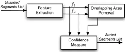
The last part of the algorithm processes the candidate symmetry segments to remove their redundancy, since many segments can be associated to the same symmetry axis but with slightly different slope. In the stack, an axis can be detected in many adjacent slices of the stack, but retaining just one would suffice. In addition, symmetry segments may also be too short, indicating that the symmetry is associated to a small restricted region, or associated to imperceptible symmetries (e.g. background textures). A confidence measure is then attached to the surviving symmetry segments, so that they can be finally sorted in order of importance. Fig. 5 shows the processing blocks involved in this last stage of the algorithm.

We extract a pair of features 𝑓1 and 𝑓2 for each symmetry

segment. The first one is directly connected to the symmetry values that have been computed to detect the considered segment. In particular, 𝑓1 is computed as follows:

𝑓1= ∑︀ 𝑘𝑆2(𝑘) 𝑙 · √ 𝑙 = ∑︀ 𝑘_√𝑆2(𝑘) 𝑙 (6)

(5)

Symmetry Stack

Rectification Local Maxima Search Connectivity Analysis Resizing and Rotation Candidate Symmetry Axes

Figure 4: Main blocks of the candidate axes identifi-cation process, starting from the symmetry stack.

The index 𝑘 in Eq. (6) spans the length 𝑙 of the segment in the slice of the symmetry stack it lays on. In substance, 𝑓1

computes the average value of the symmetry measure 𝑆2(𝑃 )

centered on each point belonging to the segment and then multiplies it by the square root of 𝑙. Experimentally, the normalization by√𝑙 has proven to be a good compromise. It penalizes those segments that are not relevant because they are too short, as mentioned before, while at the same time de-emphasize very long segments since they are likely associated to outstretched background symmetries such as those present in almost uniform regions of the image. The length 𝑙 is actually normalized by the image diagonal size to make 𝑓1

invariant to the image size, so that the symmetry feature can be compared across images with different dimensions.

However, given the particular nature of the competition’s objective, a performance improvement can be expected by another feature added to the symmetry segments process-ing. As a matter of fact, the feature 𝑓1 is more aimed at

the detection of symmetric regions in a given image, and, consequently no particular attention has been placed for fo-cusing on the objects it contains. To reduce the gap between human-perceived symmetry and actual data symmetry, some help is needed by features that can focus on these objects.

A simple approach is employed in this work by computing the saliency map described in [7] to have a quick hint of where objects of interest might be. A second feature 𝑓2 is

computed on the symmetry segments as: 𝑓2= 𝑆𝑀 ·

√

𝑙 (7)

where 𝑆𝑀 is the mean saliency on the locations traversed by the candidate symmetry segment. The product with√𝑙 has the same effect as in Eq. (6). The feature 𝑓2is also normalized

image-wise in the [0, 1] interval by dividing its value by the maximum found for each image.

Finally, the confidence measure for a given symmetry axis is the linear combination 𝛾1𝑓1+ 𝛾2𝑓2 with 𝛾1+ 𝛾2= 1 so as

to give an output still in the [0, 1] interval. The best linear combination can be chosen using a training dataset, as done here to benchmark the algorithm using the framework of the 2013 CVPR competition, or according to the specific require-ments leaning towards either symmetric objects (increasing 𝛾2) or symmetric patterns such as textures (increasing 𝛾1).

Such a feature combination is also used in the redundant segment removal process. The overlapping axes removal block of Fig. 5 is tasked with deleting those segments likely to corre-spond to the same symmetry. To take that decision, the same criterion adopted in the true positives validation step of the 2013 CVPR competition is used. So, two symmetry segments in different slices of the symmetry stack are considered as redundant if the distance between their centers is smaller

Feature Extraction Overlapping Axes Removal Unsorted Segments List f1 Sorted Segments List f2 Confidence Measure

Figure 5: The stages involved in the symmetry seg-ments processing.

than a fifth of the length of the shorter one and in addition the angle that they form is no more than 10∘. To choose the best symmetry segment among a redundant set, of course the one with the best confidence is retained.

The symmetry segments are finally sorted using their con-fidence valus, after the redundant ones are eliminated. An example of the effect of the processing stage described in Fig. 5 is shown in Fig. 6. As it can be seen, the symmetry segments with the highest value shown in Fig. 6b perfectly correspond to the main characters symmetries, while minor symmetries and false alarms in Fig. 6a take on smaller values.

5 EXPERIMENTAL RESULTS

In this Section, the results of the proposed algorithm using the dataset of the 2013 CVPR competition on symmetry detection [8] are reported. The experimental procedure was as follows. The parameters 𝛾1 and 𝛾2 have been obtained

on the training set, maximizing the precision for a recall rate close to 80%. In the experiments the precision was increased by setting a hard threshold 𝑇1for 𝑓1and 𝑇2 for 𝑓2,

since it can be confidently expected that a symmetry axis whose either feature is close to 0 may be safely discarded. The thresholds have been chosen on the training set by maximizing the difference between increase in precision and loss in recall. Fig. 7 depicts the precision/recall obtained on the provided test dataset, for both the single axis and multiple axes detection scenarios. The selected thresholds for both test scenarios are reported too. Such a curve shows very good performance. To put our results in perspective, the precision/recall values obtained from [8] have been drawn on the same graph.

For all conducted experiments, only 4 parameters need to be set: the patch size 𝑛𝑝= 100, the hard thresholds 𝑇𝑖on

𝑓𝑖and the feature weight 𝛾1. The method appeared

exten-sively robust to variations in its parameters. Computational efficiency was not a focus in the current implementation. The average computation time to generate the symmetry stack with a 1∘angular resolution (𝑛 = 180) for an average 213 × 256 image on a standard computer (Intel Core 2 Duo @ 2.13GHz, 4GB RAM) is 220𝑠 using Matlab v2013a. The symmetry stack analysis takes only on average 72𝑠.

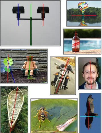
Finally, a collection of visual results is shown in Fig. 8, taken from the provided dataset, that best represent the suc-cess and the limits of the proposed algorithm. The detected symmetry segments, shown superimposed on the images, are

(6)

(a) Unsorted segments list de-tected on the image. Note how some of them traverse symmetric regions that are however not perceived as such by the human eye.

(b) After sorting, the first two segments of the list are indeed associated to the two main perceptual symmetries on the image.

Figure 6: Symmetry segments detection on a test image. Proposed Loy Michaelsen Patraucean Petrosino

(a) Single axis test scenario, using𝑇1= 0.3 and 𝑇2= 0.53. 0.6 0.8 Proposed Loy Michaelsen Patraucean Petrosino

(b) Multiple axes test sce-nario, using 𝑇1 = 0.49 and

𝑇2= 0.53.

Figure 7: Precision/recall curve on the testing set using the the 𝛾1𝑓1 + 𝛾2𝑓2 confidence measure and

hard thresholds as indicated, superimposed to those found in [8].

those obtained with the confidence measure 𝛾1𝑓1+ 𝛾2𝑓2, with

𝛾1 = 0.7, higher than 0.9. Most of them represent

exist-ing symmetries very accurately. Two false positives are also shown in the last row, showcasing two different limits of the algorithm. The algorithm in the ‘eagle’ image is confused by the flat background and by the absence of a truly symmetric content in the supposedly symmetric object. On the other hand, the mis-detection in the ‘bee’ image is caused by the saliency map completely missing the animal and focusing instead on the (though symmetric) bottom right region where the detected symmetry axis is.

6 CONCLUSIONS

In this paper a new method for reflection symmetry axes detection was presented. At its core, a symmetry value is computed using the auto-convolution on a 2D patch for each pixel of the image, suitably rotated for the considered symme-try axis angle and interpolated by a factor of 2, to compute a symmetry map for each angle. These values are extracted by

Figure 8: Collage of visual results on selected images taken from the 2013 CVPR competition dataset.

sliding a window in the horizontal direction and computing the energy-normalized, 2D auto-convolution of the pixels therein. Crucially, candidate symmetry points are chosen not by thresholding the symmetry value but searching for local maxima of the symmetry measure in the orthogonal direction. Once the candidates points are morphologically connected to form candidate axes, they are further processed to remove redundant axes and to assign a confidence value to the surviving ones. The confidence value is a linear combina-tion of the average of symmetry measure itself and the mean saliency, computed along the candidate symmetry segment, added to deal with the specific objectives of the experiments, significantly increasing the precision.

The method has been experimentally validated using the dataset provided during the 2013 CVPR symmetry detection competition. The results outperform all of those reported in [8] for both evaluation scenarios. Such good results are truly remarkable. What is really worth noting is how such a simple fix is enough to achieve good performance. This proves how sound the basic, common-sense considerations that went into the design of the method really are, without any sophisticated use of other features. We plan to make the software freely available for experimentation in the future.

(7)

REFERENCES

[1] I. Atadjanov and S. Lee. 2015. Bilateral symmetry detection based on scale invariant structure feature. In Proc. Int. Conf. on Image Processing (ICIP). IEEE, 3447–3451.

[2] M. Atallah. 1985. On Symmetry Detection. IEEE Trans. on Computers34, 7 (1985), 663–666.

[3] H. Blum and R. Nagel. 1978. Shape description using weighted symmetric axis features. Pattern Recognition 10, 3 (1978), 167– 180.

[4] C. Funk and Y. Liu. 2016. Symmetry recaptcha. In Proc. IEEE Conf. on Computer Vision and Pattern Recognition (CVPR). 5165–5174.

[5] M. Gardner. 2005. The New Ambidextrous Universe: Symmetry and Asymmetry from Mirror Reflections to Superstrings (3 revised ed.). Dover Publications.

[6] A. Gnutti, F. Guerrini, and R. Leonardi. 2015. Representation of Signals by Local Symmetry Decomposition. In Proc. European Signal Processing Conf. (EUSIPCO). 983–987.

[7] J. Harel, C. Koch, and P. Perona. 2007. Graph-based visual saliency. In Advances in Neural Information Processing Systems, Vol. 19. MIT Press, 545–552.

[8] J. Liu, G. Slota, G. Zheng, Z. Wu, M. Park, S. Lee, I. Rauschert, and Y. Liu. 2013. Symmetry Detection from RealWorld Images Competition 2013: Summary and Results. In Proc. IEEE Conf. on Computer Vision and Pattern Recognition (CVPR) Workshops. 200–205.

[9] Y. Liu, H. Hel-Or, C. Kaplan, and L. Gool. 2010. Computational Symmetry in Computer Vision and Computer Graphics. Foun-dations and Trends in Computer Graphics and Vision 5, 1-2 (2010), 1–195.

[10] G. Loy and J. Eklundh. 2006. Detecting Symmetry and Symmetric Constellations of Features.. In Proc. European Conf. on Com-puter Vision (ECCV)(2006-10-30) (Lecture Notes in Computer Science), Ales Leonardis, Horst Bischof, and Axel Pinz (Eds.), Vol. 3952. Springer, 508–521.

[11] N. Mitra, M. Pauly, and D. Wand, M.and Ceylan. 2013. Symme-try in 3d geomeSymme-try: Extraction and applications. In Computer Graphics Forum, Vol. 32. Wiley Online Library, 1–23.

[12] V. Patraucean, R. Grompone von Gioi, and M. Ovsjanikov. 2013. Detection of mirror-symmetric image patches. In Proc. IEEE Conf. on Computer Vision and Pattern Recognition (CVPR) Workshops. 211–216.

[13] V. Sanchez, R. Abugharbieh, and P. Nasiopoulos. 2009. Symmetry-based scalable lossless compression of 3D medical image data. IEEE Trans. on Medical Imaging28, 7 (2009), 1062–1072.