Planning and control of electric distribution networks with integration of wind turbines

Università degli Studi di Salerno

Dipartimento di Ingegneria Elettronica ed Ingegneria Informatica Dottorato di Ricerca in Ingegneria dell’Informazione

XI Ciclo – Nuova Serie

T

D

Planning and Control of

Electric Distribution

Networks with Integration

of Wind Turbines

C

:

G

M

T

:

P

.

P

S

P

.

A

P

C

:

P

.

A

MARCELLI

Acknowledgments

I would like to thank Prof. Pierluigi Siano and Prof. Antonio Piccolo, my advisors at the University of Salerno. Their comments and suggestions throughout the development of this work have been invaluable and are greatly appreciated. I appreciate their time and commitment to my research activities and this work. I also thank them for the opportunity to study and perform research at University of Salerno. I would like to thank Prof. Zhe Chen, for his preciseness and intensive discussions and helpful comments on control of distribution networks when I was visiting scholar at Aalborg University, Denmark.

Dedication

This thesis is dedicated to my father, Esmaeil, my mother, Fatemeh, and my sister, Golpar.

Table of Contents

Chapter 1 Background, Motivation and Contribution ... 1

1.1 Introduction ... 1

1.2 Background and Motivation ... 1

1.3 Literature Review ... 3

1.3.1 Optimal Planning of Distribution Networks with DG ... 4

1.3.1.1 Deterministic Methods ... 4

1.3.1.2 Probabilistic Methods ... 5

1.3.2 Control of Distribution Networks ... 6

1.4 Contributions ... 7

1.5 Thesis Outline ... 8

Chapter 2 Wind Power Challenges ... 10

2.1 Summary ... 10

2.2 A Stimulus for Researchers: Challenges ... 11

2.2.1 A Long Way Ahead ... 12

2.2.2 Wind and Load Correlation ... 12

2.2.3 Generation Mix ... 12

2.2.4 Demand Side Management ... 13

2.2.5 Controllable loads ... 14

2.2.6 Electricity Storage ... 14

2.2.7 Wind Technology Upgrading ... 14

2.2.8 Power System Operation ... 15

2.2.9 Market Design and Clearing tools ... 16

Chapter 3 Planning of Distribution Networks by Using Deterministic Methods ………...18

3.1 The Objectives of DNOs and DG Developers ... 18

3.2 Optimal Placement of WTs by Using Market-based Optimal Power Flow ………...20

3.2.1 The Structure of the Proposed Method ... 20

3.3.1 Constraints ... 22

3.3.1.1 Active and reactive power constraints for the interconnection to the external network (slack bus): ... 22

3.3.1.2 Voltage level constraints at the buses ... 23

3.3.1.3 Thermal limits of the lines connecting the buses ... 23

3.3.2 Dispatchable Load Modeling ... 24

3.3.3 Constrained Cost Variable Formulation ... 25

3.3.4 Step-Controlled Primal Dual Interior Point Method ... 27

3.3.5 Variables ... 28

3.4 Test System Description and Simulation Results ... 28

3.4.1 WTs’ Offers Price Calculation from the Point of View of DNO ... 31

3.4.2 Simulation Results ... 32

3.5 Distribution System Planning within Market Environment ... 35

3.5.1 Aim and Approach ... 35

3.5.2 Modeling of Time-Varying Load Demand and Wind Power Generation ………...36

3.6 GA Implementation for Annual Energy Losses Minimization from the Point of View of DNOs... 39

3.6.1 The Structure of the Proposed Method ... 39

3.6.2 Implementation of GA ... 42

3.7 DNO Acquisition Market ... 43

3.7.1 Simulation Procedure ... 44

3.7.2 Test System Description ... 45

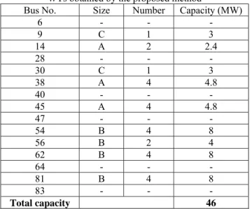
3.7.3 Simulation Results ... 46

3.8 NPV Maximization from the Point of View of WTs’ Developers ... 50

3.8.1 Implementation of PSO Algorithm ... 51

3.8.2 Simulation Procedure ... 54

3.8.3 Simulation Results ... 55

3.9 Discussion and Conclusion ... 62

Chapter 4 Planning of Distribution Networks by Using Probabilistic Methods ………...66

4.1 Modeling Uncertainty ... 67

4.1.2 Wind Turbine Modeling ... 68

4.1.3 Modeling of the Quantity and the Price of WT’s Offer ... 70

4.1.3.1 WT's Offer Quantity Modeling ... 70

4.1.3.2 WT’s Offer Price Calculation and Modeling ... 70

4.2 Structure of The Proposed Method ... 72

4.3 Simulation Procedure ... 74

4.4 Test System Description ... 75

4.5 Simulation Results ... 78

4.6 Discussion and Conclusion ... 84

Chapter 5 Control of Distribution Networks ... 87

5.1 Introduction ... 87

5.2 Grid Code Requirements and FRT Capability ... 89

5.3 Power Electronics for Generators ... 92

5.3.1 Overview of WT topologies ... 93

5.3.1.1 Fixed-Speed WTs ... 93

5.3.1.2 Variable-Speed WTs ... 93

5.3.2 State of the Art Generators ... 94

5.3.2.1 Type A: Fixed Speed ... 96

5.3.2.2 Type A0: Stall Control ... 96

5.3.2.3 Type A1: Pitch Control ... 97

5.3.2.4 Type A2: Active Stall Control... 97

5.3.2.5 Type B: Limited Variable Speed ... 97

5.3.2.6 Type C: variable speed with partial scale frequency converter ... 98

5.3.2.7 Type D: Variable Speed with Full- Scale Frequency Converter ... 98

5.3.3 State of the Art Power Electronics ... 98

5.4 Wind Turbine Generator System ... 99

5.4.1 DFIG-Based WT Capability Limits ... 101

5.4.1.1 Stator Current Limit ... 101

5.4.1.2 Rotor Current Limit ... 101

5.4.1.3 Total Capability Limits ... 102

5.4.1.4 Maximum and Minimum Reactive Power Limits ... 102

5.5.1 Strategy ... 104

5.5.2 Grid Code Requirement and Reactive Power Compensation ... 107

5.6 Description of Fuzzy Logic Controller ... 107

5.6.1 Fuzzification ... 108

5.6.2 Fuzzy Inference Engine ... 109

5.6.3 Defuzzification ... 114

5.7 Case Study and Simulation Results ... 116

5.7.1 Minimum load ... 117

5.7.2 Maximum load ... 124

5.8 Discussion and Conclusion ... 125

Chapter 6 Conclusion and Future Works ... 129

6.1 Summary ... 129

6.2 Conclusions ... 130

6.3 Future Works ... 132

List of Figures

Fig.3.1 The structure of the proposed method ... 22

Fig.3.2 (a) Bid function, (b) total cost function for negative injection ... 26

Fig.3.3 Constrained cost variable ... 27

Fig.3.4 83- bus radial distribution network with candidate locations for WTs ... 30

Fig.3.5 Social welfare ... 35

Fig.3.6 Dispatched active power ... 36

Fig.3.7 Supplied load ... 36

Fig.3.8 Coincident hours for demand/generation scenarios ... 39

Fig.3.9 Schematic example of the coincident hours for two wind profiles (left) and the scenarios (right) ... 40

Fig.3.10 The structure of the proposed method ... 41

Fig.3.11 Schematic of the GA chromosome ... 42

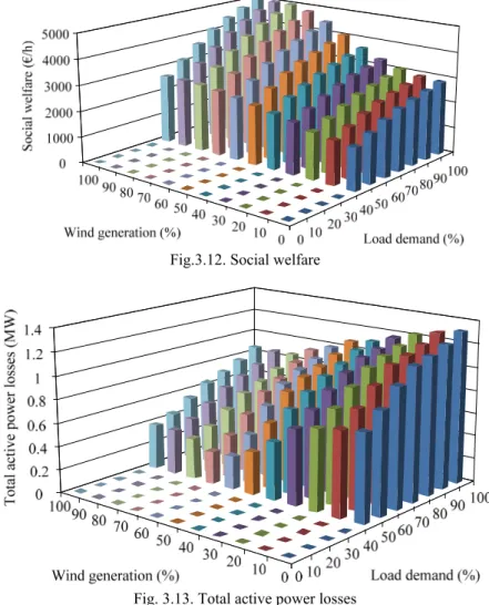
Fig.3.12 Social welfare ... 49

Fig.3.13 Total active power losses ... 49

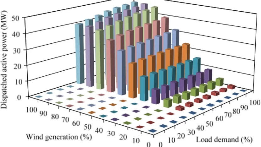
Fig.3.14 Dispatched active power ... 50

Fig.3.15 Percentage of supplied loads ... 51

Fig.3.16 Flowchart of the proposed PSO based algorithm ... 51

Fig.3.17 Dispatched active power by WTs ... 59

Fig.3.18 Delivered energy over the year ... 59

Fig.3.19 Social welfare ... 60

Fig.3.20 Revenue ... 61

Fig.3.21 Supplied loads... 61

Fig.3.22 Total active power losses ... 62

Fig.3.23 Locational marginal price at (a) bus 6 and (b) bus 47 ... 63

Fig.4.1 (a) Typical power curve of a WT, (b) power curve of 660 kW WT ... 70

Fig.4.2 Histogram of a 660 kW WT’s offer price ... 72

Fig.4.3 The structure of the proposed method ... 74

Fig.4.4 (a) Weibull PDF of wind speed, (b) PDF of the WT power output ... 77

Fig.4.5 Mean of injected wind power for different load bands ... 79

Fig.4.6 Mean of LMP for different number of installed WTs and loading levels at (a) bus 14 and (b) bus 54 ... 81

Maximum load ... 83

Fig.4.8 Mean of social welfare for different number of WTs and loading levels 84 Fig.5.1 FRT requirements of the Danish grid code for grids below 100 kV... 92

Fig.5.2 Requirement for reactive power supply during voltage drops ... 92

Fig.5.3 Typical wind turbine configurations ... 95

Fig.5.4 Configuration of DFIG based WT connected to a grid... 100

Fig.5.5 DFIG capability limits ... 102

Fig.5.6 Capability curve of a 9 MW wind farm in normal operation ... 104

Fig.5.7 Schematic diagram of the proposed FRT approach ... 105

Fig.5.8 Strategy of the proposed method ... 106

Fig.5.9 Fuzzy controller ... 108

Fig.5.10 Membership functions of fuzzy controller ... 112

Fig.5.11 Fuzzy surfaces of the controller ... 115

Fig.5.12 25kV weak distribution network... 116

Fig.5.13 (a) wind profile (m/s), (b) generated power (MW) ... 117

Fig.5.14 (a) Voltage at the PCC, (b) reference reactive power at the PCC ... 119

Fig.5.15 Voltage at the PCC ... 122

Fig.5.16 (a) Voltage at the PCC, (b) measured reactive power at the PCC (c) fuzzy controller surface ... 122

Fig.5.17 Active power generated by WFs at the PCC ... 123

Fig.5.18 (a) Voltage and (b) reference reactive power at the PCC during the normal operation ... 124

List of Tables

Table 3.1 Existing wires ... 30

Table 3.2 Loading level ... 30

Table 3.3 Wind generation level ... 31

Table 3.4 Bids of dispatchable loads ... 32

Table 3.5 Financial Data for Estimating WT’s Offer Price ... 33

Table 3.6 Optimal number and capacity of allocated WTs ... 34

Table 3.7 Existing wires ... 46

Table 3.8 Financial data for estimating the offers for a 1.2 MW WT ... 46

Table 3.9 GA parameters ... 47

Table 3.10 The optimal numbers, sizes and capacities of WTs obtained by the proposed method ... 48

Table 3.11 PSO parameters ... 56

Table 3.12 Capital costs of WTs ... 56

Table 3.13 The optimal numbers, sizes and capacities of WTs obtained by the proposed method ... 57

Table 3.14 Results obtained with the proposed method ... 58

Table 3.15 Comparison of the results with GA... 58

Table 4.1 Financial Data for Estimating WT’s Offer Price ... 72

Table 4.2 Loading level ... 76

Table 4.3 Existing wires ... 77

Table 4.4 Bids of Dispatchable loads ... 78

Table 5.1 Wind turbine concept ... 96

Table 5.2 Advantages and disadvantages of using power electronics in WT systems ……….. ... 99

Table 5.3 Rules of fuzzy controller ... 113

Table 5.4 Results obtained with PI controller and without controller for allWF118 Table 5.5 Results Obtained with proposed Controller in the case of 2 WFs ... 120

Table 5.6 Results Obtained with PI and without Controller for All WFs ... 123

Table 5.7 Results Obtained with proposed controller in the case of 2 WFs ... 124  

Chapter 1

Background, Motivation and Contribution

1.1 Introduction

Recently, the wind power penetration into power systems has been increased. The increase in installing wind capacity in the network introduces different challenges to the operation and planning of the network.Nevertheless, wind generation is relied on the wind speed at a specified instant, which is not easy to forecast in advance. The stochastic nature of wind makes its planning a complex problem and therefore there is a need for the existing analytical methods to model the uncertainties related to wind speed properly.

In this chapter, the motivation for the developed methods, a comprehensive literature review and the main contributions of this thesis are described. In addition, the outline of the thesis is provided and the published papers are also listed.

1.2 Background and Motivation

Wind power is one of the most important types of renewable energy sources (RES) for electricity generation in order to reach aims such as the reduction of carbon-dioxide emission, energy autonomy and improved infrastructure reliability.

The intermittent nature of wind introduces some technical and economic challenges that must be overcome in order to integrate wind turbines (WTs) into the electricity networks. Moreover, wind producer has to hedge against the uncertainty and balance the profit variability because of significant wind unpredictability.

The market organization must provide mechanisms to cover energy imbalances caused by wind generation in competitive markets. Wind producers should be able to reduce the costs of imbalances

throughout a market participation that allows them to reinforce their competitiveness.

The impact of uncertainty in wind production can be eliminated by a balancing mechanism in order to compensate the uncertainty of wind power production. Generally, the balancing mechanism is supported by expensive energy sources such as combined cycle gas turbines. Therefore, a main concern of wind producers is that of decreasing the need for energy balancing [1].

Many European countries follow strategies to increase the exploitation of wind energy through incentives and financial alternatives. WTs integration into the grid creates several challenges to distribution network operators (DNOs) such as voltage deviation, power losses and voltage stability [2]. This is mainly due to the mismatch between the WTs place and the potential of local grid to site the new distributed generators (DGs) in the network.

Hence, appropriate placement of DGs in distribution networks has an important role in the improvement of the system operation. The optimal allocation of DGs is one of the most significant aspects for the distribution system planning.

The major role of a DNO is to supply loads at an acceptable voltage and loading level. A DNO has to develop a rational operating strategy taking into account dispatching DGs, interrupting loads, and purchasing power from the wholesale market while keeping system security. In some cases, DNOs play the role of retailers which buy power on the wholesale market at volatile prices and sell it again at fixed tariffs to small consumers. DNOs and retailers are separate market entities with different purposes, networks, and sizes [3].

European Directives 2005/89/EC and 2003/54/EC imply that DNOs should take into consideration the DG placement for planning the expansion of distribution systems. Nevertheless, they do not determine how this will be implemented without coordination between the planners of distribution system and the generation companies. Since the current capacity of distribution system will not be sufficient to deliver the required generated power, different rules have been provided in which a utility is permitted to locate DGs at strategic places on the grid to defer the cost of network upgrade and reduce energy supply costs at peak hours [3].

Supposing that the DNOs aim is to maximize their benefits, two diverse regulatory cases can be taken into account: 1) DG-owning DNO – permitted to possess DG and can exploit the financial benefits considering new generation as a choice for distribution system investments, 2) Unbundled DNO – forbidden to own DG but it can maximize the financial profits considering a number of incentives [4].

The US method for the ownership of DG is driven by the conventional structure of distribution networks in which they are responsible for supplying consumers throughout purchasing power from various sources besides possessing and operating the wires. The financial profits of DG placement to the utility from deferred generation and distribution investments are well recognized and utilities are permitted to place DG at optimal places in the network to defer costs of network upgrade [5].

On the other hand, WTs are typically located in remote and rural areas. In these areas, the feeders are long and operated at a low or medium voltage level characterized by a high R/X ratio and unbalanced voltage situations. Furthermore, weak grids are usually referred to have a 'low short-circuit level' or a ‘low fault level'. In a weak network a change in either active or reactive power can cause a considerable change in the voltage. The impact relies on the strength of the network and the output power of the WTs [6]. Integration of WTs into weak grids will cause the steady state voltage level to go beyond its acceptable limits. Therefore, it can be a constraint for the exploitation of wind energy resources. Another constraint is related to the effect of the power generated by WTs on the voltage quality. Voltage level limitations and accurate control systems are required to control voltage variations as well as to improve voltage quality [7].

In this dissertation, various methods are utilized for planning, management and control of distribution networks with high penetration of WTs.

1.3 Literature Review

Optimal planning methods of distribution networks comprise deterministic and probabilistic methods. In section 1.3.1, previous works that have been carried out to seek the optimal capacities and

locations of DGs with deterministic and probabilistic methods are reviewed. In Section 1.3.2, the methods of control and management of distribution networks during voltage variations are reviewed.

1.3.1 Optimal Planning of Distribution Networks with

DG

1.3.1.1 Deterministic Methods

In [8,9], the authors proposed a genetic algorithm (GA)-based method to determine the optimal sizes and locations of multiple DGs in order to minimize the network losses considering network constraints. In [10], a Tabu search method to obtain the optimal sizes and locations of DGs has been proposed. In [11], the authors proposed a cost based model to allocate DGs in distribution networks in order to minimize DG investment and total operation costs of the network. The objective function is solved using an Ant Colony Optimization method. In [12], a novel method for optimal allocation of DGs in distribution systems to minimize the network losses and to guarantee the acceptable reliability level and voltage profile has been proposed. A particle swarm optimization (PSO) based method for DG placement has been proposed in [13]. The main advantage of this method is that it can be easily implemented and typically the results obtained by this method are converged faster than GA. In [14-16], the use of active management schemes such as the coordinated voltage regulation of on-load tap-changers and the power factor control of DGs, including WTs and diesel generators, integrated in the optimal power flow (OPF) for the optimization of objective function have been investigated. In [17] an optimization technique is suggested to establish the maximum wind power injected into the grid with fixed transmission capacity taking into account the network security. In [18], a numerical algorithm is proposed to estimate the maximum wind energy exploitation in independent electric island networks. In [19], the differences in the improvement patterns of offshore wind power in Europe and US are discussed. In [20] the authors provided an investigation for the wind power investment in Turkey inspiring the

interest of wind investment and evaluating the wind generation costs in this country. In [21], a linear programming model is suggested to specify the optimal technology mix, taking into account wind power production as a negative load that influences the variability of the load profile and therefore the network operation.

1.3.1.2 Probabilistic Methods

In [22], a stochastic formulation of load margin considering power injection uncertainty from RES into the network was proposed. In [23], the authors proposed a single auction market model to evaluate the effect of wind production on market prices and total generation costs for different wind penetration levels and wind farm locations. In [24], a probabilistic reliability criterion considering uncertainties related to component outage in the expansion planning has been proposed. Moreover, the method minimizes the investment budget for constructing new transmission lines considering the uncertainties of the transmission system. In [25], a probabilistic method was proposed to find the wind power capacity limits with regards to the power transfer and voltage constraints in the network. In [26], a stochastic optimization algorithm was proposed to minimize the power losses by controlling the power factor of WTs. Some methods such as point estimation and Fast Fourier transform (FFT) are computationally low-cost while these are less accurate than using Monte Carlo simulation (MCS). In [27], the MCS is used to combine the correlated load demands and wind power generations by using the multivariate distribution to choose random variables. In [28], the authors proposed a hybrid optimization method to minimize the annual power losses to find optimal locations and capacities of WTs. The method combines GA, gradient-based constrained nonlinear optimization algorithm and sequential MCS. The authors in [29] established a well-founded statistical analysis to evaluate the impact of day-ahead wind power forecasts on the performance and the distributional properties of the price in the Western Danish area of the Nord Pool’s Elspot market. In [30], a method for optimal placement of WTs in distribution networks to minimize the annual energy losses has been proposed. The method is based on generating a probabilistic generation-load model that

combines all possible operating circumstances of the WTs and load levels with their probabilities. The problem is formulated as mixed integer non-linear programming to minimize annual energy losses.

Although in [31-34] the impact of wind generations on electricity prices has been investigated, however, there is a lack of mathematical models capable to imitate the amount of the related impact. In [35], the authors provided a review of different computer tools to analyze the integration of renewable sources.

In [36], a hybrid possibilistic–probabilistic tool to assess the impact of DG units on technical performance of distribution network is proposed. The uncertainty of electric loads, DG operation/investments are also considered.

1.3.2 Control of Distribution Networks

In [37], the authors have proposed a mathematical model of the doubly fed induction generator (DFIG) for the analysis of active and reactive power performances of a wind farm (WF). A proportional-integral (PI)-based control algorithm to control the reactive power produced by WTs has been proposed in [38]. In [39], the relation between reactive and active power to maintain the DFIG’s operation within the maximum rotor and stator currents has been studied. In [40], the authors have proposed a fuzzy controller to manage the operation of a Flywheel energy storage system (ESS) connected to a DC bus.

On the other hand, by regulating the rotor blades during abnormal conditions or high wind speed, the active power generated by a WT can be regulated. There are many previous works on pitch angle control. A linear quadratic Gaussian (LQG) control method for controlling the pitch angle has been proposed in [41]. A good robustness in gain and phase margins has been achieved. In [42], the authors proposed a linear matrix inequality (LMI) method for controlling the pitch angle in order to reduce the fluctuations in the power generated by WTs. A robust pitch angle control method has been proposed in [43] for smoothing the variations of the power

generated by WTs. The robustness of system has been obtained by using a LMI method.

Recently, the penetration of WTs into the grids has been increased and the performance of the WTs under faults has become an important issue, especially for DFIGs. Several grid codes prescribed to demand the ability of WTs to stay connected to the grid during faults and voltage variations, referred as fault ride-through (FRT) capability [44]. One of the common FRT capability improvement solutions is to set up a crowbar circuit across the rotor terminals [45]. In [46], the authors have achieved a FRT capability improvement by using hardware modification and inserting an additional voltage source converter connected at the generator terminal. A control strategy for improving the FRT capability by using flexible AC transmission system (FACTS) devices and ESS has been proposed in [47]. In [48], the authors have proposed a new feed-forward transient current control (FFTCC) method applied to rotor side converter for improving the FRT capability. In [49], a fuzzy controller to manage the rotor speed oscillations and the DC-link voltage variations of the DFIG has been proposed.

1.4 Contributions

The main contributions of this thesis are:

1. The review of the main economic and technical challenges of WTs integration into the distribution networks.

2. To provide hybrid deterministic methods for optimal planning of distribution networks with integration of WTs considering wind and load uncertainties. The uncertainties pertaining to wind and load as well as the correlation among different wind speeds are modeled by using time-series analysis.

3. To provide a probabilistic methodology for assessing the amount of wind power that can be injected into the grid as well as the impact of wind power penetration on locational marginal prices (LMPs) throughout the network within market environment considering uncertainties. The uncertainties due to stochastic nature of wind speed and WTs offer price and quantity are modeled by using MCS approach.

4. Policy recommendations for both DNOs and WTs’ developers to better allocate WTs in the network as well as in terms of technical and economic effects.

5. To design a fuzzy controller to improve FRT capability of DFIG based WTs according to Danish grid code. The controller is designed to compensate the voltage variations at the point of common coupling by simultaneously controlling the reactive and active power generated by WTs.

1.5 Thesis Outline

The chapters of the thesis are outlined as follows:

Chapter 2 introduces an overview of the main challenges originated

from the increasing penetration of wind power in distribution systems, and motivates the problems dealt with in this dissertation.

Chapter 3 describes deterministic methods for the planning of

distribution systems within market environment from the points of view of both WTs’ developers and DNOs. The uncertainty in load and wind is modeled by using time series analysis method.

Chapter 4 provides a probabilistic methodology to simulate the

amount of wind power that can be injected into the grid as well as the effect of wind power penetration on LMPs through the network considering uncertainties within market environment. The method is conceived for DNOs to evaluate the amount of wind power that can be injected into the grid.

Chapter 5 describes a fuzzy controller in order to enhance FRT

capability of WTs in distribution networks. The controller is designed to compensate the voltage sages and swells by simultaneously controlling the reactive and active power generated by WTs.

Chapter 2

Wind Power Challenges

2.1

Summary

The climate change issue has sparked discussion on the profits of confining industrial greenhouse gases emissions compared to the costs that modifications would involve. Reaching an agreement on this debatable topic looks to be hard because of the time scales and uncertainties. For the time being, climate change can only be rigorously assessed in relation to the planned effects for the upcoming decades and centuries of swelling temperatures, rising sea levels and heat waves.

Governments in developed countries are at present dependent on public view asking actions to prevent the worst effects of climate change. A major part of these fundamental modifications is to be done in the generation part, where restricting greenhouse gases emissions creates global warming that is currently one of the most important issues. The measures carried out to meet emission reduction goals have principally involved in increasing the penetration level of RES [50-51].

Actually, the US Department of Energy (DOE) defines in [52] a model-based scenario where wind energy caters the 20% of the electricity in the US in 2030, and discusses a group of technical and economic challenges that require to be prevailed for this scenario. The European Union is presently following the execution of its ambitious 20/20/20 goals, which aim by 2020 to decrease greenhouse gas emissions by 20%, compared to 1990; increase the amount of RES to 20% of the supply of energy, and the energy consumption decrement by 20% by means of energy efficiency schemes [53]. Numerous European countries, for instance, Germany, Spain, Portugal, and Denmark, have already achieved high wind power integration into the network in the range of 7 to 20% of electricity consumption. The rapid

growing of installed capacity of wind power is predicted to carry on in Europe and the United States [54-56]. It is expected that Asia will become the area in the world with the greatest development of installed wind capacity in the near future. This development will be mostly obtained by China, which has been increasing its installed capacity each year for the preceding few years, and is set to carry on the fast increment of its wind capacity to become the world’s biggest annual market. Actually, annual augmentations are anticipated to reach more than 20 GW in China by 2014 [57]. This great advance is vigorously stimulated by government strategies intended to promote the supply change, inspire the development of the domestic industry, and undertake the network planning and strengthening needed to acquire the electricity to the market.

2.2 A Stimulus for Researchers: Challenges

Wind power has no emissions and assists sustainable growth. The wind generation is renewable source and geopolitically generous, encouraging the self-reliance in energy of states. Furthermore, it doesn’t use water. As WTs do not use fuel, costs can be reduced and they can be a barrier against the volatility of fuel price. Note that wind power plants have low enforced interruption rates and can help to diminish the requirement for contaminating generation sources.

Nevertheless, because of the uncertainty of wind power it can’t be dispatched in a conventional sense. Accordingly, as wind power is variable and uncertain, the high penetration of wind power into a network creates challenges for network operators and planners in about all the fields of the electrical power systems [58-61].

In fact, the handling of uncertainties in a network isn’t new for specialists. Note that loads are also stochastic and variable and the network operators have been tackling the variability and uncertainty of loads.

2.2.1

A Long Way Ahead

The wind power integration into a grid requires taking into account a greater amount of uncertainty and variability in the grid operation. This fundamental fact becomes of the most importance if considering the crucial wind power integration into the grid denotes that numerous countries all over the world have set out to reach.

The wind power production variability entails the power system operation with a greater flexibility degree to coordinate the load variation that is described as the difference between the total energy consumption and the total wind energy production. This flexibility characterizes the grid capability to integrate wind power. The requisite for improving the flexibility to embed the variability of wind is depending on a number of features of a power system as explained in the following.

2.2.2 Wind and Load Correlation

If the daily pattern of wind power production coincides with that of demand, wind variability can be absorbed by consumers, with the subsequent decrease in net load variations.

Generally, load and wind availability are not correlated, for example, in Northern Europe, albeit the historical archives disclose that wind power production in winter is greater than that in the summer, there is not a notable coincidence of winter periods with high load and high wind generation [62]. Correlation between wind speeds at two diverse places typically decreases with their distance [63]. Furthermore, the variations of wind farms output power, fed with uncorrelated winds, are neutralized and consequently, the variability of total wind generation reduces. Hence, the geographical distribution of wind farms has a smoothing impact on wind power fluctuations. However, decisions on the location of WTs are usually limited to the wind availability that can be beneficially used.

2.2.3 Generation Mix

Indeed, the capability of a power system to integrate wind power is toughly reliant on its generation mix. Production technologies

capable to proficiently change their power output as needed by the net load fluctuations are of required to withstand supply paradigm mainly based on renewable energy sources. Actually, generally when there is unfavorable correlation between wind and load, not only the necessity for cycling units is increased considerably but also the operating system of the units will be changed considerably. In this regard, flexibility on the generation-side of a power system generally results in operating conventional units at levels of productions greater or less than their optimal to accommodate the intrinsic variability of wind generation by ramping up or down. Moreover, the ramping expeditions may mostly end up with the start-up or shut-down of conventional generators. Accordingly, if great fluctuations of wind generation are to be accommodated by the conventional generation, this may lead to conventional power plants work in a less proficient way, therefore decreasing the amount of pollutant emissions that are decreased by the wind energy integration into the grid [64]. The pollution reduction reached by wind integration is reliant on the type of production and fuel that is substituted when WTs are generating.

Note that wind power integration has an important effect on the generation mix of a power system. The appropriate assessment of this impact needs calculating the wind generation’s capacity credit [65].

The capacity credit is a criterion to measure of the volume of conventional generation that is substituted by the intermittent generation without decreasing the reliability of the system. However, when the reliability of the power plant is less than 100%, there always exists a confined risk of not having sufficient capacity accessible to satisfy the demand, and wind generation may be accessible at the crucial moment when load is high and other generators may fail. Actually, it implies that 1 MW of installed wind capacity is not enough to cover 1MWof demand in a reliable and safe way, but it is sufficient to effectively satisfy a specified percentage of it [66].

2.2.4 Demand Side Management

If wind generation and demand are not correlated and the weather conditions cannot be changed, a technique is introducing demand response method to utilize the real-time pricing (RTP) [67-70], according to which retail prices alter mostly to reflect fluctuations in

the energy dispatch and the cost of supplied load. If wind is high/low, the demand will increase/decrease because of low/high prices while when wind is low the demand will decrease due to high prices. The accomplishment of demand-side management schemes will be significantly facilitated by the constitution of smart grids [71], which are considered to enable consumers to play a significant role in optimization of power systems operation by means of intelligent monitoring, control, and communication.

2.2.5 Controllable loads

The controllable loads could be added to the grid to use the unused wind power production. For instance, some kinds of these loads comprise electric heating, and boilers, fuel production such as hydrogen heating; and the electric vehicles or plug-in hybrid vehicles (PHV) that is becoming a hopeful potential in large-scale applications [72,73]. The implication of vehicle-to-grid (V2G) refers to a system where PHVs connect to the network to cater services of demand response by injecting/absorbing power into/from the grid [74, 75].

2.2.6 Electricity Storage

The technical community decides that the high penetration of RES can be significantly simplified by increasing significant storage capabilities. Albeit currently there are numerous energy storage technologies that can afford to achieve this goal such batteries, flywheels, electric vehicles, superconducting magnetic energy storage systems, compressed air, pumped hydro storage systems [76, 77]. Innovative developments and more incentives in this arena are still required for the huge electricity storage to become a reality in the requisite terms [77, 78].

2.2.7 Wind Technology Upgrading

A part of electricity supply side requires to be supplied by generators to cater the ancillary services needed to guarantee the safe operation of the power system. If WTs are not equipped with the proper technology to help the voltage control devices, wind curtailments will be unavoidable in conditions where the sum of the

wind generation and the conventional generation is essential for safety reasons exceed energy consumption. In some countries, grid companies are forcing generators to set up tools for voltage and reactive power control [65]. Furthermore, the significant amount of wind power penetration into the grid requires that WTs stay connected to the grid during fault.

2.2.8 Power System Operation

As previously stated, wind power encompasses uncertainty and variability in the power system operation. A part of the uncertainty can be expected several hours or days ago and can be absorbed by an optimal energy dispatch of the network operators according to their elasticity. Essentially, a generator or load that caters reserve want to change its generation as needed in a short time. Reserves needed to incorporate unexpected wind power variations are basically slow, i.e., the activation times are about or more than 15 minutes [60].

The extension of reserves results in comparatively fast energy re-dispatches, which considerably augments the need for elasticity of power system elements. Accordingly, wind uncertainty includes also operating costs [60, 61] that can be minimized by proper reserve placement and deployment. Briefly, tools for the optimal energy and reserve scheduling are critical to optimal use of wind power in order to avoid unnecessary wind power curtailments and reducing the costs of expected or unexpected uncertainty.

In most countries, the wind energy development is happening in a reconstructed electricity area are controlled by market rules. Electricity transactions are therefore complied in a market to which generators and loads submit their bids to maximize their benefits or minimize the procurement costs. A third party, generally referred to as market operator (MO), is responsible to determine the accepted bids of producers and consumers as well as the electricity price. The aim of MO is maximizing SW by using a market-clearing tool. The competitive transaction of the electricity is challenging by itself because of the constraints forced by the grids and their agents, and they will be influenced by uncertainties. The aim of the market is augmenting the financial performance of grids while ensuring a safe action of the electrical structure.

2.2.9 Market Design and Clearing tools

Every electricity market is established adversely. Usually, electricity markets comprise numerous trading areas to assist energy transactions between producers and consumers in the long and short run. Trading levels for short-term energy trading encompass a day-ahead market, numerous adjustment and balancing markets.

The set of these serially organized short-term trading levels is typically referred to as the pool. In the day-ahead market, energy trading to be happened in the following day is discussed. The adjustment markets allow market operators to change the energy sold or purchased in the day-ahead market with regards to modifications in their expected generations or consumptions. The balancing markets, so-called real-time markets, enable last minute energy trading to tackle with real situations and assure the actual balance between generation and load. The Electricity Market of the Iberian Peninsula, for example, comprises one day-ahead market, six adjustment markets consecutively organized over the delivery horizon, and hourly balancing markets [79].

The results of an electricity market are depending on the market clearing procedure utilized by the market operator. Presently, there are different market-clearing methods such as single auction methods and complex mechanisms for the concurrent energy provision and reserve by means of an OPF. Generally, the market-clearing device’s complication depends on the properties of the network that are taken into account in the procedure. Therefore, the techniques for market clearing may consider inter-temporal constraints such as the ramping capabilities or the minimum up and down times of generators. The tool for pricing is dependent on the market clearing mechanism. Therefore, the network modeling in the process to clear the market results in the concept of LMP in which, the LMP at each bus of the network is diverse because of active power losses or network congestion [76,80,81]. On the contrary, if the constraints of the network are neglected, a unique price is attained.

Chapter 3

Planning of Distribution Networks by Using

Deterministic Methods

This chapter introduces deterministic methods for optimal planning of distribution networks within a distribution market with integration of wind turbines. Section 3.1 introduces the objectives of DNOs and DG developers. Section 3.2 introduces an innovative method for optimal placement of WTs in distribution network by using OPF. Model formulation is explained in Section 3.3. Test system description and simulation results of this method are provided in Section 3.4. In Section 3.6, the GA implementation for annual energy losses minimization from the DNOs viewpoint is explained. DNO acquisition market is introduced in Section 3.7. Section 3.8 discusses the net present value (NPV) maximization from the point of view of wind turbines’ developers. The discussion and conclusions are provided in Section 3.9.

3.1 The Objectives of DNOs and DG

Developers

This section investigates the DNOs and developers incentives, which they are two main actors in DG market. The objectives of DG developers are maximizing returns from electricity sales and minimizing the imported energy cost when there are combined heat and power (CHP). These will tend to be met with augmented installed capacity but they are considerably affected by the strategies of DNO on connection and use of system charges.

The incentives for installing DG are different. Some countries such as Australia and Ireland use deep charging while some others like Italy, France and Norway apply shallower charges [82, 83]. In the United States, customers are responsible for paying costs beyond a regulator-specified connection “allowance” [82]. Most systems do not

presently apply Distribution Use of System (DUoS) charges to DG except in a few cases such as Sweden and the U.K., DG placement in the distribution systems of U.K, before April 2005, was charged the full capital costs of connection, and capitalized operation and maintenance costs instead of DUoS charges [84].

The charges encourage the DNO to site DG by catering a return more than the normal regulated return rate in which there is a rational take up level and use of connected generation and the costs of connection are comparatively low [83]. Finally, the cost of network connection and usage is driven by the match between the DG capacity and the network to which it connects. According to the U.K. incentives for DNOs, there is profit to DNOs and DG developers in reducing the capital costs related to reinforcement. Although active network management schemes [85] make a major contribution, identifying and encouraging DG connections at sites and capacities that make the best use of the network is required [86-89].

However, 7% of electricity produced in the U.K. is lost as power losses. Although losses are unavoidable, they can be controlled via investment in low loss tools and more efficient network configuration [90]. Moreover, losses can be considerably affected by DGs: power injections at low voltages reduce losses but losses may increase generally when the injected power is higher than demand. Though the DG effect on losses is site and time specific, losses track a U-shaped trajectory [91]. Till 2005, the DNO incentives to reduce losses were by loss adjustment factors (LAFs) [92] with site-specific LAFs applied at 33 kV and above. The price control motivates DNOs to control losses through catering rewards for loss reductions and penalties for increases compared with a target level. The annual target of DNO is set by Office of Gas and Electricity Market (Ofgem) and values losses at 60 €/MWh (according to 2004 values). DNOs are encouraged to be responsible the essential investment to reduce the losses [83]. The low amount of DG penetration to reduce the power losses can motivate DNOs to confine connections within their networks. It should be noted that DG developers are not fully incentivized for their impact on losses.

3.2

Optimal Placement of WTs by Using

Market-based Optimal Power Flow

In this section, a novel method for optimal allocation of WTs by using market-based OPF to maximize the system SW is proposed. The market-based OPF uses constrained cost variable (CCV) approach to generate the appropriate helper variable, cost term, and related constraints for any piecewise linear costs. The method is conceived for DG-owning DNOs to find the optimal numbers and sizes of WTs among different potential combinations. WTs and dispatchable loads (DLs) are owned or managed by the DG-owning DNO. The objective function is solved by using step-controlled primal dual interior point method (SCPDIPM) considering network constraints.

The proposed method considers SW maximization for the optimal allocation of WTs, thus, its maximization implies not only the minimization of the energy production costs but also the maximization of the consumers’ benefit.

By using the proposed method, WTs can be, in fact, optimally allocated at buses where they are more advantageous, i.e. near higher loads or in parts of the network where the loads have the higher values and the consumers’ benefit is higher. The method can help DG-owning DNOs to better allocate WTs by considering cost reduction and consumers’ benefits.

3.2.1

The Structure of the Proposed Method

The structure of the proposed method for optimal allocation of WTs is shown in Fig.3.1. The method maximizes the SW by using market-based OPF for different combinations of load demand and wind power generation considering network constraints.

Different combinations of wind power generation and load demand is considered via scenarios. Each demand level is characterized by six wind generation levels. There are four load demand levels, i.e. 30%, 50%, 70%, 90%, and six wind generation levels, i.e. 0%, 20%, 40%, 60%, 80%, and 100%. Therefore, jointly considering the load demand and wind generation levels results in 24

scenarios, i.e. four load demand levels, with two blocks per level with different sizes and the same price, by six wind generation levels with four blocks per level with the same size and the same price for all blocks.

The maximum number of WTs that can be allocated at a given bus is represented by an equivalent number of blocks in the WT’s offer. At each candidate bus it is assumed that maximum four WTs can be allocated; therefore, for each generation level there are four blocks with the same price and the same size equal to the rated power of the WTs for all blocks. With regards to the bids for DLs, it is assumed that there are two blocks per load with different sizes and the same price for all blocks, respectively.

The market-based OPF uses CCV method to generate the appropriate helper variable, cost term, and related constraints for any piecewise linear costs. WTs’ offers and bids of DLs are taken and treated as marginal cost and marginal benefit functions, respectively, then by using the CCV method they are converted to the equivalent total cost and total benefit functions and plugged into a matrix as piecewise linear costs. The method is applied by DNOs to find the optimal numbers and capacities of WTs among different potential combinations.

Fig.3.1.The structure of the proposed method

3.3

Model Formulation

In this section, the mathematical formulation of SW maximization is discussed. Maximization of SW implies not only the minimization

of the energy production costs but also the maximization of the consumers’ benefit. The SW is formulated as follows:

Maximize 





b

m

g

p





b is the intercept (reservation price bi> 0) in €/MWh, g

m is the slope (mg> 0) in €/MW

2_h,

i

p is the price at which producer i is willing to supply in €/MWh, i g is the supply in MW, j d j j b m d p   , for j1,2,_J (3.5) where j

b is the intercept (reservation price b > 0) in €/MWh, _j d

m is the slope (m < 0)in €/MWd

2_h,

j

p is the price at which consumer j is willing to pay in €/MWh, j

d is the demand in MW.

3.3.1

Constraints

3.3.1.1 Active and reactive power constraints for the interconnection to the external network (slack bus):

max min b b b P P P   , min max b b b Q Q Q   (3.6)

where P and _b Q are active and reactive power of the slack bus, _b

respectively.

3.3.1.2 Voltage level constraints at the buses max min i i i V V V   (3.7) where min i V and max i

V are the lower and upper bounds of the bus voltage, respectively.

3.3.1.3 Thermal limits of the lines connecting the buses The thermal capacity max

k

S of network also bounds the maximum

apparent power transfer,Sk:

0 max _ S_k S (3.8) 3.3.1.4 WTs power constraint max 0P_g P_g (3.9) It is assumed that WTs operate at constant power factor.

2 2 cos g g g Q P P    =constant. (3.10) where Pgand Qgare the generated active and reactive powers by WTs,

respectively. 3.3.1.5 DLs power constraints 0 min _{ } d d P P (3.11)

It is assumed that DLs operate at constant power factor.

2 2 cos d d d Q P P    =constant. (3.12)

3.3.2

Dispatchable Load Modeling

One way to model price-sensitive or DLs is modeling them as negative generators with related negative costs. This is carried out by determining a generator with a negative output in a range from a minimum injection equivalent to the negative of the highest load value to a maximum injection of zero [93,94]. Here, it is supposed that DLs have a fixed power factor and an equality constraint to impose a fixed power factor for a negative generator is utilized for a DL modeling. It should be noted that with the description of a DL as a negative generator, if the negative cost relates to the consumer’s benefit function, the minimization of generation cost is equal to SW maximization.

Furthermore, an additional equality constraint to enforce a constant power factor for any “negative generator” is utilized to model a DL. In the following, an example of a DL is provided whose marginal benefit function is shown in Fig. 3.2 (a). This relates to a negative generator with the piecewise linear cost curve as shown in Fig.3.2 (b). It should be noted that this approach assumes that the demand blocks can be partially dispatched or split.

(b)

Fig.3.2. (a) Bid function, (b) total cost function for negative injection

3.3.3

Constrained Cost Variable Formulation

The conventional OPF formulation is not capable to solve the non-smooth piecewise linear cost functions result from discrete offers and bids, thus, when such cost functions are convex they can be modeled by CCV method [95-97].

The market-based OPF uses CCV method to generate the appropriate helper variable, cost term, and related constraints for any piecewise linear costs. CCV is an alternative OPF formulation that is suggested to enhance the market-based OPF scalability computation. The piecewise linear cost function c(x) is replaced with a helper variable y and linear constraints that produce a convex “basin” needs the cost variable y to put into the functionc(x). A convex n-segment piecewise linear cost function is shown in Fig. 3.3.

Fig.3.3. Constrained cost variable                    x x c x x m x x x c x x m x x c x x m x c n n n n 1 2 1 2 2 2 1 1 1 1 , ) ( , ) ( , ) ( ) (  (3.13)

A convex n-segment piecewise linear cost function is defined by a sequence of points(x_j,c_j), j0_n where m denotes the slope of _j

the jth segment, 1 1      j j j j j _{x x} c c m , j_{1 }, ,n (3.14) and x0 <x1 < ··· <xn and m1 ≤ m2 ≤··· <mn.

The “basin” related to the cost function is generated through the following n constraints on the helper variable y.

j j

j x x c

m

The variable y is added to the objective function instead ofc(x). By using CCV method, the piecewise linear costs of active or reactive power can be converted into the appropriate helper variable and the related constraints.

Furthermore, every piecewise function in the objective is substituted with a helper variable and for every piece of the piecewise function inequality constraints are imposed on that variable. CCV is a way that formulates a piecewise linear cost function on a new variable that is linearly constrained.

In this thesis, the offers of WTs and bids of DLs are taken and treated as marginal cost and marginal benefit functions, respectively, then by using CCV method they are converted into the equivalent total cost and total benefit functions by integrating the marginal cost and benefit functions and plugged into a matrix as piecewise linear costs.

3.3.4

Step-Controlled Primal Dual Interior Point

Method

The Primal Dual Interior Point method (PDIPM) and its numerous variations have become the algorithms of choice for solving OPFs in the last years [95-97].

Even if the PDIPM fits properly with classical OPFs that utilize smooth polynomial cost function, it is not able to solve the market-based OPFs with non-differentiable piecewise cost. When piecewise cost is considered, the gradient and Hessian variables change from iteration to iteration considerably. Also, the descending of Newton steps is not obtained. The SCPDIPM [93, 94] that is used in this paper overcomes this difficulty by monitoring the accuracy of the quadratic approximation of the Lagrangian during the OPF computation and reducing the Newton step if any unexpected change of derivative results in an inaccurate approximation. It is efficient applying such step control method when the normal PDIPM step is not able to improve the gradient condition. By adjusting steps, SCPDIPM is able to reduce both system cost and gradients.

3.3.5

Variables

For the objective function (3.1) the optimization variable including vector L= [V_i,_i,P_g ,P_d ] where V_iand _iare voltage and voltage angle at the buses, respectively.P is active power generated by WTs g

and Pdis active power of DLs.

and are Langrangian multipliers and uses the Newton’s method to solve the Karush–Kuhn–Tucker (KKT) conditions [93-95].

3.4 Test System Description and Simulation

Results

In this section, the distribution system used to test the proposed method is described. The following analyses are based on an 83-bus 11.4-kV radial distribution system whose data given in [4]. The eleven feeders are supplied by two 20 MVA, 33/11.4 kV transformers. The one line diagram of the distribution system is shown in Fig.3.4. The candidate buses in the test system are included in the set {6, 9, 14, 28, 30, 38, 40, 45, 47, 54, 56, 62, 64, 81, 83}. The WTs operate at power factor of 0.95 lagging. Voltage limits are taken to be ±6% of nominal value, i.e. Vmax= 1.06 p.u. and Vmin= 0.94 p.u., and the feeders’

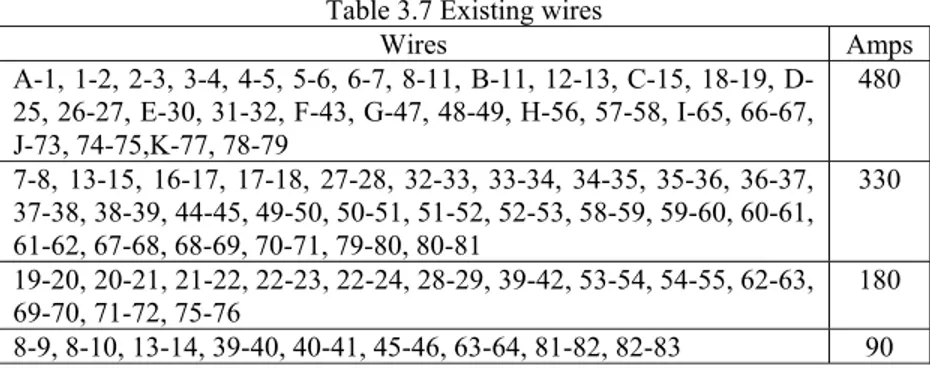
thermal limits are given in Table 3.1 and vary between 40 and 480 A. Dispatchable and fixed loads, with constant power factor equal to 0.95, are served by both the grid and the WTs. The total maximum fixed load is 5.4 MW. The loading level for each band is given in Table 3.2.

Fig.3.4. 83- bus radial distribution network with candidate locations for WTs Table 3.1 Existing wires

Wires Amps A-1, 1-2, 2-3, 3-4, 4-5, 5-6, B-11, 12-13, C-15, D-25, E-30, 31-32, F-43, 44-45, G-47, 48-49, 57-58, I-65, 66-67, J-73, K-77, 78-79 480 7-8, 13-15, 16-17, 17-18, 19-20, 20-21, 26-27, 27-28, 32-33, 33-34, 34-35, 35-36, 36-37, 37-38, 38-39, 49-50, 50-51, 51-52, 52-53,57-58, 58-59, 59-60, 60-61,67-68, 68-69, 79-80, 80-81 330 21-22,21-23, 28-29, 41-42, 53-54, 61-62, 62-63, 69-70, 70-71, 71-72, 74-75, 75-76 180 H-56 60 7-9, 46-47, 63-64 50 7-10, 12-14, 22-24, 38-39, 39-40, 45-46, 54-55, 81-82, 82-83 40 Table 3.2 Loading level

Load demand level (%) Active Power (MW) 30 16.50

50 27.50 70 39.00 90 55.00

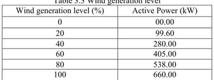
In this case study, only WTs of a size of 660 kW are considered by the DG-owning DNO even if considering different sizes simultaneously is also possible. This requirement is regulated by the accessible land for WTs’ building. The maximum generated active power by the WTs for different wind generation levels is given in Table 3.3.

Table 3.3 Wind generation level

Wind generation level (%) Active Power (kW)

0 00.00 20 99.60 40 280.00 60 405.00 80 538.00 100 660.00

The maximum number of WTs that can be allocated at a given bus is represented by an equivalent number of blocks in the WT’s offer. At each candidate bus it is assumed that maximum four WTs of each size can be allocated, thus, for each generation level there are four blocks of the same size equal to the rated power of the selected WTs and the same price of 70 €/MWh. In the following subsection, the method of calculating WT’s offer price from the point of view of DNOs is explained.

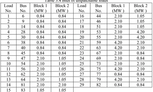
The offers are assumed at price of 120 €/MWh for the bus connecting the distribution network to the transmission one. Regarding the bids for DLs, it is assumed that there are two blocks per demand bid with different sizes as presented in Table 3.4 and the same price of 250 €/MWh for all blocks.

Table 3.4 Bids of dispatchable loads Load No. Bus No. Block 1 (MW ) Block 2 (MW ) Load No. Bus No. Block 1 (MW ) Block 2 (MW ) 1 6 0.84 0.84 16 44 2.10 1.05 2 9 0.84 0.84 17 46 2.10 1.05 3 14 0.84 0.84 18 51 2.10 1.05 4 28 0.84 0.84 19 53 2.10 4.20 5 30 0.84 0.84 20 55 2.10 4.20 6 38 0.84 0.84 21 59 4.20 2.10 7 40 0.84 0.84 22 63 4.20 2.10 8 45 0.84 0.84 23 67 2.10 0.84 9 47 2.10 1.05 24 69 2.10 0.84 10 54 2.10 1.05 25 73 2.10 2.10 11 56 2.10 1.05 26 75 4.20 2.10 12 62 2.10 1.05 27 77 0.84 0.84 13 64 2.10 1.05 28 79 4.20 2.10 14 81 2.10 2.10 29 82 0.84 0.84 15 83 1.05 1.05

3.4.1 WTs’ Offers Price Calculation from the Point of

View of DNO

In order to calculate the price of WTs’ offers, financial data, i.e. WTs’ life time, installation cost, depreciation time, interest rate, are considered as summarized in Table 3.5 [98,99]. The annual cost for WTs is calculated as follows [99]: Cost Inst i i i Cost Ann _n n _ 1 ) 1 ( ) 1 ( _      (3.16)

where i is the interest rate, n is the depreciation period in years,

Inst_Cost is the installation cost, and Ann_Cost is the annual cost for

depreciation. The capacity factor is evaluated according to the wind generation data and the WTs capability curves. For example, for a 660 kW WT the capacity factor is about 45%, i.e. 4010 MWh/MW. Therefore, by dividing Ann_Cost by equivalent number of hours i.e. 4010 h, the WT’s offer price with no subsidy is about 70 €/MWh. Therefore, the 660 kW WT’s offer price, without subsidies, is assumed as 70 €/MWh.

Table 3.5 Financial Data for Estimating WT’s Offer Price Life time (years) 20 Installation cost (€/kW) 1700 Depreciation time (years) 10

Interest rate (%) 10 Number of equivalent hours (MWh/MW) 4010

Capacity factor (%) 45 Annual cost (€/kW-year) 280 Calculated offer (€/MWh) 70

3.4.2 Simulation Results

The proposed method is applied to the abovementioned distribution network. The method has been implemented in MATLAB® incorporating some features of MATPOWER suite [93, 94].

In order to determine the optimal numbers and capacities of WTs, DNOs assume the worst-case situation of minimum load and maximum generation. When a WT operates at maximum generation and minimum load it leads, in fact, to large reverse power flows with large local voltage variations [100]. So, the mentioned case is assumed as worst-case situation. The optimal numbers and capacities of WTs are obtained in this case as provided in Table 3.6. The simulation results for different combinations of load demand and wind power generation considering the optimal number of WTs obtained in the aforementioned case, as given in Table 3.6, is shown in Figs.3.5 to 3.7.

Table 3.6 Optimal number and capacity of allocated WTs Bus No. Total capacity (MW) Number of allocated WTs

6 2.64 4 9 1.32 2 14 0.66 1 28 2.64 4 30 1.32 2 38 2.64 4 40 0.66 1 45 2.64 4 47 0.66 1 54 2.64 4 56 0.66 1 62 2.64 4 64 1.32 2 81 2.64 4 83 0.66 1 Total 25.74 39

Buses 6, 28, 38, 45, 54, 62, and 81 have the largest WT capacity (2.64 MW) while buses 14, 40, 47, 56 and 83 have the lowest ones (0.66 MW). The installed capacity of WTs is, in fact, limited by voltage and thermal limits as well as by the bids of DLs at each bus. The installed capacity at bus 40, for example, is limited to one WT. It is mainly due to the lowest value of both thermal limit of the line connecting the buses 39-40 (i.e. 40 A) and the DLs’ bids if compared to those at the other lines and buses, respectively.

At bus 64, with the higher thermal limit of the lines 63-64 connecting the buses (i.e. 50 A), and the higher bids of DLs if compared to previous case, the installed capacity is 1.32 MW corresponding to two WTs. In addition, at buses 54 and 62 the thermal limits of the lines 53-54 and 61-62 connecting the buses are 180 A and the DLs’ bids are higher if compared to previous cases. This determines that voltage and thermal limits are not binding (active) and consequently the installed capacity at these buses is 2.64 MW corresponding to four WTs.

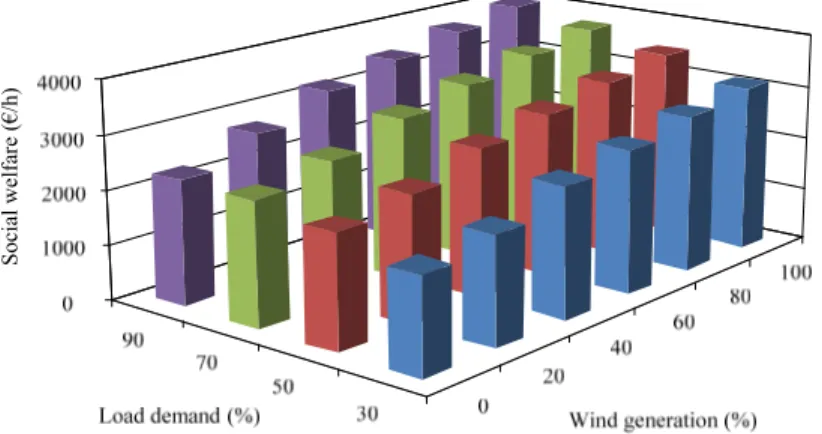
As regards with the SW, it increases proportionally to the both load demand and wind power generation as shown in Fig. 3.5. It is

worth mentioning that, in all scenarios, the SW is higher if compared to that without WTs in the network.

It is evident that in the case of minimum load, i.e. 30%, and maximum wind generation level, i.e. 100%, the SW is equal to about 3000 €/h and in the case of maximum load and minimum wind generation, the SW is equal to about 2000 €/h while in the case of maximum wind generation level and maximum load demand this value is equal to around 4000 €/h which is higher if compared to previous cases.

Fig. 3.6 shows the total dispatched active power by WTs in different scenarios of wind generations and load demands. It is seen that the dispatched active power has the direct relation with both load demand and wind power generation. In all scenarios, the dispatched active power is higher if compared to that with no WTs in the network.

The supplied loads, shown in Fig. 3.7, evidences its direct relation with wind generation and its inverse relation with load demand due to the network constraints that limit load increase when constraints are binding. It is worth pointing out that, in all scenarios, the value of supplied loads is higher if compared to that without WTs in the network.

The method is computationally very fast, i.e. it takes about 45 seconds, for all scenarios, measuring the CPU time consumption on a laptop with core i7, 1.6 GHz processor and 4 GB of RAM.

Soci al welf ar e (€ /h)

Fig.3.6. Dispatched active power

Fig.3.7. Supplied load

3.5

Distribution System Planning within

Market Environment

3.5.1

Aim and Approach

In this section, deterministic methods for optimal placement of WTs in distribution networks within a DNO acquisition market environment are proposed. The methods include: 1) hybrid GA and market-based OPF for annual energy losses minimization from the

point of view of DNO; 2) hybrid PSO and market-based OPF for NPV maximization from the viewpoint of WTs’ developers.

The uncertainty in wind power generation and load demand is modeled through hourly time-series model of load demand and wind generation. The interrelationships between demand and generation potential are preserved with their joint probability defining the number of coincident hours over the target year.

To the best of our knowledge, no wind power investment methods in distribution level in market environment by using abovementioned hybrid methods have been reported in the literature. The contributions of this section are as follows:

1) Providing a hybrid optimization method for wind power investment in distribution level by using market-based OPF and GA/PSO within a DNO acquisition market environment. Note that market-based OPF is also used to clear the DNO acquisition market. Furthermore, the DNO is the market operator of the DNO acquisition market.

2) Using the GA/PSO to choose the optimal size and the market-based OPF to determine the optimal number of WTs.

3) Modeling wind generation and load demand as well as correlation among different wind speeds through time series analysis approach.

3.5.2

Modeling of Time-Varying Load Demand and

Wind Power Generation

The planning horizon consists in a target year where the wind generation and load demand are modeled at each bus of the network through hourly time series analysis as shown in Fig.3.8. The method reduces hourly time-series data to a number of scenarios where the load demand and wind generation for every hour are assigned to a series of bins. Describing the number of coincident hours over the target year preserves the interrelationships between potential of load demand and wind power generation with their joint probability [16, 101].

In order to reduce the computational burden of a full time series analysis, wind generation and load demand are aggregated into a