Advanced stochastic local search methods for automatic design of Boolean network robots

ALMA MATER STUDIORUM

UNIVERSIT `

A DI BOLOGNA

Seconda Facolt`a di Ingegneria

Corso di Laurea Magistrale in Ingegneria Informatica

ADVANCED STOCHASTIC LOCAL SEARCH

METHODS FOR AUTOMATIC DESIGN OF

BOOLEAN NETWORK ROBOTS

Elaborata nel corso di: Intelligenza Artificiale

Tesi di Laurea di:

Lorenzo Garattoni

Relatore:

Prof. Andrea Roli

Correlatore:

Prof. Marco Dorigo

Dott. Ing. Mauro Birattari

Ing. Carlo Pinciroli

ANNO ACCADEMICO 2010–2011

SESSIONE III

KEY WORDS Boolean Networks Metaheuristics Robotics

Contents

2.3 Random Boolean Networks . . . 8

2.4 Boolean Network Design . . . 11

3 Boolean Network Robotics 15 3.1 Background Concepts . . . 15

3.1.1 Artificial Intelligence & Robotics . . . 15

3.1.2 Genetic Regulatory Networks . . . 16

3.2 Related Works . . . 18 3.3 Methodology . . . 19 3.3.1 BN-Robot coupling . . . 19 3.3.2 Design methodology . . . 20 4 Metaheuristics 23 4.1 Introduction . . . 23

4.2 Stochastic Local Search . . . 27

4.2.1 Local Search . . . 27

4.2.2 Trajectory-Based Methods . . . 31

4.2.3 Population-Based Methods . . . 39

4.3 Analysis of Algorithms . . . 42

4.3.1 Run-Time Distributions . . . 42

4.3.2 Search Space Structure . . . 44

5 Test Cases 47 5.1 Introduction . . . 47

ii 5.3 Obstacle Avoidance . . . 51 5.3.1 Task Definition . . . 51 5.3.2 Robot setup . . . 52 5.3.3 Evaluation . . . 53 5.4 Phototaxis . . . 55 5.4.1 Task Definition . . . 55 5.4.2 Robot setup . . . 55 5.4.3 Evaluation . . . 56

5.5 Results & Analysis . . . 58

6 Dynamic Tasks Learning 71 6.1 Introduction . . . 71

6.2 Task Definition . . . 72

6.3 Settings . . . 74

6.3.1 BN & robot setup . . . 74

6.3.2 Evaluation . . . 75

6.4 SLS Techniques . . . 80

6.5 Results & Analysis . . . 82

6.5.1 Algorithms comparison . . . 82

6.5.2 Analysis . . . 90

Acknowledgements

First of all, I would like to thank Andrea Roli, who has given me the opportunity to undertake this experience and for being always very kind and helpful. I thank also Marco Dorigo for giving me the possibility to work in IRIDIA and Mauro Birattari for his support. Many thanks to Carlo Pinciroli for his fundamental help. I am honored to have known you and worked with you.

I thank also the whole IRIDIA family: Alessandro, Alexander, Ali, Arne, Eliseo, Franco, Gianpiero, Giovanni, Manu, Giovanni 2, Gabriele, Michele, Vito, Tarik, Leonardo, Roman, Leslie, Mikael, Si-mon, Nithin, Rachael and Sara. Thank you for the great time we spent together.

I would like to thank my university colleague Matteo. We have been a great team during the last two years, especially in this last experience.

Many thanks to Claudia for hosting me but mostly for immediately becoming a good friend. Without you this great experience would have not been the same.

I would like to thank my parents for giving me the possibility to achieve my studies, for their continuous support in all my decisions.

Finally, thanks to all my friends for the important role they have in my life and simply for being my friends.

Chapter 1

Introduction

Humans have always been fascinated by the origins of intelligence. Several disciplines have tried to tackle the issue of what is the intel-ligence and how it can arise, from psychology to philosophy through artificial intelligence. During the history of this latter discipline, the question has gradually changed becoming: “Can machines behave in-telligently?”. In this context, besides answer to such question, one of the main goals of artificial intelligence is to build intelligent ma-chines (e.g. intelligent robots). For this purpose, two main categories of synthesis methodology can be defined: the first category involves a series of approaches based on a design of intelligent entities by hand. The main problem of this approach is that, with the increase of the system complexity, the synthesis would be too difficult to conceive by a human designer. Moreover, the basic characteristics of intelli-gent systems are the ability of adaptation and learning, which are features hard to obtain with an approach by hand. Thus, recent stud-ies have shown that, in many cases, it is preferable the employment of automatic design methodologies. Automatic processes are able to synthesize more flexible and robust entities and, in some cases, it has been shown that they can lead to innovative design solutions.

Typically, the automatic design process can be treated as a search problem based on two main components: the first is the model through which the robot behavior is represented and the second is the opti-mization algorithm that, working directly on the model, is designed to find the optimal configuration of its components.

Concerning the former aspect, several models exist but the most used so far are the artificial neural networks, usually trained by means of techniques inspired to the Darwinian evolution (e.g. genetic algo-rithms). In general, using genetic regulatory networks to model the

2 CHAPTER 1. INTRODUCTION dynamic behavior of intelligent entities brings relevant advantages: these models, created to simulate both the structure and the func-tional behaviors of cells, provide intrinsically the same basic features of adaptivity and flexibility peculiar of biological cells, which are able to react to environment stimuli maintaining their internal organiza-tion. In this context, the model employed for this work are the Boolean networks (BNs), introduced by Stuart Kauffman. The main advan-tages of BNs with respect to neural networks is their compactness and simplicity and the fact that it is possible to precisely define and study their dynamical behavior.

The heart of the automatic design methodology is the optimization algorithm employed to find the optimal setting of the model which al-low the intelligent entity, i.e. the robot, to perform a given target task. A suitable choice for the optimization algorithms can be the metaheuristic techniques, which are particularly appropriated for ex-ploring huge search spaces in a limited amount of time.

Recent works in this context have proposed a first proof of concepts of a methodology based on BNs and a basic metaheuristic technique. In particular, the choice of the simplest stochastic technique employed has been intended to reject the null hypothesis by preventing the re-sults from being affected by mechanisms algorithm dependent. In this work, developed in collaboration with the Institut de Recherches Interdisciplinaires et de D´eveloppements en Intelligence Artificielle (IRIDIA) of the Universit´e Libre de Bruxelles, we use the method-ology proposed as starting point, studying some prominent properties of the design process and proposing relevant improvements.

The main goals of the work are two: first, want to analyze some features of the automatic design process. More precisely, the work aims at studying the connection between the search process which trains the robot’s BN-based program to perform a specific task, and the trend of some properties of the network dynamic behavior. The hypothesis is that there exists a correlation between the learning trend and the value of certain features of the BN program, in particular in its dynamics. The second goal is the improvement of the methodology by means of advanced stochastic local search methods, drawing con-clusion about the characteristic of the search process that affect the results.

In order to achieve the proposed goals, the methodology is tested on three robotic applications. The first two applications involve simple target tasks so as to allow the analysis of a large amount of data dur-ing the whole traindur-ing process and investigate the prominent aspects.

CHAPTER 1. INTRODUCTION 3 During the last experiment, the most complex since it requires some form of memory to be performed, the main target is the methodology improvement through the employment of advanced stochastic local search algorithms.

The thesis is organized as follows:

In Chapter 2, we describe the model used to represent the robot behavior: Boolean networks. We focus on the most relevant aspect of the structure and the dynamics. Then we also present the state of the art concerning the automatic design procedure of BNs.

In Chapter 3, we introduce the background concepts of the work. In particular, after a brief historical overview about robotics and its connections with the automatic design of biological inspired networks (e.g. BNs) to control the robots, we present the related work and the basic methodology employed.

Chapter 4 provides a wide overview of the metaheuristic tech-niques. Moreover, we introduce some basic concepts used afterwards to perform the result analysis.

In Chapter 5 we discuss the robotic test cases. First we describe the task to be performed and the experimental settings for the training phase. Finally we analyze the results obtained focusing on the relevant properties emerging and trying to derive some considerations with a view to more complex tasks.

Chapter 6 concerns the final robotic application of the work. The target task is a form of sequence learning, which means that a form of memory is required. After the task description and the experimental settings, we describe the advanced stochastic techniques proposed in order to improve the methodology. Finally we compare the results and we draw important considerations about their analysis.

Finally, Chapter 7 draws some conclusions and gives an outlook for future works.

Chapter 2

Boolean Networks

In this Chapter we will introduce Boolean networks. In Section 2.1 we discuss some basic and general concepts and in Sections 2.3 and 2.4 we focus on more relevant aspects for this thesis: Random Boolean Networks and some important studies about the design of Boolean Networks through advanced local search methods.

2.1

Introduction

Boolean Networks (BNs) have been introduced by Stuart Kauffman in 1969 [1] as a model for genetic regulatory networks (GRN). Subse-quently, many works have been proposed in several research fields, and the community of complex systems is giving considerable attention to the BNs because of their properties which can model some aspects and mechanism of living system.

A BN is a discrete-state and discrete-time dynamical system. Its structure can be thought as an oriented graph with N nodes, each associated to a Boolean value xi and a Boolean function fi = (x1, ...,

xK) where K is the number of inputs of node i. The arguments of

the function fi are the boolean values of the nodes whose outgoing

arcs are connected to i. On this simple structure, it is possible to define the network dynamic behavior as a sequence of state updates (i.e., each node updates its own boolean value according to the value of inputs and the associated boolean function). In a given instant of time t, the state of the system is represented by the array of the N Boolean variable values s(t) = (x1(t) ,..., xN(t)). Many kinds of

dynamics and update schemes exist [2] but the most studied, and the one we consider in this thesis, is synchronous state updates of all the nodes and deterministic, i.e., the output of a boolean function is

6 CHAPTER 2. BOOLEAN NETWORKS unambiguously computed depending on its arguments. An example of states update in a simple boolean network is showed in Figure 2.1.

Figure 2.1: The table describes the dynamics of the BN showing the successor of each state.

2.2

Dynamics

BN model’s dynamics can be studied by means of usual dynamical systems methods, hence the usage of concepts such as state (or phase) space, trajectories, attractors and basins of attraction [3]. Chosen an initial state arbitrarily or randomly, depending on the specific ap-plication, the dynamics flows according to the update functions and scheme. Since the Boolean functions are deterministic, at each instant of time, the system passes from a state to its unique successor state. During its execution, a network traverses a succession of states, often called a trajectory in the state space. Furthermore, since the state space is finite (a node’s Boolean variable can assume the value zero or one therefore the state space size is 2N), the system will eventually assume a state previously encountered. Thus, a trajectory in the state space assumes this form:

• In the first phase, starting from the initial state, each state is different from all the previous ones and it will not be repeated. This states succession is called transient. It can also happen that this phase has length zero, i.e., the network does not undergo this phase.

CHAPTER 2. BOOLEAN NETWORKS 7 • Eventually, the trajectory will reach a point in which a state, or a sequence of states, will be repeated. This means that the network has reached an attractor. If the attractor consists of one state, it is called a point attractor or fixed point, whereas if it consists of two or more states, it is called a cycle attractor. The set of states that lead to an attractor is called the attractor basin.

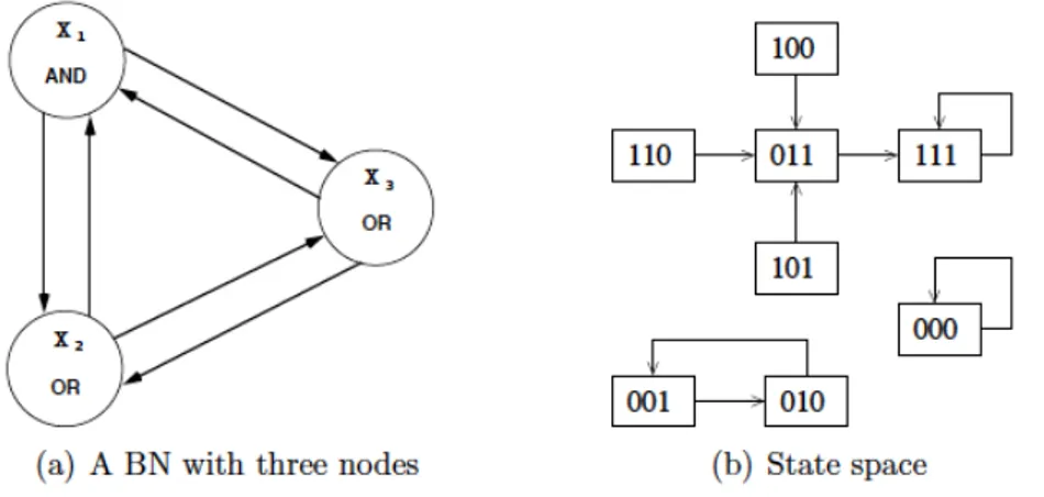
An example of a BN and its corresponding state space under syn-chronous and deterministic update is showed in Figure 2.2. Figure 2.3 shows instead the dynamics inside an attractor basin of a random boolean network.

Figure 2.2: An example of a BN with three nodes (a) and its corre-sponding state space under synchronous and deterministic update (b). The network has three attractors: two fixed points, (0, 0, 0) and (1, 1, 1), and a cycle of period 2, (0, 0, 1), (0, 1, 0).

Many dynamical features of a network can be studied such as the length of attractors or the sizes of the basins of attraction drained by the state cycle attractors. Attractors have typically been the focus of many studies because of their strong biological implications. Attrac-tors are the harbors in which the system settles down, hence they are the phase in which a system spends the most of the time. The other states in the state space are only transient points leading to such attractors. All dynamical systems, from neural networks to cardiac systems through genomic regulatory networks, exhibit attractors. For these reasons, the characteristics of attractors in system with many elements are of basic relevance in both development and evolution.

8 CHAPTER 2. BOOLEAN NETWORKS

Figure 2.3: Basin of attraction of a random boolean network with N=13 and K=3. The basin links 604 states, of which 523 are garden-of-Eden states. The attractor cycle has a period of 7

2.3

Random Boolean Networks

Random Boolean Networks (RBNs) are a special category of Boolean Networks which was also introduced by Kauffman [1] to explore as-pects of biological genetic regulatory networks. Since then, thanks to their features that capture relevant aspects and phenomena of complex systems (in particular in genetic and cellular mechanisms), they have been used as a tool in a wide range of areas such as self-organization (e.g., [5]), computation (e.g., [4]) and robotics (e.g., [16]).

Random BNs are typically created by choosing randomly K inputs per node and defining the Boolean functions assigning to each entry of the truth tables a 1 with probability p and a 0 with probability 1 -p. Parameter p is called homogeneity or bias. Depending on the value of this parameter and K we can distinguish between three different regimes: chaotic, ordered and critical. Many studies have been car-ried out about these systems regimes and the properties that a system shows during each of these regime [5]. A system is in ordered regime

CHAPTER 2. BOOLEAN NETWORKS 9 when a large part of its elements is fixed. In this kind of regime, the frozen component represents the bulk of the system and it leaves be-hind small and isolated island of components which are free to change state and have complex dynamics. On the other hand, in systems in chaotic regime, unfrozen elements form a connected component which spreads throughout the system and leaves isolated areas of frozen el-ements. The critical regime, the border between the ordered and the chaotic one, is also named edge of chaos” and it consists of an ordered sea that breaks into unfrozen islands, and the frozen islands join and percolate through the system. Many works have been proposed on the critical regime because of some its important proprieties, such as the capability of achieving the best balance between flexibility and robustness [6] and maximizing the average mutual information among nodes [7]. This features have suggested several conjectures concerning the fact that living cells, and living systems in general, are critical [8]. One of the most interesting and studied property of these dy-namical regimes is related to sensitivity to initial conditions, damage spreading, and robustness to perturbations which are different ways of measuring the stability of a network, seeing how changes affect the stable behavior. Resuming BNs, for perturbation we mean a perma-nent mutation in the connections or in the Boolean functions of the BN. A damage is instead the cascade of changes in dynamical be-havior caused by transiently altering the activity of a single binary variable [5].

In the ordered regime attractors are small and structural pertur-bations stay in small unfrozen areas, not causing cascade of damages spreading. Hence the perturbed network flows through the state space as the original one. Networks in this regime are also very robust with respect to the initial conditions whereas similar states tend to converge to the same state. In the chaotic regime, on the other hand, attrac-tors are very large and a perturbation of the activity of any single Boolean variable, causes a cascade of damage percolates through the unfrozen sea and the system. This kind of network is very sensitive to changes in initial conditions because different states tend to diverge. Finally, at the edge of chaos, perturbations can spread but damages usually remain restricted to a portion of the system. In critical net-works, moreover, nearby states tend to lie on trajectories that neither converge nor diverge in state space [9].

Living systems, and computational systems, need stability to sur-vive, but also flexibility to adapt to either the environment and the changes it could have, and explore their space of possibilities. This

10 CHAPTER 2. BOOLEAN NETWORKS has led some researchers to argue that life and computation occur nat-urally at the edge of chaos [10], or at the ordered regime close to the edge of chaos.

Living systems exist in the solid regime near the edge of chaos, and natural selection achieves and sustains such a poised state. Stuart Alan Kauffman 1993

There exist many techniques to study the features of BNs, but one of the most used is the Derrida Plot [11] which provides a measure of divergence/convergence of network dynamics in terms of Hamming distance (i.e., the number of positions at which the corresponding symbols are different) between states. In particular, in a Derrida Plot pairs of initial states are sampled at defined initial distances, H(0), from the entire state space, and their mean Hamming distance, H(t), after a fixed time, t, is plotted against the initial distance H(0). For perturbation calculation, we consider two copies of the same RBN and we flip n node values in one copy. Then, we compare the states of the normal network with the state of mutated network by means of the Hamming distance H(t), after a fixed time (i.e. after a state update of both the two networks). Repeating this procedure for different values of n between 0 and N and plotting the results, we can highlights the effect of perturbation and distinguish between ordered, chaotic and critical regime measuring the slope of the plot.

Thanks to these studies, scientists identified another important feature about dynamical regimes: changing the value of K, the dy-namic regime of RBNs changes too. In particular, networks with K ≤ 2 are in the ordered regime, and networks with K ≥ 3, are in the chaotic regime. Derrida and Pomeau were the first to determine ana-lytically that the critical phase was found when K = 2 [12]. Figure 2.4 shows dynamics of RBNs in different phases. To explain the motiva-tion of this dependency between the number of inputs of each node of the network and the dynamical regimes we need to introduce the concept of canalyzing functions. A canalyzing Boolean function is any Boolean function having the property that the output is determined by only one input (for instance one input with value 1 is enough to let the OR function assume the value 1). The consequence of having many canalyzing functions inside a network is that a node value can force the elements it regulates to assume the same value at the next moment. Such a mechanism propagated iteratively to all the descen-dants along with the fact that the network has loops, creates forcing loops or descendant forcing structures [5]. The creation of large

forc-CHAPTER 2. BOOLEAN NETWORKS 11 ing structures produces order in the network since these frozen areas form a large interconnected web that percolates through the whole system. Several works have been produced to prove the relationship between K and the number of canalyzing functions in the networks, and consequently the dynamical regimes [5].

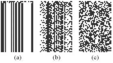
Figure 2.4: Trajectories through state space of RBNs within different regimes, N = 32. A square represents the state of a node. Initial states at top, time flows downwards. a) ordered, b) critical, c) chaotic

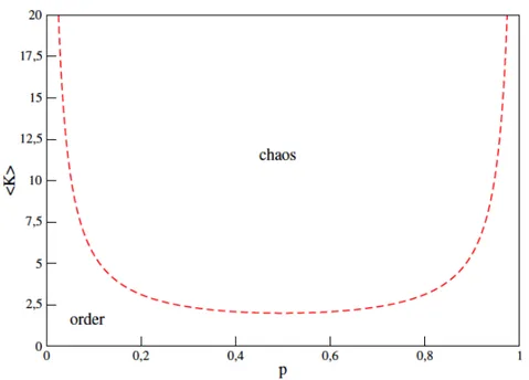
Derrida and Pomeau also introduced two important generalizations of the classical model: the first concerns nonhomogeneous networks (K is not necessarily the same for all nodes), and another is that they considered the concept of homogeneity or bias p (as mentioned above each entry of the truth table have a probability p of being one and 1 - p of being zero), to numerically find the critical line corresponding to the critical regime and to define the relation between the parameters of the networks. Thanks to these intuitions and to the method they used called Derrida annealed approximation, they defined the following equation which describes the critical line:

2p(1 - p) = 1/K (2.1) The plot of this equation can be seen in Figure 2.5.

2.4

Boolean Network Design

The design of complex systems is one of the main challenges in sci-entific and engineering disciplines. Scientists have to face this basic

12 CHAPTER 2. BOOLEAN NETWORKS

Figure 2.5: Relationship between p and K in phase transitions issue in many research areas, such as reverse engineering of biological and social networks, design of self-organizing artificial systems and robotics. One of the most widely used approaches to tackle the prob-lem is the synthesis and tuning of such systems by means of automatic techniques, most of which are search methods. Despite BNs, especially in the past, have been mainly used to model and study genetic or bi-ological phenomena, more recently, several works have been produced to explore their potential as computational learning systems. One of the main reasons to investigate the learning process of Boolean Net-works is that it is possible, in this scenario, to precisely define their dynamical state.

The first contribute concerning the potential of BNs as learning systems was by Kauffman [13], who in his work proposed a modified genetic algorithm (with only a mutation operator) with the objective of generating networks whose attractors matched a prescribed target state. Afterwards, Lemke et al. extended the scenario to cycle attrac-tors targets using a full implementation of genetic algorithm (with crossover). Those studies, and other more recent including the dis-cussion of experimental results on the application of a simple genetic algorithm to to obtain an attractor with a given length [14], are an investigation of the impact of evolution over BNs. In particular, they were meant to evolve some specific features in the networks, mostly

CHAPTER 2. BOOLEAN NETWORKS 13 structural or dynamical properties such as the length of attractors or the control of the BN’s trajectory to match a target [15]. On the other hand, few works have been proposed aimed at revealing some behavioral aspect of the network so that they can be used to address some specific task. Examples of this second approach are [15], in which the author uses the Boolean networks trained by either a Ge-netic Algorithm and a Iterated Local Search (ILS) to solve the Density classification problem, or [17] and [16] where the authors exploit a first investigation of the potential of automatic designed BN controllers for robots (we will discuss this topic in detail in the next Chapter).

The results obtained in all the mentioned studies raise interesting questions on the training algorithm, the search landscape structure and the evolutionary dynamics depending on the networks character-istics. We will focus on all these concepts in Chapter 4.

Chapter 3

Boolean Network Robotics

This Chapter introduces some basic concepts regarding the use of Boolean Networks in Robotics. In the Section 3.1 we introduce a series of background aspects required to fully understand the rise of this recent approach. In particular we give a brief historical introduction to robotics, and subsequently we illustrate the relevance of the genetic regulatory network models inside this discipline. Moreover, in Section 3.2 we present some related works and finally, in Section 3.3, we outline the automatic BN-robotic design methodology which we will use as starting point for our studies.

3.1

Background Concepts

In this section we present a historical introduction to Artificial Intel-ligence and Robotics, focusing on the aspect close to our work. In Section 3.1.2, we describe the basic features of the cellular models and the reasons for which they can be usefully employed in robotics, presenting some prominent examples of these studies.

3.1.1

Artificial Intelligence & Robotics

Humans have always been fascinated by the question about “what is intelligence”. This issue has has been tackled by several disciplines, and the debate also includes the ideas of many philosophers and psy-chologists. Since the beginning of the XX century, thanks to techno-logical advances, the question has gradually changed becoming: “Can machines think?”, that is also “Can machines behave intelligently?”. The discipline that, in the recent history, has tried to give an answer to these questions is Artificial Intelligence (AI). AI has its origin from

16 CHAPTER 3. BOOLEAN NETWORK ROBOTICS the work of Turing [18] which represented a milestone for the theory of computation and computability and was the basis for subsequent pro-gresses in the field of machine computing. Some years later, in 1956, Newell and Simon [19] presented a program that could demonstrate theorems in logic, and on the basis of this and of another work by Newell and Simon [20], in AI the physical symbol hypothesis became prominent: every intelligent behavior could be simulated by appro-priate manipulation of physical symbols. In this direction, artificially intelligent systems were built so that they could solve whatever prob-lem for which knowledge could be modeled in form of logic symbols. Even in robotics, which in the meantime had grown up also thanks to the cybernetic contribution (discipline that studied the animals as if they were machines and tried to model their behaviors using control theory and statistical information theory), reasoning was performed by symbolic manipulation of symbols. In 1980s, a new paradigm in contrast with the symbolic paradigm, connectionism, moved its first steps studying artificial neural networks (bottom-up approach). The real revolution, however, started with Brooks [21] who thought that the study of Artificial Intelligence should start from building machines that interact with the real world, abandoning the top-down traditional approach for which modeling was always required. The idea of Brooks was to turn to a biologically-oriented, bottom-up methodology. He also introduced two basic concepts for modern robotics: situatedness (i.e. robots perceive the world through their sensors, and the world provides them all the information required to execute their behavior) and embodiment (i.e. robots can act on the environment, moving in the world and modifying it, actively determining what will be the feedback they will subsequently receive). These concepts are today the basis of the design of embodied agent programs. The work of Brooks gave rise to a series of new studies about embodied cognitive science, where the importance of embodiment stems from the possibility to exploit the dynamic interactions of the agent with the environment, so that intelligent behaviors can emerge. The same ideas are also the basis of other studies, which use biological or, in general, natural inspired models and processes to synthesize robot agent programs.

3.1.2

Genetic Regulatory Networks

One of the branches of research generated by the studies presented in Section 3.1.1, concerns the exploitation of embodied Genetic Reg-ulatory Networks (GRNs) as real-time control systems for artificial

CHAPTER 3. BOOLEAN NETWORK ROBOTICS 17 organisms, in particular robots. GRNs are models used to simulate both the structure and the functional behaviors of cells. This kind of approach in robotics arose from a series of historical considerations about the concepts of embodiment and adaptivity. Maturana and Varela in 1980 [22] argued that adaptivity is not limited to a mere reaction to environmental stimuli. It takes place due to a “structural coupling” between the agent and the environment, during which they are both sources of mutual perturbations. From this point of view, the cognition of an agent is considered as “functional embedding” of an agent in its interaction with the world. This kind of embodiment considers adaptation as the capability of an agent to maintain its in-ternal organization in relation to the perturbations that come from the environment. In Maturana and Varela’s view [22], this features of maintaining under control the internal organization is peculiar to living systems and cannot be found in artificial artifacts. The basic ex-amples of such adaptivity property in living systems is the biological cell: it is composed by several parts enclosed within the cell mem-brane. All these parts are connected to form a network of interactions meant to maintain the cell internal organization.

Embodied genetic regulatory network-driven control systems ex-ploit this natural metaphor to develop flexible and robust controllers, able to dynamically adapt to the environment and continually driving the interplay between agent and environment, giving rise to coherent observable emergent behaviors. The GRN model most commonly used so far are neural networks, models that attempt to simulate either the structure or functional aspects of the biological central nervous sys-tem. Nevertheless, several GRN models have been proposed like the Biosys model used in [23], in which a cell consists of Genes and Pro-teins that regulate the interaction of the cell with the environment. Another important model are the Boolean networks, the model we use in the thesis which is recently having considerable consideration from the scientist thanks to the structural simplicity but in the meantime the dynamical richness.

In GRN-driven controllers, behaviors are not directly specified but rather GRNs encode complex dynamics through which structured be-haviors can emerge. In such a way, the agent (the robot in our context) performs autonomously the specific task. In particular, the GRN is continually coupled to the agent’s environment, perturbing and being perturbed, acting as a real-time control system: at each control step, first, the sensors values are encoded in the input subset of the network. Then a network update occurs. Finally the effector on the environment

18 CHAPTER 3. BOOLEAN NETWORK ROBOTICS are performed through the actuators according to the GRN’s output. The way in which the agent behaves in the environment determines the stimuli it will receive as input in the future. Moreover, it is not unusual that the interaction between the system and the environment is not perfectly known in advance.

Thus, for all the above reasons, it appears preferable to use an automatic technique, such as an optimization algorithm or an evolu-tionary algorithm, that gradually builds up the GRN control system of an autonomous agent. In order to do this, the automatic procedure exploits the behavior of the system embedded in its environment and the variations in the interactions between the environment and the agent itself. In addition, automatic design procedures can make the process simpler, more robust and general with respect to a customized procedure. The space of solutions explored by automatic technique can be larger and less constrained than that explored by conventional engineering methods. It has been shown that this feature can lead the search process to innovative design solutions [24, 25].

One of the most important example of the automatic design method-ology is Evolutionary Robotics (EV), that is a methodological proce-dure to automate the design of agent programs inspired by the winian theory of natural selection. The first intuition that the Dar-winian evolution could be used to generate efficient control systems was by Alan Turing in 1950s, when he suggested that intelligent ma-chines capable of adaptation and learning would be too difficult to conceive by a human designer. They could rather be obtained by means of an evolutionary process with mutations and selective repro-duction of the fittest individuals in a population [26]. Historically the agent program model most commonly used in the EV approach are Artificial Neural Networks [27, 28] but, in this thesis, we want to further investigate the potential of Boolean Networks as real-time robotics controller combined with the exploitation of advanced search strategies.

In the following we present some related works about this branch of research, and the description of the methodology used to automate the design process.

3.2

Related Works

The employment of the Boolean Networks in robotics is a recent pro-posal. Few studies have been presented and the one we focus on is the

CHAPTER 3. BOOLEAN NETWORK ROBOTICS 19 thesis [17] and the subsequent paper [16]. These works can be con-sidered the first attempt to automatically synthesize Boolean network robotic controllers by means of a methodological procedure. Through the new methodology proposed in this studies, which we will describe in Section 3.3, the authors were able to prove the possibility to train and tune, with a simple search algorithm, a BN controller. After the training process, the robot could manage either some simple tasks, like a path follower, or more complex tasks like phototaxis and anti-phototaxis. However, the goal of those works was to provide a proof of concept, without focusing on properties of the methodology, such as its success rate on robotics case studies and the possible improvements, or on the features that the training process arises in the network struc-ture and dynamics. This thesis aims to investigate in a deeper way the first of the two aspect just mentioned, that is the learning process improvement in terms of methodology enhancement and employment of more sophisticated search strategies. The work developed in paral-lel by M. Amaducci [29] has the goal of study the second issue, i.e., the consequences of the training process on the network dynamics and other interesting properties, like the memory representation, that can emerge from the whole process.

3.3

Methodology

In this section we describe the main aspects of the automatic design methodology for BN robot controllers proposed in the work discussed above and used in the thesis as starting point for subsequent improve-ments and inspirations.

3.3.1

BN-Robot coupling

The first thing required to the process concerns the definition of a coupling between the BN controller and the robot. In other words, we define a mapping between the robot’s sensors and the network’s input and between the robot’s actuator and the network’s output. Thus, the Boolean value of the network’s input nodes is not determined by the network dynamics but is set according to the robot’s sensor readings. Similarly, the output node values are set by the network dynamic and are used to encode the actuators activation. The mechanism is a first distinctive aspect of this approach with respect to most of the studies proposed regarding BNs, in which they have been mainly considered

20 CHAPTER 3. BOOLEAN NETWORK ROBOTICS as an isolated systems, as they have been not assumed to have inputs. Figure 3.1 shows the scheme of the coupling between BN and robot.

Figure 3.1: The coupling between BN and robot.

Several ways of defining the mapping are possible, but the most natural is via a direct encoding. In the Boolean Network model the nodes can assume only binary values. The sensor’s values and the actuator’s activation thresholds have therefore to be discretized and represented in a binary form in order to be encoded on the correspond-ing set of network nodes. This last aspect is maybe the main drawback of BNs with respect to other models because a binary encoding is not always feasible or simple in general, while in other continuos values models, like the Neural Networks, the same issue does not exist.

Once the input and the output mapping are defined, the Boolean Network, that is the robot controller, has to be designed in order to obtain a program which can perform a given task. Many approaches can be adopted to achieve this goal, such as designing a BN focusing on its dynamics properties so that they can be mapped into given features of the target robot behavior. Our methodology, instead, models the BN design process as a search problem, in which the objective function to be maximized is the robots performance.

3.3.2

Design methodology

Treating the design process as a search problem, the automatic de-sign methodology is composed by two main components: the robot program or controller and the optimization algorithm. In the matter of the robot program, we already discussed its nature: the process

CHAPTER 3. BOOLEAN NETWORK ROBOTICS 21 starts from a RBN, whose parameters are the number of input of each node K and the bias p. Both the topology and the Boolean functions are randomly generated, but while the topology does not change, the truth tables are the subject of the optimization algorithm’s moves.

Figure 3.2: Methodology approach

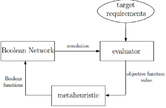
The process, which can be modeled as a constrained combinato-rial optimization problem, consists of a series of iterations whose cycle can be depicted like in Figure 3.2. At each iteration the optimiza-tion algorithm (in our case a metaheuristic technique) operates on decision variables which encode Boolean functions of the BN. The ob-tained network is then injected” into the robot (according to a suitable input-output mapping defined as described in Section 3.3.1) and exe-cuted. The resulting robot behavior is evaluated according to specific target requirements, dependent on the task to be performed. Hence, the objective function is represented by the performance measure of the robot. Typically, the execution on the real robots during the train-ing process is too expensive in terms of time and resources such as the battery charge. For these reasons, both the execution and the evalua-tion of the robot behavior are performed in a simulated environment by a specific software component. In particular, for all the robotics applications in this thesis, we use an open source modular multi-robot

22 CHAPTER 3. BOOLEAN NETWORK ROBOTICS simulator called ARGoS [31] (Autonomous Robots Go Swarming). Fi-nally, the performance evaluation is passed back to the metaheuristic technique which can thus proceed with the search process, appropri-ately modifying the BN’s Boolean functions. This process ends when a certain number of iterations is reached or when a certain target per-formance is obtained. In Chapter 5 and 6, during the presentation of the robotics experiments, we will discuss in detail all the aspects of the process.

The employment of metaheuristics ensures numerous advantages, like the efficient exploration of huge search spaces or the possibility to incrementally improve the process, starting from a simple strategy to a more sophisticated one. However, all the features of metaheuristics will be widely discussed in the next Chapter. Obviously the method-ology is not limited to the Robotics field, but it is sufficiently abstract to be employed for several other problems and disciplines.

Chapter 4

Metaheuristics

In Chapter 3 we introduced the automatic design methodology that is the basis of our synthesis process of Boolean Network agent programs. The procedure is strongly based on the metaheuristic techniques which are responsible of the search space exploration. The goal of this Chap-ter is to provide a wide panoramic of the metaheuristics, focusing on the features that make them particularly appropriated for tackling the issue of automatic design of BNs.

In Section 4.1 we give a brief introduction of the topic with some background concept, such as combinatorial problem and computa-tional complexity. Then, in Section 4.2 we introduce the stochastic local search methods, starting from the basic local search techniques and then describing more advanced local-search based and popula-tion based algorithms. Finally, in Secpopula-tion 4.3 and 4.4 we focus on some relevant properties of the result analysis and of the search space structure.

Throughout the Chapter we follow the approach of Hoos and Stut-zle in [32].

4.1

Introduction

Combinatorial problems are mathematical problems whose solutions typically consist of grouping, ordering or assignments of a discrete, fi-nite set of objects that satisfy certain conditions or constraints. Com-binations of these objects form the potential solutions of the com-binatorial problem. Prominent examples of such problems, such as finding the shortest path on a graph or determining whether there is an assignment of truth values of a logic formula under which the for-mula is satisfied, can be found in many areas of computer science and

24 CHAPTER 4. METAHEURISTICS other disciplines. It is possible to distinguish between two concepts: a problem is the abstract definition of a category of problems such as the examples cited above. A problem instance, instead, consist of a specification of all the parameters and constraints of the problem. An abstract problem can be seen as the set of all its instances. For each instance, combinations of variable values form the set of potential so-lution, namely candidate solutions. Candidate solutions are solutions that may be possibly encountered during an attempt to solve the given problem, but unlike solutions, they may not satisfy all the constraints of the problem definition. Combinatorial problems can be subdivided in two categories:

• Decision Problems: the solution of each instance of a decision problem is specified by a set of logical conditions. Two variants are possible:

– the search variant, whereby, given a problem instance, the objective is to find a solution (or to determine that no so-lution exists);

– the decision variant, in which for a given problem instance, one wants to answer the question whether or not a solution exists.

However, the two variants are related because the algorithms used to solve the search variants are also able to solve the de-cision variant. For many combinatorial dede-cision problems, the converse also holds: algorithms for the decision variant of a prob-lem can be used for finding actual solutions.

• Optimization problems: optimization problems can be seen as a generalization of decision problems, with the addition of a solution quality evaluation through an objective function. De-pending on whether this function has to be minimized or max-imized, the problems can be stated as minimization or maxi-mization problems. We can distinguish between two variants of optimization problems as well:

– the search variant, whereby, given a problem instance, the objective is to find a solution with optimal (minimal or maximal) objective function value.

CHAPTER 4. METAHEURISTICS 25 – the evaluation variant, in which for a given problem in-stance, the objective is to find the optimal objective func-tion value (i.e., the solufunc-tion quality of an optimal solufunc-tion). The search variant is the most general of these, since with the knowledge of an optimal solution, the evaluation variant can be solved trivially.

Often, optimization problems are defined based on an objective function and a set of logical conditions. In this cases candidate solu-tions satisfying the condisolu-tions are called feasible or valid, and among those, the optimal solutions can be distinguished on the basis of the objective function evaluation.

With respect to these definitions, the problem of automatic design of a Boolean network-based program for robots can be modeled as a combinatorial optimization problem, by properly defining the set of decision variables, constraints and the objective function.

The most natural way to solve a combinatorial decision and opti-mization problem is to explore and search for solutions in the space of its candidate solutions. Thus, these problems are sometimes also called search problems. Unfortunately, given a combinatorial problem instance, the size of the set of candidate solutions grows exponentially with the size of that instance. This issue raises questions about the ex-istence of efficient methods to explore such vast spaces and, specially, the time required for solving an instance of a combinatorial problem. Questions like these are the core of the computational complexity theory, that studies the classification of computational problems, in terms of computation time and memory space required to be solved. Such theory plays a fundamental role in the metaheuristic algorithms, because the primary field of application of such techniques is a class of computationally very hard combinatorial problems, for which no efficient algorithms are known (where efficient means polynomial run-time w.r.t. instance size). Complexity theory usually deals with prob-lem classes rather than the single instances. For a given algorithm, the complexity is characterized by the functional dependency between the size of an instance and the time and space required to solve this instance. Since generally the time complexity is the most restrictive factor, problems are often categorized into complexity classes with respect to their asymptotic worst-case time complexity. Thus, the complexity of a problem is usually defined by the worst-case, i.e., the time complexity in the worst case over all problem instances of a given

26 CHAPTER 4. METAHEURISTICS size. If a suitable definition of the computational complexity of an al-gorithm for a specific problem is given, the complexity of the problem itself can be defined as the complexity of the best algorithm for this problem.

Two particularly interesting complexity classes are P and N P. P is the class of problems that can be solved by a deterministic machine in polynomial time. In this definition, deterministic machine means a machine model whose decisions can be determined unambiguously, basing on its current internal state. On the other hand, N P is the class of problems that can be solved by a nondeterministic machine in polynomial time. Given the current state, nondeterministic machines make decisions choosing among a set of all the possible alternatives. They are not equivalent to machines that make random choices but rather they are idealized models of computation that have the ability to make perfect guesses for certain decisions.

Every problem in P is also contained in N P, because it is always possible to emulate deterministic calculations on a nondeterministic machine. As of today, the reverse, that is whether N P ⊆ P, and consequently P = N P, is not true because a lot of relevant problems are in N P, but they are not contained in P. This means that no polynomial-time deterministic algorithm is known to solve such com-putationally hard problems because the best algorithms known so far have exponential time complexity. This question, however, is one of the most open problems in computer science. Many of the hard prob-lems in N P are strictly related and can be translated into each other with polynomial deterministic time methods (polynomial reductions). If given a problem, every problem in N P can be polynomially reduced to it, then the problem is N P-hard and we say that it is at least as hard as any other problem in N P. This definition means that N P-hard do not necessarily have to belong to the class N P themselves, as their complexity may be higher than N P problems. N P-hard prob-lems that are contained in N P are called N P-complete: N P-complete problems are believed to have at least exponential time-complexity for any realistic machine or programming model; in a certain sense, these problems are the hardest problems in N P.

One fundamental result of computational complexity theory states that it suffices to find a polynomial time deterministic algorithm for one single N P-complete problem to prove that N P = P. This stems from the fact that all N P-complete problems can be encoded into each other in polynomial time.

CHAPTER 4. METAHEURISTICS 27 Despite many practical relevant combinatorial problem are N P-hard or N P-complete, this does not mean that that it is impossible for a problem to be solved efficiently. We can distinguish between two main possible approaches to solve these kind of problems:

• Complete techniques: they are guaranteed to return an op-timal solution in finite time, or return failure if the problem is infeasible, for every finite size instance of a problem. The draw-back is that for growing problem size, the problem instances be-come quickly intractable in terms of computation time needed for practical purposes.

• Approximate Techniques: they do not return proof of opti-mality but they find (near-)optimal solutions efficiently, signifi-cantly reducing the complete algorithms amount of time. In Section 4.2 we discuss the general approach of approximate al-gorithms, which can be characterized as search algorithms. We will focus on advantages and disadvantages of these techniques, highlight-ing the reasons of the introduction of more sophisticated algorithms, the metaheuristics.

4.2

Stochastic Local Search

All the common approaches for solving hard combinatorial problems can be characterized as search algorithms. The basic idea behind these algorithms is to iteratively generate and evaluate new candidate so-lutions. Evaluating a candidate solution means to decide whether it is an actual solution in the case of combinatorial decision problems, while it means determining the respective value of the objective func-tion in the case of optimizafunc-tion problems. Despite the time complexity of N P-hard problems is exponential, search algorithms can be much more efficient, i.e. characterized by polynomial complexity. Moreover, the evaluation of candidate solutions is often rather straightforward to implement.

4.2.1

Local Search

Search methods can be classified on the basis of different aspects, mainly the way in which the candidate solutions are generated and the search space visiting paradigm. The most common distinction,

28 CHAPTER 4. METAHEURISTICS based on the second aspect, is between systematic and local search: systematic search algorithms traverse the search space completely, en-suring that eventually either a solution is found (if it exists), or the fact that no solution exists for the problem instance is determined with certainty. This property of systematic search algorithm is called com-pleteness. On the other hand, local search algorithms start at some location of the search space, representing a feasible solution, and try to improve it by iteratively move from the present location to a neigh-boring location. Each location in the search space has a relatively small number of neighbors and the moves are performed on the basis of decision based on local information only. This kind of algorithms are typically incomplete, which means that it is not guarantee that existing solutions are eventually found, and if no solution exists, this fact will never be determined with certainty.

Local search algorithms are often based on perturbative search: candidate solutions are composed of solution components, such as the values in the Boolean functions of a Boolean network during a learning process. Therefore, given a candidate solution it is easy to move to a new candidate solution, that is a neighbor for the first one, modifying one or more of the corresponding solution components. These small local modifications can be characterized as perturbations of the current candidate solution. Hence, the methods based on this space navigation mechanism can be classified as perturbative search methods.

Other local search algorithms, characterized as constructive search methods, use a different approach: these algorithms try to generate “good” (where for optimization problems, the goodness corresponds to the value of the objective function) complete candidate solutions by iteratively extending partial candidate solutions. In many cases constructive local search methods can be combined with perturba-tive local search exploiting the advantages of an hybrid approach. Moreover, both perturbative and constructive methods combined with other mechanisms such as the backtracking, can be the basis of sys-tematic search methods.

According to the foregoing discussion, it might be argued that, due to their incompleteness, the local search techniques are generally inferior with respect to systematic algorithms. But this is not the case, because there are many problem instances which are known to be solvable, and hence in these situations the goal is to find a solution rather than understand whether one exists. In addition, in scenarios in which the time to find a solution is limited, that is almost every real world problem, systematic algorithms may need to be stopped

CHAPTER 4. METAHEURISTICS 29 before the search termination. This premature termination can cause problems, specially to the constructive techniques that search through spaces of partial solutions without computing complete solutions early in the search. Thus, local search algorithms are often advantageous in certain situations, particularly if reasonably good solutions are re-quired within a short time, if parallel processing is used and if the knowledge about the problem domain is rather limited.

Many of most widely used and successful local search algorithms exploit the use of randomized choices in generating or selecting can-didate solutions for a given problem instance. These algorithms are called Stochastic Local Search (SLS) methods. As discussed above, the search process starts from a selected initial candidate solution and then proceeds by iteratively move from a position to a neighbor-ing candidate solution, makneighbor-ing decisions on the basis of limited local knowledge only. In SLS methods, these decisions as well as the search initialization can be randomized. In addition, the search process may use additional memory, for instance, for storing a limited number of recently visited candidate solutions.

In order to formally describe a stochastic local search process for combinatorial problems, we need to define some basic components which provide the basis for solving a given problem using the SLS paradigm:

• The search space S(π) of instance π, which is a finite set of candidate solutions s ∈ S (also called search positions, locations, configurations or states); over this space it is also defined a set of (feasible) solutions S’(π) ⊆ S(π);

• A neighborhood structure is a function N : S → 2S _{that assigns}

to every s ∈ S a set of neighbors N (s) ⊆ S. N (s) is called the neighborhood of s. Typically, the choice of an appropriate neigh-borhood relation is fundamental for the performance of an SLS algorithm and often, this choice needs to be problem specific. • An objective function f(π,s): S(π) → R that maps each search

position onto a real number in such a way that the global optima of π correspond to the solutions of π. The objective function is used in the search process to assess the candidate solutions in the neighborhood of the current position. Thus the objective func-tion guides the search process, and the efficacy of the search de-pends on its properties. For these reasons this function is usually problem-specific and often depends on the search space, solution

30 CHAPTER 4. METAHEURISTICS set and neighborhood underlying the SLS. Notice that often a distinction is drawn between the concept of evaluation function (denoted with g and used to assessing or ranking candidate so-lutions in the neighborhood of the current search position) and the objective function f. The objective function characterizing the problem is often used as an evaluation function, such that the values of the evaluation function correspond directly to the quantity to be optimized. Thus, in the following we do not use this distinction, simply using the concept of objective function f (for completeness, in the figures that outline the algorithms such distinction is maintained).

• A finite set of memory states M(π), which, in the case of SLS algorithms that do not use memory, may consist of a single state only.

• An initialization function init(π) which specifies a probability distribution over initial search positions and memory states. • A step function step(π) that map each search position and

mem-ory state onto a probability distribution over its neighboring search positions and memory states.

• A termination condition which indicates the probability with which the search is to be terminated upon reaching a specific point in the search space and memory state.

The metaheuristic search can be thought as a search process over a graph characterized by the triple L = (S, N , f ), that is the solution set, the neighborhood function and the objective function. The search starts from an initial node and explores the graph moving from a node to one of its neighbors, until it reaches the termination condition.

One of the most basic examples of SLS techniques is the iterative improvement. Iterative improvement starts from a randomly selected point in the search space (all the position in the search space have the same probability to be chosen), and then tries to iteratively improve the current candidate solution with respect to the objective function f. A move is only performed if the candidate solution it produces is better than the current solution. A stochastic version of this algorithm also exists, called Stochastic Descent (SD), in which the neighbor to be evaluated is randomly picked into the neighborhood sets.

Note that, following the definition of iterative improvement, in the case in which none of the neighbors of a candidate solution s

CHAPTER 4. METAHEURISTICS 31 realizes an improvement, the search process terminates even if the quality of the current solution is not satisfying. A candidate solution with this property corresponds to a local minimum of the objective function f. A locally minimal solution (or local minimum) can be formally defined with respect to a neighborhood structure N as a solution ˆs such that ∀ s ∈ N (ˆs) : f (ˆs) ≤ f (s). We call ˆs a strict locally minimal solution if f (ˆs) < f (s) ∀ s ∈ N (ˆs). In cases where an SLS algorithm guided by an objective function encounters a local minimum that does not correspond to a solution, this algorithm can “get stuck” so that it can not find good solutions. For these reasons the basic techniques have been extended and enhanced with strategies that are required to prevent the search from getting trapped in local minima and to escape from them. In the following we present some of the most known SLS algorithm, describing the escape strategies and the advantages of each one, deepening more in those related to the thesis. SLS methods can be usually classified into trajectory methods, and population-based methods. The former kind describes a trajectory over a search graph while the latter methods perform a search process characterized by an iterative sampling of the search space. We apply the same classification in our following discussion.

4.2.2

Trajectory-Based Methods

Introducing the iterative improvement we highlighted its main lim-itation, i.e. the fact that it can get stuck in local minima of the underlying objective function. The first simple idea that can alleviate this problem is using a larger neighborhood. As discussed before, the performance of a search method significantly depends on the neighbor-hood relation definition, in particular, on the size of the neighborneighbor-hood. Generally, larger neighborhoods contain more and potentially better candidate solutions, and hence they typically offer better chances for finding locally improving search steps. Clearly, the time complexity for determining improving search steps is much higher in larger neigh-borhoods. In this context, there is a tradeoff between the benefits of using large neighborhoods and the associated time complexity of performing search steps. One possible way to partially solve this is-sue is to use a neighborhood pruning method. This kind of approach consist in using large neighborhoods but reducing their size by never examining neighbors that are unlikely to yield any improvements.

32 CHAPTER 4. METAHEURISTICS First Improvement & Best Improvement

Another simple method for making the local search technique more efficient is to select the next search step more efficiently. From this perspective, the Iterative Best Improvement method is based on the random selection, at each step, of one of the candidate solutions that achieve a maximal improvement in the objective function. One thing to notice is that this algorithm, also known as greedy hill-climbing or discrete gradient descent, needs a complete evaluation of the whole neighborhood in each step.

The Iterative First Improvement algorithm tries to avoid the time complexity of evaluate all neighbors at each search step, selecting the first improving candidate solution encountered during the neighbor-hood evaluation process. Obviously, the order in which the neighbors are visited during the evaluation, can deeply affect the performance of this strategy. Instead of using a fixed order, random orderings can also be used.

Summarizing, the search steps in first improvement algorithms can often be computed more efficiently than in best improvement, since typically only a small part of the local neighborhood is evaluated. However, the improvement obtained by each step of first improve-ment is usually smaller than for best improveimprove-ment and therefore, more search steps have to be performed in order to reach a local optimum. Variable Neighborhood Search

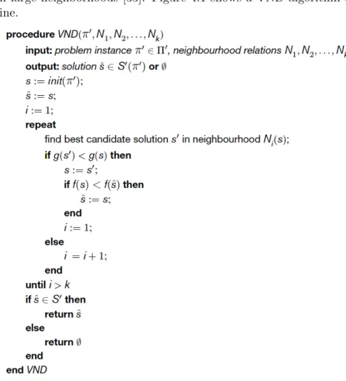
Resuming the idea of larger neighborhood to increase the search pro-cess performance, another common approach can be exploited. It consists of using standard neighborhoods until a local minimum is encountered, at which point the local search switches to a different, typically larger, neighborhood, which may allow the process to es-cape from the local minimum and reach further progress. This idea is the basis of the Variable Neighborhood Search (VNS) framework, which comprises a number of algorithmic approaches including Vari-able Neighborhood Descent (VND). VND is an iterative improvement algorithm that realizes the general idea behind VNS in a very straight-forward way. In VND, k neighborhood relations are defined which are often ordered according to increasing size: |N1| < |N2| < . . . <

|Nk max | . During the search process, the algorithm switches to

neigh-borhood structure Ni to Ni+1 whenever the search stagnates, that is

whenever no further improving step is found for a neighborhood Ni.

CHAPTER 4. METAHEURISTICS 33 to N1, from where the process is continued as previously described.

It has been shown that variable neighborhood descent can consider-ably improve the performance of iterative improvement algorithms. Such improvements are both w.r.t. to the solution quality of the local optima reached, as well as w.r.t. the time required for finding (high-quality) solutions compared to using standard Iterative Improvement in large neighborhoods [33]. Figure 4.1 shows a VND algorithm out-line.

Figure 4.1: Algorithm outline for Variable Neighborhood Descent for optimization problems

A different approach to the idea of larger neighborhood concerns the selection of search steps from large neighborhoods efficiently, com-posing more complex steps from a number of steps in small and sim-ple neighborhoods. The idea is exploited in Variable Depth Search (VDS) and in Dynasearch. The former can be seen as an iterative im-provement method in which the local search steps are variable length

34 CHAPTER 4. METAHEURISTICS sequences of simpler search steps in a small neighborhood. The lat-ter, differently from VDS, requires that the individual search steps that compose a complex step are mutually independent. Indepen-dence means that the individual search steps do not interfere with each other with respect to their effect on the objective function values and the feasibility of candidate solutions.

Randomized Iterative Improvement

Another idea to let the search out from local minima is to accept that in some cases the search process can perform worsening steps which can help to escape. One of the simplest ways of exploiting this idea is to extend iterative improvement algorithms such that they select, sometimes, a neighbor at random rather than an improving move. The alternation with a fixed frequency of such random walk steps and im-provement steps can lead to situations in which the effect of a random selection are immediately undone by the subsequent improvement se-lection. In order to avoid the problem, it is possible to introduce a parameter wp ∈ [0,1], called walk probability or noise parameter, that corresponds, at each step, to the probability of performing a random move rather than a improvement move. The resulting algorithm is called Randomized Iterative Improvement (RII). It differs from a it-erative improvement just for two aspects: the step function, in which it determines probabilistically the step to be executed, and for the termination condition, because there is no more need to terminate as soon as a local optimum is encountered.

An advantageous consequence of the fact that arbitrarily long se-quences of random steps can occur is that there is always a chance to escape from any local optima. However, RII is rarely applied in prac-tical application, probably due to the fact that more complex SLS algorithms can often achieve better performances.

Simulated Annealing

Simulated Annealing (SA) is a SLS that explores a similar idea: the probability of accepting a worsening step should depend on the value of the objective function such that the worse a step is, the less likely it would be performed. This idea is the basis of a family of algo-rithms called Probabilistic Iterative Improvement (PII). In these tech-niques each step can be split into two stages: in the first, a neighbor of the current candidate solution is randomly chosen. In the second stage, an acceptance criterion is applied, according to a probability

CHAPTER 4. METAHEURISTICS 35 distribution over neighboring candidate solutions based on their re-spective objective function value. The acceptance criterion, known as the Metropolitan condition, is shown in Figure 4.2.

Figure 4.2: Acceptance criterion in simulated annealing

The probability of performing worsening steps depends on the pa-rameter T, also called temperature. The higher the temperature is, the more likely the algorithm is to accept even drastically worsening steps with relatively high probability. Maintaining the temperature constant during the search, we obtain a PII algorithm while the pe-culiarity of the SA is exactly the generalization of this idea: T can vary over the search process through a mechanism called annealing schedule or cooling schedule inspired to the physical annealing pro-cess. An annealing schedule is a function which determines, at each instant of time t, the respective value of temperature T(t). There exist several ways to vary the temperature during the search, such as geo-metric, logarithmic or non-monotonic. The choice, obviously, strongly depends on the problem to be solved but the simple geometric cooling schedule has been shown to be quite efficient in many cases.

Simulated annealing is one of the most used algorithms. The rea-son can be the fact that it is simple to enhance it with other techniques such as a greedy initialization or neighborhood pruning. Another ap-pealing reason can be the fact that, under certain conditions, the convergence of the algorithm can be proven (i.e., any arbitrary long trajectory in the search space is guaranteed to terminate in an optimal solution). The conditions are, however, extremely severe and typically not feasible in practical applications.

Tabu Search

A radically different approach to tackle the problem of escaping from local minima exploits information about the search history. Tabu Search (TS) is a general SLS method that systematically utilizes mem-ory to guide the search process. In particular, we focus on the sim-plest and the most widely used technique, also known as simple tabu search. It uses a short-term memory in order to both avoid cycles

36 CHAPTER 4. METAHEURISTICS in the search trajectory and to escape from local minima. Typically, simple tabu search consists of a best improvement strategy to select the best neighbor of the current candidate solution. In a local mini-mum, this can lead to a worsening step or to a plateau step (i.e., a step which does not lead to any change in the objective function value). In order to prevent the search process to immediately return to a previ-ously visited neighbor, TS keeps track of recent visited solutions and forbids them. Often, memorizing solutions is not convenient in terms of performance, therefore moves, i.e. solutions components, are stored instead. However, storing moves instead of solutions could forbid im-proving, not yet visited candidate solutions. For this reason, many TS algorithms use an aspiration criterion, which specifies the conditions under which a tabu restriction is overridden, thereby including the otherwise forbidden solution. A commonly used aspiration criterion is to allow solutions which have improving evaluation with respect to the currently-known best solution.

The most important parameter of TS is the the duration (in search steps) for which the tabu restrictions is applied, called tabu tenure. If tabu tenure is too small, search stagnation may occur. If it is too large, the search trajectory is restricted and good solutions may be missed. More complex version of the algorithm exist, that try to find a tabu tenure optimal value in different ways or extend the memory to form of intermediate-term or long-term memory.

Tabu search algorithms have been successfully applied to several combinatorial problems. Often, beyond the tabu tenure value, a care-ful choice of the neighborhood definition is crucial for the performance of these algorithms.

Dynamic Local Search

The previous techniques exploit two main strategies to guide the search process out from local optima: the first allows worsening steps while the second concerns changing the neighborhood structure during the search. We can account into the latter the variable neighborhood search algorithms, which increase the neighborhood size, and the tabu search methods, which instead change the neighborhood structure for-bidding certain movements.

A further idea is to modify the search space with the aim of mak-ing unexplored areas more desirable. In order to do that, the SLS algorithms collectively called Dynamic Local Search (DLS) methods, change the objective function dynamically whenever a local optimum