Improving Deep Question Answering: The ALBERT Model

Alma Mater Studiorum

· Università di

Bologna

SCUOLA DI SCIENZE

Corso di Laurea Magistrale in Informatica

IMPROVING DEEP

QUESTION ANSWERING:

THE ALBERT MODEL

Relatore:

Chiar.mo Prof.

FABIO TAMBURINI

Correlatore:

Chiar.mo Prof.

PHILIPP CIMIANO

Presentata da:

MATTEO DEL

VECCHIO

Sessione III

Anno Accademico 2018/2019

“The computer is incredibly fast, accurate, and stupid. Man is

incredibly slow, inaccurate, and brilliant. The marriage of the

two is a force beyond calculation.”

− Leo M. Cherne

To my grandparents

To my family

To my friends

Sommario

L’Elaborazione del Linguaggio Naturale, o Natural Language Processing (NLP), è un settore dell’Intelligenza Artificiale che si riferisce all’abilità dei computer di capire il linguaggio umano, spesso in forma scritta e principal-mente usando applicazioni di Machine Learning e Deep Leaning per estrarre pattern. In modo più specifico, due sottoinsiemi principali sono Natural

Lan-guage Understanding (NLU) e Natural LanLan-guage Generation (NLG). Il primo

permette alle macchine di capire un linguaggio, mentre il secondo permette loro di scrivere usando quel linguaggio. Tale settore è diventato di particolare interesse a causa dei progressi fatti negli ultimi anni, in seguito all’affermarsi di nuove tecnologie, quali nuove GPU più performanti, le Google Tensor Processing Units (TPUs) [11], nuovi algoritmi o altri migliorati.

L’analisi delle lingue è molto complessa, a causa delle loro differenze, astrazioni ed ambiguità; di conseguenza, la loro elaborazione è spesso molto onerosa, in termini di modellazione del problema e di risorse. Individuare tutte le frasi in un testo è qualcosa che può essere messo in pratica con poche righe di codice, ma capire se una data frase è sarcastica o meno? Ciò è qualcosa di difficile anche per gli umani stessi e quindi richiede meccanismi molto complessi per essere affrontato. Questo tipo di informazione, infatti, pone il problema di una rappresentazione che sia effettivamente significativa. La maggior parte del lavoro di ricerca riguarda il trovare e capire tutte le caratteristiche di un testo, in modo tale da poter sviluppare dei modelli sofisticati che affrontino problemi quali la Traduzione Automatica, il Rias-sumere ed il Question Answering.

Questa tesi si concentrerà su uno dei modelli allo stato dell’arte recen-temente reso pubblico e ne approfondirà le performance sul problema del Question Answering. Inoltre, verranno mostrate alcune idee per migliorare tale modello, dopo aver descritto i cambiamenti importanti che hanno per-messo il training ed il fine-tuning di grandi modelli linguistici.

In particolare, questo lavoro è strutturato come di seguito:

• Il Capitolo 1 contiene un’introduzione sulle Reti Neurali, il loro uso e il ruolo che esse svolgono nell’ambito della rappresentazione del testo • Il Capitolo 2 descrive il problema del Question Answering, alcune

dif-ferenze tra i vecchi ed i nuovi modelli che lo affrontano ed alcuni dei dataset utilizzati

• Il Capitolo 3 introduce in dettaglio l’architettura del Transformer [41], il quale può essere considerato il modello alla base di tutti quelli allo stato dell’arte

• Il Capitolo 4 descrive ALBERT [21], il modello su cui si concentra questa tesi, e tutte le caratteristiche e decisioni che relative alla sua progettazione

• Il Capitolo 5 mostra le idee sviluppate per migliorare ALBERT [21], con un’attenzione principale al training ed ai risultati

• Le Appendici A e B mostrano alcune informazioni riguardo gli hyper-parameters del modello e del codice.

Introduction

Natural Language Processing (NLP) is a field of Artificial Intelligence

referring to the ability of computers to understand human speech and lan-guage, often in a written form, mainly by using Machine Learning and Deep Learning methods to extract patterns. More specifically, two of the principal subsets are Natural Language Understanding (NLU) and Natural Language

Generation (NLG). The former empowers machines to understand a language

while the latter empowers them to write using that language. It gained a particular interest because of advancements made in the last few years, due to the rise of new technologies, such as new high-performing GPUs, Google Tensor Processing Units (TPUs) [11], new algorithms or improved ones.

Languages are challenging by definition, because of their differences, their abstractions and their ambiguities; consequently, their processing is often very demanding, in terms of modelling the problem and resources. Retriev-ing all sentences in a given text is somethRetriev-ing that can be easily accomplished with just few lines of code, but what about checking whether a given sen-tence conveys a message with sarcasm or not? This is something difficult for humans too and therefore, it requires complex modelling mechanisms to be addressed. This kind of information, in fact, poses the problem of its encoding and representation in a meaningful way.

The majority of research involves finding and understanding all charac-teristics of text, in order to develop sophisticated models to address tasks such as Machine Translation, Text Summarization and Question Answering. This work will focus on one of the recently released state-of-the-art models

and investigate its performance on the Question Answering task. In addi-tion, some ideas will be experimented in order to improve the model, after exploring breakthrough changes that made training and fine-tuning of huge language models possible.

In particular, this work is structured as follows:

• Chapter 1 contains an introduction about Neural Networks, their usage and what role they play in text representation

• Chapter 2 describes the Question Answering problem, differences be-tween old and new models tackling it and the datasets used

• Chapter 3 introduces in detail the Transformer [41] architecture that can be considered the basic building blocks of all current state-of-the-art models

• Chapter 4 describes ALBERT [21], the model this work focuses on and the necessary steps involved in its design

• Chapter 5 shows the ideas employed in order to improve ALBERT [21], with an additional focus on training pipeline and results

• Appendices A and B cover significant information such as model hy-perparameters and code.

Table of Contents

1.2 Types of Neural Networks . . . 9

1.2.1 Feed-Forward Network . . . 9

1.2.2 Convolutional Neural Network . . . 10

1.2.3 Recurrent Neural Network . . . 11

1.3 How Neural Networks Learn . . . 13

1.3.1 Hebbian Learning . . . 13

1.3.2 Gradient Descent . . . 14

1.3.3 Backpropagation . . . 15

1.3.4 Stochastic Gradient Descent . . . 16

1.3.5 Undesired Effects . . . 16

1.4 Normalization and Regularization . . . 18

1.4.1 Dropout . . . 18

1.4.2 Batch Normalization . . . 19

1.4.3 Layer Normalization . . . 20

1.5 Transfer Learning and Fine Tuning . . . 21 v

1.6 Embeddings . . . 22 1.6.1 Word2Vec . . . 23 2 Question Answering 25 2.1 Evaluation Metrics . . . 26 2.2 Datasets . . . 29 2.2.1 SQuAD Dataset . . . 30 2.2.2 OLP . . . 32 2.2.3 Preprocessing . . . 33 2.2.4 Conversion . . . 34 3 Transformers 37 3.1 Input . . . 38 3.1.1 Positional Embeddings . . . 38 3.2 Architecture . . . 39 3.2.1 Encoder . . . 40 3.2.2 Decoder . . . 41 3.3 Self-Attention . . . 42 3.3.1 Matrix Generalization . . . 43 3.3.2 Multi-Head Attention . . . 43 3.4 Training Intuition . . . 44

3.5 State Of The Art . . . 44

3.5.1 BERT . . . 45

3.5.2 RoBERTa . . . 49

4 ALBERT 51 4.1 Yet Another Model. Why? . . . 51

4.2 Factorized Embedding Parametrization . . . 52

4.3 Cross-Layer Parameter Sharing . . . 53

4.4 Sentence Order Prediction . . . 55

4.5 Minor Changes . . . 56

Table Of Contents vii

4.5.2 Dropout and Data Augmentation . . . 56

4.5.3 SentencePiece . . . 56

4.6 Configurations and Results . . . 58

5 ALBERT Improvements 61 5.1 Settings . . . 61

5.2 Main Ideas . . . 62

5.2.1 Binary Classifier . . . 62

5.2.2 Hidden States Concatenation . . . 63

5.3 Implementation . . . 64 5.4 Training Pipeline . . . 66 5.5 Results . . . 67 5.5.1 Configurations . . . 67 5.5.2 OLP Results . . . 72 Conclusions 75 Future Developments 77 A Additional Models Info 79 A.1 Hyperparameters Overview . . . 79

A.2 Tensorboard Data . . . 79

B Code 83 B.1 SQuAD v2.0 Example . . . 83

B.2 ALBERT Base Updated Configuration . . . 84

B.3 ALBERT Large Updated Configuration . . . 85

B.4 Binary Classifier Code . . . 86

B.4.1 Layer Definitions . . . 86

B.4.2 Forward Pass . . . 86

B.4.3 Accuracy Evaluation . . . 88

B.5 Hidden State Concatenation Code . . . 88

B.5.2 Forward Pass . . . 89

Bibliography 91

List of Figures

1.1 Shallow and Deep Network Comparison . . . 2

1.2 Artificial Neuron . . . 3

1.3 Activation Functions Comparison . . . 5

1.4 Convolution Layer Example . . . 8

1.5 Pooling Layer Example . . . 9

1.6 Perceptron Networks . . . 10

1.7 Convolutional Neural Network Example . . . 11

1.8 Recurrent Neural Network Example . . . 12

1.9 Cost Function Representation . . . 14

1.10 Dropout Intuition . . . 19

1.11 Layer Normalization . . . 21

1.12 One-hot Word Encoding . . . 23

1.13 Word2Vec Models Architecture . . . 24

2.1 Confusion Matrix . . . 27

2.2 SQuAD Question Example . . . 30

2.3 OLP Questions Example . . . 34

2.4 OLP Tokens Example . . . 34

2.5 OLP Annotations Example . . . 35

3.1 Transformer Encoder-Decoder . . . 39

3.2 Transformer: Encoder Block . . . 41

3.3 Transformer: Decoder Block . . . 41

3.4 Training Intuition on Word Embeddings . . . 44 ix

4.1 Dropout and Additional Data Effects on MLM Accuracy . . . 57

5.1 Binary Classifier Schema . . . 63

5.2 Hidden States Concatenation Schema . . . 64

A.1 Training metrics for base_binCls configuration . . . 80

List of Codes

3.1 Next Sentence Prediction Example . . . 47

3.2 WordPiece Tokenization Example . . . 48

4.1 Sentence Order Prediction Example . . . 55

4.2 SentencePiece Tokenization Example . . . 58

B.1 SQuAD v2.0 JSON object example . . . 83

B.2 ALBERT Base Updated Configuration . . . 84

B.3 ALBERT Large Updated Configuration . . . 85

B.4 ALBERT with Binary Classifier Definition . . . 86

B.5 ALBERT with Binary Classifier Forward Pass . . . 86

B.6 Accuracy Calculation for Binary Classifier . . . 88

B.7 ALBERT with Concatenated Hidden States Definition . . . . 88

B.8 ALBERT with Concatenated Hidden States Forward Pass . . 89

List of Tables

2.1 SQuAD Dataset Questions Distribution . . . 31

2.2 SQuAD State-of-the-Art Models Comparison . . . 32

2.3 OLP Paragraph Distribution . . . 35

3.1 BERT Architecture Variants . . . 46

4.1 Factorization Effect on Embedding Parameters . . . 53

4.2 Cross-Layer Sharing Effect on Parameters . . . 54

4.3 Cross-Layer Sharing Effect on SQuAD . . . 55

4.4 Dropout and Additional Data on ALBERT . . . 57

4.5 ALBERT Configurations . . . 58

4.6 ALBERT Results on SQuAD . . . 59

5.1 General Base Configurations . . . 68

5.2 General Large Configuration . . . 68

5.3 ALBERT Binary Classifier on SQuAD . . . 69

5.4 Scaling Factor for Binary Classifier Loss . . . 70

5.5 ALBERT Large with Binary Classifier . . . 71

5.6 ALBERT Hidden States Concatenation on SQuAD . . . 71

5.7 Best Models Evaluation on OLP . . . 73

5.8 Best Models Fine-Tuned on OLP . . . 73

A.1 Model Hyperparameters Overview . . . 79

Chapter 1

Neural Networks

A Neural Network is a computational model whose basic building block is the artificial neuron. At the beginning, its concept was highly inspired to the biological neuron, as proposed and logically described by McCulloch-Pitts [25], but later on it shifted to a simplified representation, without taking into account all the characteristics of the biological neuron, as described in Section 1.1.1. Generally speaking, these small computational units can be grouped and stacked together to form what is recognised as a Neural Network. As a consequence, there are several types of them with different characteristics but one of the main classification is: shallow versus deep.

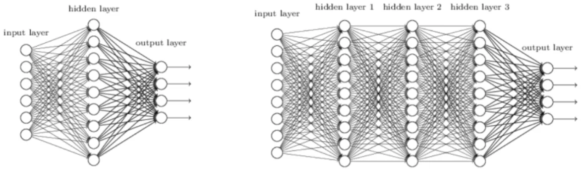
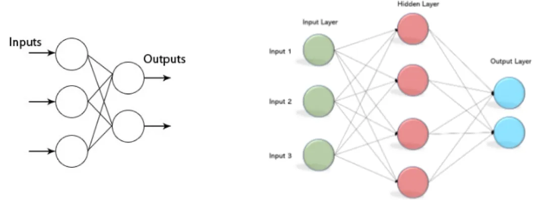
A network is defined as shallow when it only has one hidden layer between the input and output layers; it is considered deep otherwise, as shown in Figure 1.1. This qualification, however, is quite broad as there are no proved evidence about the number that configures either one type or the other. In addition, even though this concept has been investigated for decades, it is still unclear when it is better to use shallow networks instead of deep ones.

According to the Universal Approximation Theorem [7], it is always pos-sible to create a network capable of approximating any complex relation between input and output. In particular, any shallow network with a finite number of neurons in its hidden layer should be enough. However, in the reality, deep networks are more used because they require less resources.

Figure 1.1: An illustrated comparison of a shallow network (left) and a deep network (right). Image taken from [28].

Again, a proof about why this happens is still not available and this belief only follows after a trial-and-error approach on many tasks. In particular, it is believed deep networks may represent a composition of several functions, where previous layers encode simpler features on top of which following lay-ers build more complex ones. For this reason, a neural network can also be defined as a function approximator which tries to model a function between the input and output, but depending on millions of parameters.

The following sections will describe in detail many of the concepts that contribute to define this kind of model and some of its different types.

1.1

Basic Concepts

1.1.1

Neuron

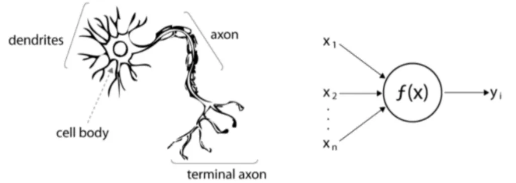
The artificial neuron is the smallest computational unit in a neural net-work; according to the Figure 1.2, it is easily modelled from the biological neuron. All the input signals of a neuron coming from its dendrites are joined with their respective synapse and then, processed by the cell body itself, be-fore being sent to other neurons through the axon.

1.1 Basic Concepts 3

Figure 1.2: The artificial neuron model (right) compared to its biological counterpart (left)1

Even though this could seem quite difficult to be modelled, its mathe-matical translation is very simple: every input signal is represented as a real number, x1, x2, . . . , xn, every synapse with a weight factor w1, w2, . . . , wnand

the output is just the weighted product of all signals. In order to model the firing mechanism of the biological neuron, the so-called bias term b is intro-duced to model a threshold which is associated to every neuron. Given z the output of a neuron, Equation 1.1 shows this mathematical representation.

z = b +X i

wixi (1.1)

After applying some simple algebraic concepts, Equation 1.1 can be rewrit-ten in a more compact way, shown in Equation 1.2, where x is the input vector, w is the weights vector and the summation has been replaced with the dot product.

z = w· x + b (1.2)

1.1.2 Activation Function

The neuron output, as described earlier, is just a linear combination of its input. In the reality, another processing step is employed which consists

of applying a non-linear function f (_{·) to z. It is called the activation}

func-tion and plays an important role in the process of letting a neural network

learn. As a consequence, the updated mathematical representation is shown in Equation 1.3.

y = f (z) = f (w· x + b) (1.3)

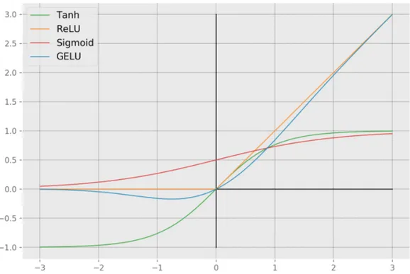
During the decades, many activation functions have been used for mod-elling the learning process of a neural network, in particular the sigmoid function (1.4) and the hyperbolic tangent (1.5). They both have the advan-tage of mapping the input to a fixed range, [0, 1] and [−1, 1] respectively; however, they both suffer of the vanishing gradient problem, which almost prevent large networks to learn at all.

sigmoid(x) = 1

1 + e−x (1.4) tanh(x) =

ex_{− e}−x

ex_{+ e}−x (1.5)

Following the work of Glorot at al. [10] and Krizhevsky at al. [19], a simple activation function such as the Rectified Linear Unit (ReLU) proved to be very beneficial when training particularly large networks and it became the de-facto standard. It is very simple, as shown in Equation 1.6, and avoids the vanishing gradient problem because positive input values very close to 1, linearly approach 1, as it can be see in Figure 1.3. However, it has the

exploding gradient problem, which can almost be considered as the opposite

of the vanishing one. Both problems will be described in Section 1.3.5.

ReLU (x) = max(0, x) (1.6)

Even though ReLU is considered to be the most used activation function nowadays, currently state-of-the-art models, such as the ones described in the following chapters, made Gaussian Error Linear Unit (GELU) [13] popular. It is just a combination of other functions and approximated numbers but

1.1 Basic Concepts 5

the interesting fact is its plot, which is quite similar to ReLU’s one.

GELU (x) = 0.5x(1 + tanh( r 2 π(x + 0.044715x 3 ))) (1.7)

Figure 1.3: Comparison of Sigmoid, Tanh, ReLU and GELU activation func-tions

1.1.3 Main Layers

In the following layer descriptions, a forward pass means the act of feeding an input to the layer and computing the output. More information about this behaviour are described in Section 1.3.

In addition, a feature is every kind of relevant information extracted from data, which is useful to compute the output. As it will be shown, the purpose of many layers is exactly to learn how to extract these features, in order to obtain a feature map.

Fully Connected Layer

The Fully Connected Layer is the simplest type of layers in a neural network. As its name suggests, it has full connections with all the outputs from the previous layer but no connections between neurons in the layer itself. The forward pass of a fully connected layer is just one matrix multiplication with weights, followed by a bias offset and an activation function.

Weights matrix associated to this layer has a shape of (n, m) and a bias vector b, where n is the number of neurons in the current layer (k), while m is the same number but referring to the previous layer (k_{− 1). According to} the Equations 1.1 and 1.3, this operation will compute:

y(k)= f (     w1,1 . . . w1,m ... ... ... wn,1 . . . wn,m         y₁(k−1) ... ym(k−1)     +     b1 ... bn    ) (1.8)

Supposing a simple network with an input layer of shape (2, 1), a fully connected layer of shape (3, 1) and an output layer of shape (1, 1), the result of the fully connected layer is given from the following equation:

y1 = f (     w1,1 w1,2 w2,1 w2,2 w3,1 w3,2     y 0 1 y0₂ ! +     b1 b2 b3    ) =     y₁1 y₂1 y1 3     (1.9) Convolutional Layer

As its name suggests, this layer applies the operation of convolution to its input. In the context of neural networks, however, the definition is slightly different from the pure mathematical one: it is a linear operation that in-volves the multiplication (dot product) of the input and a smaller weights matrix, called filter or kernel. Because of its smaller size, a filter can be

1.1 Basic Concepts 7

thought as a light that slides over the input, applying the convolution on the highlighted portion only. This sliding approach involves just two dimensions, width and height, from left to right, top to bottom. Even though the filter considers two dimensions only, it will extend through all the other dimen-sions, such as depth. In fact, every filter will produce a different feature map which are stacked together along the depth dimension.

This mechanism is governed by some hyperparameters:

• Depth (not to be confused with the dimension): states the number of different kernels to learn that are applied on the same portion of input • Stride: states the amount of neurons/pixel the kernel has to slide from

the previous position

• Zero-Padding: states the number of padding neurons at the borders in order to make the filter fit the input; this will also allow to arbitrarily control output size

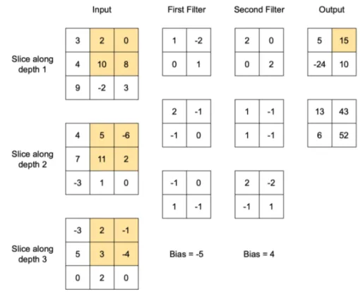
Given an input of size (W i, Hi, Di), a kernel width KW , a stride S, a padding P and the number of kernels to be applied K, the output will be of size (W o, Ho, Do), where Do = K and W o given by the Equation 1.10 (similarly for Ho). An example of a convolution is shown in Figure 1.4: given the input of shape (3, 3, 3), two kernels of shape (2, 2, 3) are applied with S = 1 and P = 0.

W o = W i− KW + 2P

S + 1 (1.10)

Pooling Layer

A Pooling Layer applies a downsampling operation to its input, in order to reduce input dimensionality and the associated number of parameters. Similarly to what happens with convolutional filters, this layer also supposes the usage of a particular filter all over the input; in other words, it applies a function, generally max or average, on portions of input data.

Figure 1.4: Example of convolutional layer output; the highlighted numbers are the ones who contribute to compute 15 in the first output slice, since the first kernel is applied

A pooling operation depends on two hyperparameters: filter width K and stride S. Given an input of shape (W1, H1), the output dimensions are

computed with the Equation 1.11 (similarly for the height). Figure 1.5 shows an example of both max and average pooling with K = 2, S = 2 on an input of shape (4, 4); the colours refer to the portion on which the function has been applied. Note that if the input shape is composed of additional dimensions, such as the depth, this operation will leave them untouched.

This layer with K = 2 is the most common one, together with the

1.2 Types of Neural Networks 9

usually results in information loss.

W2 =

W1− K

S + 1 (1.11)

Figure 1.5: Example of max and average pooling operations

1.2 Types of Neural Networks

Before describing some of the main types of neural networks, layers can be classified based on the position they have in the architecture. For instance, the input layer is the first one which expects model input; the output layer is the last one and is designed according to the task the model has to tackle; and finally, all the others, if present, are called hidden layers.

1.2.1 Feed-Forward Network

A Feed-Forward Network is the simplest type of network where the com-putation flows only from the input layer to the output one and, in particular, iteratively from one layer to the next one. In addition, its structure does not expect back connections or cycles. Strictly speaking, a network of this type is composed of fully connected layers but this term is often used to only state the iterative, one-directional way of computation.

The simplest example is the Single Layer Perceptron network, which is only composed of an input and an output fully connected layers, and its gen-eralization, called Multi Layer Perceptron, because it has at least an hidden layer in between.

Figure 1.6: Single (left) and Multi (right) Layer Perceptron networks2

1.2.2 Convolutional Neural Network

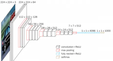
A Convolutional Neural Network is a deep feed-forward network mainly composed by convolutional and pooling layers. They also usually have some final fully connected layers depending the task the model has to address, particularly for classification.

This kind of network is highly inspired to the humans’ visual cortex and the concept of receptive field because smaller portions of data are consid-ered while being processed, as described in Section 1.1.3. Because of their usual architecture and the mathematical operations applied, Convolutional Networks have the following main characteristics:

• They are local connected, as every neuron of a layer is connected to only a local region of its input, as opposed to fully connected layers. As a consequence, number of parameters is highly reduced

• Instead of vectors and matrices, they work with data treated as 3D

volumes (width, height, depth), according to a specific spacial

arrange-ment

• Under the assumption that if a learned feature is useful on a specific spacial position, it will also be useful on another position, filter applied on data slices along the depth dimension can share weights and biases

1.2 Types of Neural Networks 11

• They are translation invariant: if the network learns to detect a par-ticular feature, it will continue to detect it even if it gets translated in another position

Their main and most effective applications involve Computer Vision, with image classification, analysis and recognition, and Natural Language Process-ing, with sentence classification and feature extraction.

Important early works regarding convolutional networks have been pro-posed by Y. LeCun, such as the LeNet [22] architecture. Subsequent famous works are AlexNet [18], GoogLeNet [40] and VGGNet [37].

Figure 1.7: Convolutional Neural Network example: the VGG16 architec-ture3

1.2.3 Recurrent Neural Network

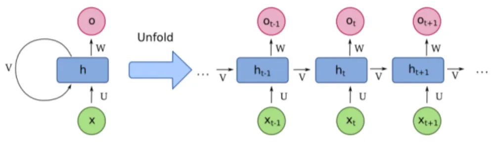
Traditional networks as the ones described earlier suppose every input is independent from the others. Consequently, sequential information are poorly handled. On the contrary, Recurrent Neural Networks perform the same computation on every element of an input sequence, where the output

depends on the previous ones. In particular, they can be viewed as networks with a memory of all that has been computed so far. In order to make this possible, a Recurrent Network can be considered very similar to a Feed-Forward one, with the main difference that the former allows the presence of cycles in its architecture. Actually, this is what characterizes them the most, as shown in Figure 1.8.

Because text and language are inherently sequential, this type of networks became popular for Natural Language Processing tasks, such as, Next Word Prediction or Sequence Labelling.

Figure 1.8: Recurrent Neural Network example; on the right the extended, unfolded version of the network4

For every token in a sequence, it is fed to an hidden layer to compute the related output but the hidden state of the previous token is fed too. By doing so, the predicted output value takes into account also information about previous tokens, just like an informed context.

From an analytical point of view, the equations to compute outputs slightly change, as they have to take into account new and different weights and biases. Generally speaking, given a time step or token position t, the following equations apply:

at= g(U · xt+ V · at−1+ ba) (1.12) 4_{Image taken from https://is.gd/utjo8r}

1.3 How Neural Networks Learn 13

yt= f (W · at+ by) (1.13) W , U and V are learnable weights matrices, ba and by are bias vectors for

computing hidden state activations and outputs, respectively. Such matrices are shared across time steps/token positions so the model will not increase its number of parameters with the size of input.

Because of their structure, Recurrent Networks have the advantage of allowing inputs of an arbitrary dimension; in the reality, however, this poses the problem of long-term dependencies, as it is difficult to keep track of contextual information for rather long sequences. In addition, they are quite expensive to train and slow to compute, due to their sequential nature, and they only get information from the past context instead of the future one too.

Many state-of-the-art models described later in this work focused on tack-ling many of these drawbacks, in order to obtain feasible and powerful lan-guage models.

1.3 How Neural Networks Learn

After modelling a neural network and its architecture, how is it possible to make them learn? How can they really understand their input and decide which answer to return? As it has been said earlier, everything is inspired to the human brain but the reality consists in only learning algorithms which accordingly update numbers.

1.3.1 Hebbian Learning

One of the first learning algorithms has been proposed by D. Hebb in 1949, following the neuroscientific theory often summarized as “cells that

together has the consequence of strengthening the synapse between them, or weakening it otherwise.

From the point of view of artificial neural networks, nodes that tend to be both positive or both negative at the same time have a positive weight connecting them, a negative one otherwise.

In general, this idea does not take into account a ground truth value, so tasks which require a supervised learning approach are not feasible with this learning algorithm.

1.3.2 Gradient Descent

Another learning algorithm is Gradient Descent, which is an instance of local optimization algorithms. On the contrary of Hebbian Learning, this algorithm supposes the knowledge of ground truth values, in order to compare them with the model predicted output. This comparison is made through a

loss function, which has to be continuous and differentiable.

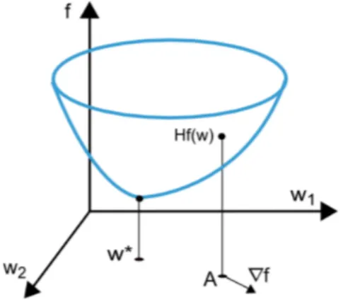
The general idea of gradient descent is to minimize the loss function, by discovering the lowest minimum point of that function, as shown in Figure 1.9. Ideally, when this point is reached, the loss is optimal so model accuracy should be as high as possible.

Figure 1.9: A simple cost function representation; in the reality, more and more parameters are involved5

1.3 How Neural Networks Learn 15

The minimum loss value is iteratively found by computing the gradient of the loss function. Given a N -dimensional space, where N states the number of parameters the model depends upon, the gradient of the loss function with respect to the parameters is a vector whose components are partial derivatives of the loss function. Equation 1.14 shows this formulation, where

L is the selected loss function, y is the expected output value and f (x; θ) is

the predicted output value which depends on model parameters θ.

∇θL(f (x; θ), y) =        ∂ ∂w1L(f (x; θ), y) ∂ ∂w2L(f (x; θ), y) ... ∂ ∂wNL(f (x; θ), y)        (1.14)

After computing the gradient, weights and biases are updated according to the rule in Equation 1.15, where_{∇L is the gradient and η is the learning}

rate. This hyperparameter is particularly important when training neural

networks because it states the magnitude of the gradient updates on the weights. In fact, when this value is too small, the model will train very slowly; when it is too big, the model may not learn as the minimum value could be skipped, resulting in a loss function divergence.

θt+1 = θt− η∇L(f(x; θ), y) (1.15)

1.3.3 Backpropagation

Since the loss function is computed at the end of the neural network, the derivatives shown in the previous section are only valid for the last layer, even though the majority of parameters belongs to intermediate hidden lay-ers. Backpropagation, then, is an algorithm to appropriately compute the gradient taking into account the architecture of the network. In other words,

it propagates the information about the loss back to the input layer by using the concept of computation graph.

Having a mathematical expression, its computation graph is a representa-tion in which the computarepresenta-tion is broken down into separate operarepresenta-tions and each one of them represents a node in the graph. In the forward pass, input values are passed left to right in the graph, computing the operations in the nodes values flow through; in the backward pass, instead, derivatives with respect to the output function are computed.

This kind of differentiation uses the chain rule: supposing a composite function f (x) = g(u(v(x))), its derivative with respect to x is:

∂f ∂x = ∂g ∂u · ∂u ∂v · ∂v ∂x (1.16)

Each partial derivative is calculated along the edges of the graph, right to left, taking into account the operations in the nodes, until the input is reached.

1.3.4

Stochastic Gradient Descent

As the name suggests, this is a modification of the gradient descent al-gorithm which overcomes a drawback: plain gradient descent considers the entire training dataset when computing one update. As anyone can image, this can be very slow or even unfeasible. On the contrary, stochastic gradient descent considers only one sample from the data to update the weight; this sample is chosen randomly among all the dataset. As a consequence, this algorithm is faster but the minimum it usually finds may not be the optimal one because of the variations caused by each sample.

1.3.5

Undesired Effects

Vanishing/Exploding Gradients

Vanishing or exploding gradient is a common problem when dealing with

1.3 How Neural Networks Learn 17

some discoveries in the last few years. This phenomenon happens when gradient-based learning methods and backpropagation are used to train a network, as described in Section 1.3.

Gradients at a specific layer are computed as the multiplication of ents of prior layers, because of the chain rule. For this reason, having gradi-ents in the range (−1, 1) will result in numbers that gets smaller and smaller, until they vanish and will not update the weights. As a consequence, initial layers in the architecture will not receive a meaningful update, resulting in a long training time and considerable performance loss. On the contrary, if weights initialization and gradient computation produce large numbers, exploding gradients will happen, as their multiplication will easily tend to infinity.

Overfitting/Underfitting

Another undesired effect when developing machine learning or statistical models is the overfitting or underfitting of data. The purpose of these models is to find the best approximated function that describes the data. In partic-ular, it should be able to generalize, in order to correctly be applied on new data.

Speaking about overfitting, it can happen under different situations, such as when using a model with too many parameters or when it is trained for too long or when the training data used is not enough. In fact, in such cases, the model will not focus on the relevant relation that describes the data but it will learn also statistical noise and useless information.

Underfitting, on the contrary, can be seen as the opposite problem: it happens when the model can not adequately capture the underlying structure of the data because the representative power is too low or is has been trained for too few time.

1.4 Normalization and Regularization

1.4.1 Dropout

Dropout [38] is a regularization technique used to prevent a model from

overfitting while training. It is different from other techniques, such as L1

and L2 regularization as it does not change the cost function, but instead, it relies on changing the network itself and updating only a subset of weights and biases.

Large neural networks often suffer of co-adaptation: stronger connections between a subset of neurons is learned and they overlook the weaker ones. The direct consequence of this behaviour is that the model will also learn some statistical noise from the training dataset. In other words, it will per-form really well on that dataset but its generalization capabilities will reduce considerably.

Dropout tries to prevent this by randomly deactivating some neurons and their connections with a probability sampled from a Bernoulli distribution of parameter p. As a consequence, only a subset of neurons is trained, breaking the co-adaptation problem and making them more robust because they have to learn features without relying too much on other neurons. After every training iteration, deactivated neurons are restored and a new subset is sam-pled. From a practical perspective, this means that multiple different models are trained at the same time: given the model with n units, it can be thought as a collection of 2n _{smaller networks.}

At test time, no units are deactivated and all weights are multiplied by p to guarantee coherence on the output between both training and test time. In addition, considering all weights together acts as a form of averaging between all smaller models.

A parameter p = 0.5 is quite frequent in the Computer Vision field, even though this technique has been overcome by others, such as Batch Normalization [15]; in NLP, instead, a value p = 0.1 is more common despite difficulties of its application due to the nature of problems.

1.4 Normalization and Regularization 19

Figure 1.10: Dropout intuition; neurons in b) will result in two different models6

1.4.2 Batch Normalization

Because of how neural networks are structured, the output of every layer is passed as input to the following layer and so on, until the output one. This has implications on the distributions of inputs, leading to the concept of Internal Covariate Shift [15], which is the change in the distribution of network activations due to the change in network parameters during training. These shifts can be problematic because the discrepancy between subsequent layer activations can be quite pronounced.

Batch Normalization [15] then, aims to limit the shifting problem by normalizing the output of each layer; in particular, the network will learn γ and β parameters to transform the input distribution in order to have zero mean and unit variance.

Given a mini-batch _{B = x}1,· · · , xm, the first step involves the

compu-tation of mini-batch mean and variance, which are then used to normalize mini-batch values, as shown below.

µ_B = 1 m m X i=1 xi (1.17)

6_{Image taken from https://developers.google.com/machine-learning/} crash-course/embeddings/translating-to-a-lower-dimensional-space

σ_B2 = 1 m m X i=1 (xi− µB)2 (1.18) bxi = xi− µB p σ2 B+ ϵ (1.19) BNγ,β ≡ γbxi+ β (1.20)

Because of its formulation, one of Batch Normalization drawbacks is that it can not be applied to settings where mini-batch size is not big enough to obtain good results, for instance at least 32 or 64. In this case, other forms of normalization are preferred.

1.4.3

Layer Normalization

Layer Normalization [2] has been introduced to address some drawbacks of Batch Normalization, such as the overcomplication needed to apply it in

Recurrent Neural Networks (RNNs) or the requirement of big mini-batches.

Recalling, a mini-batch is a set of multiple examples with the same num-ber of features and it is represented as a matrix/tensor where one axis corre-sponds to the batch and the others to feature dimensions. On the opposite of Batch Normalization, which normalizes over the batch dimension, Layer Normalization learns γ and β parameters (mean and variance) over features, as it is shown in the equations below. As a consequence, these values are independent from other examples, allowing an arbitrary mini-batch size.

µi = 1 m m X i=1 xij (1.21) σ_i2 = 1 m m X i=1 (xij − µi)2 (1.22) bxij = xij − µi p σ2 i + ϵ (1.23)

1.5 Transfer Learning and Fine Tuning 21

LNγ,β ≡ γbxij + β (1.24)

Figure 1.11: Visualization of difference between Batch and Layer Normaliza-tion7

1.5 Transfer Learning and Fine Tuning

Transfer Learning is the process of training a model on a large-scale dataset and then, use the learned knowledge as a base for a downstream task. This type of learning has been quite popular since the ImageNet 2015 Challenge [33], where the winning model showed how powerful such tech-nique could be for Computer Vision. Later on, research in that field literally exploded but other fields, such as NLP, still struggled. In fact, examples of successful transfer learning applied to text were only few and usually too specific to be generalized.

In the last few years, however, pretrained language models showed their power, enabling a generic transfer learning for NLP too. The general pro-cedure, in fact, consists in pretraining a model on a large unlabelled dataset and then, adapting its learned representation on a supervised target task with a new, smaller labelled dataset.

The introduction of BERT [8], whose description will follow in the next chapters, marked huge progress in many state-of-the-art baselines for many

different tasks, such as Question Answering and Sentence Classification. Fol-lowing transfer learning, a fine tuning phase is usually applied: in this case, models are slightly adjusted to improve their performance on a smaller and more specific task. In other words, transfer learning makes a model learn general understanding abilities while fine tuning leverages them to tackle one precise problem.

1.6

Embeddings

From a practical point of view, neural networks expect a numerical input to process when they have to fulfil a task. This kind of input, however, is not composed by random numbers but instead, they semantically represent a high-level concept or object. A simple example is an image, where every number in its encoded representation states the intensity of every base colour for each pixel. Some inputs are intrinsically easy to be represented by num-bers, while other not, such as text. It is not immediate to transform a text in a series of numbers because of all the meanings it conveys, the relations between words, its structure, its similarities and so on.

Vector semantics is a model that tries to encode all these

characteris-tics by taking into account the environment in which every words is usually employed and a vector representation. Such vectors are called embeddings because they embed a word in a particular high-dimensional vector space. Embeddings can be either sparse or dense: the main difference is the dimen-sionality of the vector; the former, in fact, is usually as big as the vocabulary, while the latter has a fixed size, usually about hundreds of values.

Given a vocabulary of size V , an example of sparse embedding is the

one-hot encoding: a vector of size V is associated to every word in the vocabulary.

The encoding for the i-th word will have a 1 in the i-th index and zeros anywhere else. Generally speaking, sparse embeddings can become unfeasible to be used in tasks where the vocabulary size is very big, making dense ones more suitable for them.

1.6 Embeddings 23

Figure 1.12: Example of one-hot encoding of words8

Some other kinds of embeddings follow from the distributional seman-tics research area and the so-called distributional hypothesis, which states that “words occurring in similar contexts tend to have similar meaning”. This hypothesis is the base of many statistical methods for analysing the relations between terms and documents, mainly focusing on counting their occurrences.

1.6.1 Word2Vec

Word2Vec [26] is a set of models designed to compute dense and short word embeddings. The intuition consists of replacing count statistics between words with a binary classifier whose task is to predict whether a word x is likely to show up near another word y.

Given a large corpus of text, Word2Vec will produce a vector space in which word vectors are positioned, according the assumption that word shar-ing a similar context in the corpus will be closely located in the vector space.

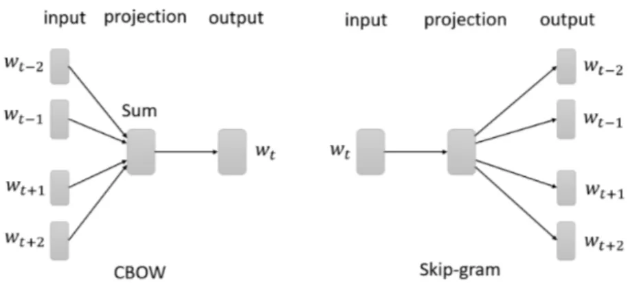
Continuous bag-of-words (CBOW) or Skip-gram are the two models used

by Word2Vec: the former predicts the next word by looking at some sur-rounding context words, while the latter does the opposite, predicting a set of context words given the current word. Once the learning phase for the clas-sifier is done, the embeddings consists of the weights the model has learned

for every word.

Figure 1.13: Word2Vec CBOW and Skip-gram block-diagram example9

Chapter 2

Question Answering

Question Answering (QA) is the field belonging to Natural Language

Processing whose purpose is to create a system which is capable of automat-ically answer questions made by humans using natural language. Every QA system can be classified as closed-domain, when only questions regarding a specific and narrow topic can be asked or when they are limited (i.e. What

is the capital of Italy?), or as open-domain, when basically anything can be

requested (i.e. What was your last travel trip experience like?).

Since the early stages in the 1960s, a knowledge base has been the primary source of information, shifting to information retrieval (IR) approaches in the late 1980s. By definition, a knowledge base is a way of storing complex structured and unstructured data in a form of facts, assumptions and rules; for this reason, this data representation usually requires an expert that has enough knowledge to model it in an appropriate way. Many expert systems, in fact, rely on a knowledge base and an inference model to reason and provide answers. Due to the design, this kind of system is difficult to scale and they are only used for narrow and specific topics.

Nowadays, even though many IR systems are available and used, there is a growing interest in machine reading comprehension (MR) models. Watson [9], from IBM, is an example of QA system based on a huge knowledge base which became famous when it defeated Jeopardy top-player in 2011, putting

the spotlight on how powerful machines can be.

IR and MR models are quite different: the former involve searching for documents, deciding the relevant ones and identifying passages of text that can provide an answer, while the latter assume a question and a passage will be given and their purpose is to understand them, in order to look for the correct answer.

2.1

Evaluation Metrics

After developing a system, it has to be evaluated according to some met-rics; their choice usually depends on the particular task and data format the model returns, in order to obtain real and meaningful information. In other words, the purpose of evaluation is answering the question how well does the

system work?. Regardless task type, either it is generic such as classifica-tion or regression, or more specific, the main idea is always to compare the

predicted output from the model and the ground truth, representing the real expected values.

Confusion Matrix

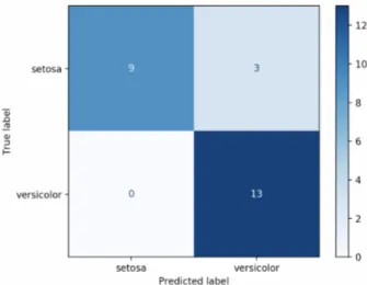
Before digging into some of the main metrics, it is important to under-stand the Confusion Matrix, which is a tabular or visual representation of the relations between predicted labels and real ones from the ground truth, of size (num labels, num labels). Figure 2.1 shows the confusion matrix on a subset of the Iris Dataset [1], restricted to two classes only.

This representation is particularly useful because it allows to obtain the required information to compute multiple metrics:

• True Positive (TP): number of correctly predicted examples of the positive class

• False Positive (FP): number of examples whose predicted class is the positive one but the actual one was another

2.1 Evaluation Metrics 27

Figure 2.1: Confusion Matrix computed on a subset of the Iris Dataset

• False Negative (FN): number of examples whose actual class is the positive one but another one was predicted

• True Negative (TN): number of correctly predicted examples of all the other classes

Accuracy

Accuracy is one of the simplest metrics as it states the ratio between correctly predicted values and total number of predictions.

Accuracy = T P + T N

T P + T N + F P + F N =

# correct predictions

# total predictions (2.1)

Precision

Precision is a classification measure that intuitively states the ability of a classifier not to label as positive samples that are negative; it is also called

Positive Predictive Value (PPV). This metric can be more meaningful than

accuracy when classes in a dataset are imbalanced: in fact, in that case the model would correctly predict the most frequent class, thus resulting in a high accuracy rate; in the reality, however, it may not be learning at all the

least frequent classes.

P recision = T P

T P + F P (2.2)

Recall

Recall intuitively states the ability of a classifier to find all the positive examples; it is also called Sensitivity. If used alone, it may not be very meaningful, as it is easy to obtain the maximum recall; to avoid this scenario, it may be necessary to compute also statistics about non-relevant examples, such as precision.

Recall = T P

T P + F N (2.3)

F1 Score

The F1 Score, or F-measure, is the harmonic mean between precision and recall. In case of binary classification, it can be seen as a measure of a test’s accuracy. It is mainly used in settings where both precision and recall are important, such as in Natural Language Processing.

F1 = 2·

P recision· Recall

P recision + Recall (2.4)

Generally speaking, the Fβ score is given by the Equation 2.5, where β states how many times recall is more important than precision; for this

reason, the F1 gives the same importance to them.

Fβ = (1 + β2)·

P recision· Recall

(β2· P recision) + Recall (2.5) Exact Match

In Natural Language Processing, Exact Match (EM) score is a simple but very useful metric which states the ratio between correctly predicted values and total number of predictions, with the constraint that the predicted value must be exactly the same as the expected one.

2.2 Datasets 29

Considering the example in Figure 2.1, we treat the “versicolor” class as the positive one, obtaining the following metrics:

T P = 13 F P = 3 F N = 0 T N = 9 Accuracy = T P + T N T P + T N + F P + F N = 13 + 9 13 + 9 + 0 + 3 = 0.88 = 88% P recision = T P T P + F P = 13 13 + 3 = 0.8125 = 81.25% Recall = T P T P + F N = 13 13 + 0 = 1.0 = 100% F1 = 2· P recision· Recall P recision + Recall = 2· 0.8125· 1.0 0.8125 + 1.0 = 0.8965 = 89.65%

2.2 Datasets

Many dissimilar dataset are available, such as TriviaQA [16], WikiQA [45], WikiReading [14], MSMarco [4] and SQuAD [30], with diversities on the way questions and answers have been created, the number of questions and the source documents considered. For instance, WikiQA is very sim-ilar to SQuAD, as it also considers Wikipedia documents but its purpose is sentence selection instead of span extraction. Some of them also assume presence of questions whose answers are not in the related text passage; the intuition behind this choice is that models should also be able to evaluate when information provided are enough to return a meaningful answer, oth-erwise it is better to avoid answering. However, due to every dataset key aspects, not all machine reading question answering datasets can be used for the span extraction task; in this work, we mainly focused on the SQuAD one.

2.2.1

SQuAD Dataset

Stanford Question Answering Dataset (SQuAD) is one of the biggest

read-ing comprehension dataset that is available to the community. In fact, it is a collection of more than 100000 question-answer pairs, created by crowd-workers on a set of 400+ Wikipedia articles. In particular, answers have been annotated manually by selecting a span of text in the passage, together with the starting index. For this reason, this dataset can be used with every model capable of span extraction.

Figure 2.2: Example of paragraph from SQuAD v2.0 dataset, with questions and answers

One thing characterizing SQuAD v1.1 [31] is the assumption that ev-ery question has at least an answer in the provided text; in other words, a model trained on it will always predict an answer, even though it is not relevant. This assumption, of course, oversimplifies the reality as situations of uncertainty and lack of information could arise in every moment.

Consequently, SQuAD v2.0 [30] has been released as a brand-new dataset during 2018. The inclusion of about 40000 new pairs of unanswerable ques-tions is supposed to tackle the assumption described earlier and these new information are marked by the attribute is_impossible set to True.

The train dataset, however, is not balanced with respect to the question type: as you can see from the summarizing table below, the ratio is 67%-33% in favour of answerable questions. Instead, the dev dataset is well balanced. In addition to train and dev, an evaluation script on the dev set has been provided, allowing researchers to evaluate their models before submitting results to the official leaderboard [39]; this is necessary because the real

2.2 Datasets 31

Train Dataset Dev Dataset

Questions Unanswerable Questions Unanswerable SQuAD v1.1 87599 – 10570 –

SQuAD v2.0 130319 43498 11873 5945 Table 2.1: Questions distribution by type across datasets.

figures appearing online are evaluated on a test set that has been kept closed-source. According to the scores shown online, SQuAD v1.1 is considered solved as many models exceeded the human performance of 82.304 EM and 91.221 F1 measure. Version 2.0, instead, is more challenging (86.831 EM and 89.452 F1 measure) and new models are being developed week after week.

The dataset is released as a JSON object, whose every inner object rep-resents a specific topic; each one of them is a collection of one or more text paragraphs with the associated question objects and answers, when available. An example of SQuAD v2.0 object about Normans, with both an impossible and a possible questions can be seen in Appendix B.1.

Results Comparison

Following the brief introduction about the dataset, Table 2.2 shows a comparison between current state-of-the-art models and previous approaches tackling this problem. In particular, some of them will be described in detail in the following chapters, in order to understand breakthrough changes which led to performance improvements.

Question answering approaches to this dataset changed a lot during the decade; chronologically, in fact, the following systems have been implemented to address this task:

• Sliding Window Approach [32] (2013): baseline system involving the usage of lexical features; bag of words are created taking into account both the question and the hypothesized answer

• Logistic Regression model [31] (2016): extracts several types of fea-ture for every possible answer, most of which are lexical ones, such as matching word and bigram frequencies and lexical variations; they all contribute to make the model pick the right sentence

• BiDAF [35] (2016): this model leverages many different “blocks”, such as CNNs, LSTMs and attention mechanisms, focusing on both con-text and question information in a bidirectional way. It will compute probabilities for every token to be the start and the end of the answer span

Model SQuAD v1.1 SQuAD v2.0

F1 EM F1 EM Human Performance * 91.2 82.3 89.45 86.8 Sliding Window 20.2 13.2 - -Logistic Regressor 51.0 40.0 - -BiDAF (single) 77.3 67.7 - -BERTBASE 88.5 80.8 - -BERTLARGE 90.9 84.1 81.9 78.7 RoBERT a 94.6 88.9 89.4 86.5

Table 2.2: Performance comparison of state-of-the-art models on both SQuAD v1.1 and v2.0 dev datasets. * as stated in [31], [30].

2.2.2

OLP

In addition to SQuAD, another dataset has been used to experiment with the investigated models: it is the OLP dataset [6] [5] developed by a workgroup at Bielefeld University. As it is still under development, it is not publicly available yet. As opposed to SQuAD, OLP is a Question Answering dataset that focuses on free text and knowledge base integration.

One of the main differences between SQuAD and OLP is the fact that the latter is composed of closed-domain questions; in particular, it is about

after-2.2 Datasets 33

game comments of football matches. For this reason, many questions required some degree of knowledge and semantic processing, as the real answer was not explicitly stated in the text.

In the next sections, there will be a description of the work done to preprocess, normalize and convert OLP to a SQuAD-like format, in order to feed them to our Question Answering models.

2.2.3 Preprocessing

As it can been seen from Figures 2.3, 2.4, 2.5, the structure is very differ-ent, as it is composed of three kind of CSV files: Question, Annotation and Tokens.

Given a specific topic, the first file contains a list of all the questions about that article, with information such as the ID and the correct answer got from a Knowledge Base; the Tokens file, instead, contains the entire text passage, token by token, with specific offsets (character-based, token-based and sentence-based); finally, the Annotation file contains all the information about the hand-made annotations on the text. This file can be considered the way of linking together questions and texts, as both IDs, offsets and answers are stated.

With support from Simone Preite and Frank Grimm, we tried to deeply understand how the dataset was composed and to which extent it was dif-ferent from SQuAD, in order to write the appropriate logic to do a con-version. We wrote many Python scripts to automatically normalize and build the dataset in the proper format but we also had to manually fix mismatches between annotations and questions or wrong knowledge base an-swers. In addition, we removed duplicate entries and cleaned offsets values, as multiple whitespaces caused them to be unreliable. In addition, we added is_impossible information to every question by checking whether the an-swer was explicitly stated in the text or not.

Figure 2.3: Example of questions file from OLP dataset

Figure 2.4: Example of tokens file from OLP dataset

2.2.4

Conversion

After preprocessing OLP, the next step was its conversion: we wrote another Python script to automatically generate the JSON file with the SQuAD-like format, starting from the new data. Unfortunately, we had to take into account maximum sequence length of text paragraphs: OLP texts, in fact, were usually longer than the ones in SQuAD, as shown in Table 2.3, or the ones used for pre-train the models. While converting the dataset, then, we added an option to automatically split long paragraphs into shorter ones belonging to the same topic. This operation, however, involved also a careful handling of questions and annotations, in order to avoid dan-gling references. For instance, splitting took into account entire sentences, avoiding cut phrases between paragraphs and questions about the same topic

2.2 Datasets 35

Figure 2.5: Example of annotations file from OLP dataset

Tokens Per Paragraph 0-999 1000-1999 2000-2999 3000-3999 >4000

Number of Paragraphs 101 26 4 1 1

Table 2.3: Distribution of OLP paragraphs by number of tokens

were replicated in every resulting paragraph. We finally wrote also the ap-propriate logic to split the resulting dataset into a train and dev splits, so that it can be used to fine-tune a Question Answering model, defaulting to a 70%-30% split.

Chapter 3

Transformers

In this chapter there will be a discussion about the Transformer Archi-tecture [41] and its benefits, making it the basic building block of almost all the current state-of-the-art models available.

Seq2seq is one of the most frequent tasks in NLP; in fact, as its name suggests, it involves sequences processing. The main examples are the trans-lation of a sentence between two different languages or the summarization of a long text. They used to be addressed through Recurrent Neural Networks (RNNs): two networks of this type were stacked one after the other; the first one acted as an encoder while the following one as a decoder. The encoder part in only used to obtain a hidden state representation of the input, called

context vector which is then fed to the decoder, that used it as additional

information to predict target tokens.

Unfortunately, the longer the sequence, the more difficult it was to en-code the meaning in a fixed-size vector. In addition, this model is sequential by definition, as each state needs the previous one as input; for this reason, its training can’t take advantage of parallel computation, resulting in long training time, often without the expected results. On the other side, a Trans-former can execute everything in a parallel fashion because of its design and its Attention mechanism let it process the entire sequence at once, in order to get a better representation of the relationships between tokens.

3.1 Input

Text sequences are fed as input to the model through their embedding representation. In this case, their size is dinput = 512 but this is just an hyperparameter that can be set, as it indicates the longest representable

sequence. In particular, a vector of that size will be created for every token appearing in the sentence. Then, assuming a sequence of T tokens, input will be a matrix of size T × dinput. Every sentence will be processed as a sort

of set of token: this, however, has the drawback of losing information about their order.

3.1.1

Positional Embeddings

Given the parallel nature of this architecture, the model needs a way to encode tokens ordering of the given sentence. The intuition here is that a particular pattern can be instilled in the embeddings: for each token, a positional embedding conforming to that pattern is added to the normal one. Following that, the model will be able to learn the pattern and rebuild the original word ordering.

In this case, the addition is given by a sinusoidal signal with different frequencies and phases based on position (sin for even positions and cos for odd ones), but this is not the only possible choice: one benefit of the chosen one is the ability of scaling well with sequences of different length. In particular, given a token at position j in the sentence, every element i of its positional embedding vector is defined as:

P E(i, j) =    sin(wk· j), if i = 2k cos(wk· j), if i = 2k + 1 with wk= 1 10000demb2k (3.1)

The resulting positional embedding vector will be:

⃗ pe_j =

h

sin(w1· j) cos(w1· j) · · · sin(wdemb

2 · j) cos(w

demb

2 · j)

i

3.2 Architecture 39

3.2 Architecture

A Transformer can be just considered as a collection of blocks where information flow through; a visual representation is shown in Figure 3.1. The two main parts are the Encoder stack (left side in the image) and the

Decoder stack (right side in the image). Both stacks have the same number

of layers, which are N = 6; the data is fed to the first encoder, processed by the entire Encoder stack and the passed to the Decoder stack which returns the output representation. Ideally, it is a simple, sequential architecture but, as it will be described in the following sections, the reality is quite different, with many parallelized computations. This is due to the fact that each token can flow through the architecture almost independently from the other ones. Furthermore, every encoder in the stack do not share its learned weights with the other encoders.

Figure 3.1: Encoder-Decoder representation of a Transformer model archi-tecture1

Finally, on top of the architecture there are a Fully Connected layer to-gether with a Softmax one, so that the output from the Decoder stack can be converted into a logits vector, where each value refers to a word in the vocabulary. The Softmax transforms this vector in a probability distribution from which the next token can be predicted.

3.2.1 Encoder

Every Encoder is a stack of three types of layers: Self-Attention,

Feed-Forward Network and Add & Normalization, with skip connections.

Self-Attention layer is the most important mechanism that makes a Transformer a powerful model and it will be described in detail in the next section.

The Feed-Forward Network is basically a stack of two Fully Connected layers with a ReLU [27] activation function in between. Assuming input is of size dinput = demb= 512, the first layer will project it to a dimension 4 times

bigger, having a inner size of dinner = 2048; the second layer, instead, will

output it back to the original size. Given Wi, bi, i∈ {1, 2} the weights and

biases of the the layers and x the normalized attention scores, this network will apply the following transformation:

F F N Layer(x) = max(0, xW1 + b1)W2+ b2 (3.3)

Both the Feed-Forward Network and the Self-Attention Layer have a skip connection around them: the purpose of the Add & Norm Layer is to sum the processed output from the previous layer with the same, unprocessed input got from the residual connection, and then, to apply a LayerN ormalization [2] on the resulting data, in order to normalize across features and indepen-dently from examples. As it has been shown in [12], skip connections are useful for mitigating the vanishing/exploding gradient problem, letting huge deep neural networks to be successfully trained.

1_{Image taken from [41]}

3.2 Architecture 41

Figure 3.2: Encoder block of Transformer architecture2

3.2.2 Decoder

The Decoder is conceptually very similar to the Encoder counterpart: it takes a shifted masked embedding as input together with the Encoder stack output. The latter is given to every Decoder in the stack while the former only to the first one. During the decoding phase, it does not make sense to know words after the current one: for this reason, the embeddings gets shifted and masked with zeros in order to let the model focus on only the previous tokens. This new information is then used by the Attention mechanism to incorporate it with contextual data for the whole sentence, given by the Encoder stack. Finally, the Feed-Forward Network and the Layer Normalization will apply the same transformations as described earlier.

Figure 3.3: Decoder block of Transformer architecture3