Modelling of the sedimentation phenomenon of solid particles immersed in a turbulent fluid

(1)

SCUOLA DI INGEGNERIA E ARCHITETTURA

DIPARTIMENTO di INGEGNERIA CIVILE, CHIMICA, AMBIENTALE E DEI MATERIALI DICAM

CORSO DI LAUREA MAGISTRALE in INGEGNERIA CHIMICA E DI PROCESSO

TESI DI LAUREA MAGISTRALE in

Dinamica e Controllo dei Processi Chimici

M

ODELLING OF THE

S

EDIMENTATION

P

HENOMENON OF

S

OLID

P

ARTICLES

I

MMERSED IN A

T

URBULENT

F

LUID

CANDIDATO: RELATORE:

Salvatore Evola Chiar.mo Prof. Alessandro Paglianti

CORRELATORI:

Prof. Giuseppina Montante Dr. Claudio Pereira Da Fonte

Anno Accademico 2018/2019 Sessione III

(2)

(3)

3

Abstract

Settling phenomenon of solid particles immersed in a turbulent fluid has been investigated, in a condition of free-stream turbulence.

Since structures formed onto this condition are complex, it is difficult to predict exactly how particles move. It is thus appropriate to conduct deepen studies of the phenomenon and carry out simulations to describe particles’ settling velocity.

In order to define a new correlation for the evaluation of particles’ settling velocity, different literature correlations and parameters have been exploited.

Langevin dynamics has been used to describe fluid’s motion, and by considering several forces acting on particles (buoyancy, drag, gravitational and virtual mass), it has been possible to evaluate their settling velocity, through a computational approach. Data have been obtained by varying characteristic properties, such as kinetic energy, its rate of dissipation, and physical properties of fluid and particles.

Aiming to find a reliable correlation which best explains the settling phenomenon, results in output from simulations have been compared with that deriving from proposed correlation. Encouraging results have been obtained over the range of operating conditions examined.

(4)

4

Introduction

The modelling of sedimentation, suspension and fluidisation phenomenon of solid particles immersed in a turbulent fluid is of considerable importance for the chemical industry and environmental studies.

Settling behaviour of particles in turbulence flow can be found in various natural processes, such as suspended particles in the atmosphere, sedimentation in rivers and turbidity currents on the coast. It also occurs in much industrial equipment of, among others, pharmaceutical, food industry, chemical and biochemical reactor.

In the civil context, the study of dispersion and deposit of solid particles is used in designing some branches in sanitary systems useful for the treatment of drinking and purification water. While, common applications in environmental engineering aim to characterize the dispersion of particles, both in the atmosphere and in water bodies.

One more example of solid particles dispersion and sedimentation in the environmental field is linked to the disaster that recently occurred in the forests of Australia, where 25.5 million acres have burned, thus pouring numerous solid particles into the atmosphere through the wind. This is an effective example of solid particles immersed in a turbulent fluid, that allows comprising the extremely importance of correct prediction of particles motion.

The studying of settling phenomenon is widespread in chemical engineering; for this reason, it is a useful tool for investigating particles behaviour flowing into equipment applied in unit operations.

Types of equipment involve solid particles, in granules, used as raw materials and/or industrial solutions. Typical examples of applications in chemical industry may be the catalytic fluidized bed cracking present in the refinery, sedimentation tanks and crystallises for the separation of suspensions, fluid beds used as reactors to promote contact between phases, more generally in all processes with solid catalysts.

Since particles trajectory is influenced by turbulence flow, it is difficult to predict their exact path. Those random motion inspired many authors to conduct studies in this regard.

(7)

7

Turbulence was investigated experimentally since the end of the nineteenth century, thanks to Reynolds' researches. His experiment demonstrated the fundamental difference between the laminar and turbulent flow. Reynolds observed how the motion of the fluid was related to a dimensionless parameter, later to be known by its own name.

In 1921 the English physicist G.I. Taylor proposed the concept of homogeneous and isotropic turbulence, valid only in the free space, which represents an ideal case of turbulent flow in which the dynamics of fluid motion is neither influenced by interactions with tank walls nor by any average velocity field.

This concept has proved effective in the study of small turbulence scales, despite real turbulent flows are not homogeneous and isotropic.

The turbulent flow, due to the mixing of the fluid particles, is characterized by a high diffusivity and levels of vorticity. The structures that are formed in this regime are defined vortices (or eddies), and these tend to join and separate, to rotate and stretch.

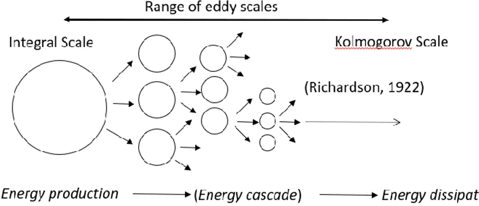
L. Richardson in 1922 supposed the phenomenon of the cascade of energy, in which there are structures of different sizes, whereby non-linear interactions energy is transferred from the largest vortices to the gradually smaller ones, until the energy is dissipated by the effect of viscosity, as heat.

Kolmogorov in 1941 honed the idea of L. Richardson giving it a quantitative form. He supposed that the cascade transfer takes place through an energy flow that defines the average rate of dissipated kinetic energy.

The knowledge of turbulent flow and settling velocity of particles involves the study of forces acting on particles. It is important to underline that, referring to free-stream turbulence, drag coefficient contained into the equation of drag force doesn’t have a clear mathematical expression.

For this reason, several experimental and computational studies were done to characterise the dynamics of particles in mechanically generated free-stream turbulence. However, there is still no universally accepted methodology that considers how random fluctuations of fluid phase influences solid particles.

(8)

8

Improving the fundamental knowledge of particle dynamics in turbulent flows is of considerable importance, for mainly, for the development of robust computational models for the design, optimisation and control of suspension and sedimentation processes.

This study proposes to analyse dynamics’ particles in turbulent flow from a computational point of view and it has been developed thanks to a collaboration with the University of Manchester (UK).

An overview of main studies on the subject carried out by Spelt and Biesheuvel, Lane et al., Brucato et al. and Magelli et al. are presented in Chapter 1.

According to the current knowledge of the phenomenon, motivation and objectives of this study are explained in Chapter 2.

The underlying methodology of this project, described in Chapter 3, illustrates the principles used to carry out simulations and obtain experimental data.

In Chapter 4, a numerical model has been developed to simulate the trajectory of inertial particles in modelled turbulence, using Langevin dynamics, in § (3.2).

A sensitive analysis has been made under different conditions, in order to verify the assumptions, described in Chapter 3, and to obtain the most suitable conditions for the computational environment.

After this analysis, numerical simulations have been conducted to produce a data set of settling velocity.

A new correlation, based on analysed principles and results obtained, has been proposed to explain the settling velocity of solid particles in turbulent flows.

Eventually, project conclusions are presented in Chapter 5, while future works and exploitation purpose are illustrated in Chapter 6.

(9)

9

Chapter I

− State of Art

1.1 Background

Since many types of equipment involved in process industry work with solid-fluid mixtures, understanding of how those two phases interact is of fundamental importance.

When a particle falls in a still fluid it is subject to a force called Drag Force (𝐹_𝐷), which acts in the direction of motion. Drag Force is a function of different factors, that for fluid at rest is expressed by the following relationship:

𝐹_𝐷 =1 2𝜌𝑓 𝑢𝑡

2_𝐶

𝐷 𝐴𝑝 _(1.1)

where 𝜌_𝑓 is the fluid density, 𝐴_𝑝 is the area projected by the particle on a plane normal to the relative velocity 𝑢𝑡, and 𝐶𝐷 is the Drag coefficient which is a dimensionless number that

is determined experimentally.

When the fluid phase is at rest, or in laminar motion, a great deal of experimental information is available for many-particle shapes and physical situation, whether or not the relative motion between the two is able to induce turbulence in the fluid phase in the proximity of the particle. In such cases, a reliable estimate of the relevant 𝐶𝐷 can be easily obtained [16].

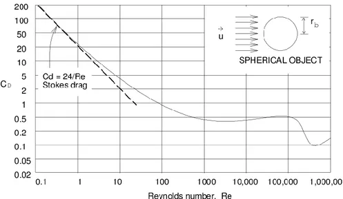
An example of the relationship between the particles’ Reynolds number (𝑅𝑒_𝑝) and the experimental drag coefficients of spheres is shown in Fig. 1.

(10)

10

Fig. 1 – Plot of drag coefficient 𝐶𝐷 against particles’ Reynolds number for the fluid at rest.

In this case, the particle drag coefficient 𝐶𝐷 depends only on the particles’ Reynolds number:

𝑅𝑒𝑝 =

𝜌 𝑢_𝑡𝑑_𝑝

𝜇 (1.2)

where 𝜌, 𝑑_𝑝, 𝜇 are density, diameter and viscosity’ particle, respectively.

With reference to a spherical particle, the continuity and momentum balance equation can be analytically solved leading to the well-known Stokes law, which can be put in the form [14]:

𝐶_𝐷 = 24

𝑅𝑒_𝑝 (1.3)

That is not valid for higher Reynolds number, and drag coefficient referring to spherical shapes of the particle is correlated on a heuristic basis.

At Reynolds numbers around 1000, the drag coefficient begins to level off and stays approximately constant. This range is known as Newton region.

𝐶_𝐷 = 0.44 (1.4)

When the Reynolds number increases between 105 and 106, the drag coefficient rapidly decreases and then increases again, due to the changing of boundary layer region which modifies the pressure distribution around the particle.

(11)

11

Solid particle falls in still fluid by means of the gravitational field, and it undergoes to three forces, like gravity, hydrostatic and drag. After a transient field, velocity becomes steady and the force balance can be written as:

𝐶_𝐷𝜋𝑑𝑝 2 4 1 2𝜌𝑢𝑡 2 ₌𝜋𝑑𝑝 3 4 (𝜌𝑠− 𝜌) (1.2)

Where u_t is the terminal velocity, and it can be obtained from

𝑢𝑡= (

4𝑔𝑑𝑝 (𝜌𝑠− 𝜌)

3 𝜌 𝐶_𝐷 )

1/2

(1.3)

However, many situations involving free-stream turbulence, which can be generated by various sources. In this case, the particle drag coefficient 𝐶𝐷 could be widely different with

respect to the case of fluid at rest.

Free-stream turbulence refers to a system, like stirred reactors, where the presence of non-organised structures, as eddies, influences unpredictably fluid motion, therefore particles motion is complex to study.

Unfortunately, relative few data are available on the effect of free-stream turbulence on particle drag coefficients, especially for the particle sizes typically involved in the equipment of process industry [14].

Several studies on the calculation of drag coefficient have been addressed over the years, and they have briefly reported through the next paragraphs.

Most of them considered the hypothesis of homogeneous isotropic turbulence introduced by Taylor, thus they demonstrated that the settling velocity of heavy particles is enhanced by turbulence, due to the preferential sweeping phenomenon of particles along pathways between vortices.

The fluid dynamics of multiphase stirred equipment is complex, and the effective particle settling velocity in diluted suspension was shown to be smaller than that in a still liquid [2]. Bec et al. investigated the effect of gravity stemming from the density difference between particles and fluids on the settling velocity and clustering behaviour of particles in turbulence, by Direct Numerical Simulation (DNS). This study confirmed the acceleration (1.5)

(1.6) Eq.(1.6).

(12)

12

effect of particle inertia on the settling velocity and showed that the effect depends on the Stokes number and the Froude number [1].

Yang and Lei studied the behaviour of preferential sweeping in the low vorticity region, condition of homogeneous isotropic turbulent flows. They pointed out that preferential sweeping is controlled by small scales, as stated by Kolmogorov’ hypothesis (reported in §1.4), but large turbulent scales also affect the increasing movement of the settling particles. This study showed that the flow vorticity is minimized when the Stokes number is close to one, which corresponds to the maximum increase in the settling velocity [11].

Zhou and Cheng studied the falling in the turbulence of a single large-sized particle of a density slightly heavier than water. They found that the settling velocity cannot be related to turbulence intensity or to the Stokes number. However, the drag coefficient of particles coming out from their experiments is significantly larger than the standard values; this might lead to a decrease in settling velocity. The small particle density differences from the carrier fluid might also play an important role in this reduction [4].

Magelli et al. [12] and Brucato et. al [3] have carried out studies taking into account the parameter 𝑑_𝑝/𝜆. Brucato et al. obtained a direct measurement to calculate the drag coefficient, while Magelli et al. evaluated an average settling velocity by fitting the model predictions to experimental data.

Spelt and Biesheuvel proposed an analysis using a dimensionless parameter 𝛽, that is the ratio between the turbulence intensity and the rise velocity of the bubbles in still fluid. After studying the phenomenon for bubbles, they extended those case to that of particles, showing how the 𝛽 value affects the settling rate of them [2].

Lane et al. [7] initially proposed a correlation involving Stokes number to explain turbulence effects on drag coefficient, by using available literature data. After some years, they noticed that the phenomenon is better explained also with the Richardson number.

This study is based on the analysis conducted by Spelt and Biesheuvel (1997), Brucato et al. (1998), Lane et al. (2007), Magelli et al. (2008), that investigated the behaviour of solid particles immersed in a fluid in free-stream turbulence.

(13)

13

1.2 Previous studies conducted

1.2.1 Spelt and Biesheuvel (1997)

Spelt and Biesheuvel initially presented results of approximate analyses and numerical simulations of gas bubbles motion. After that, they adapted their previous study to that one related to solid particles motion, considering high Reynolds number under the hypothesis of homogeneous isotropic turbulence.

In order to simulate turbulent self-diffusion, settling and dispersion of small rigid particles, studies were conducted involving many Fourier modes varying randomly in space and time. The forces exerted by the surrounding fluid on a settling particle are described by supposing that it acts on a rigid sphere in an inviscid unsteady non-uniform rotational flow (Auton, Hunt & Prud'homme 1988). This drag force lead particle to settling steadily at high values of Reynolds number in still fluid; a good approximation for drag force can be obtained by calculation based on viscous potential flow theory (Moore 1963).

In these conditions, the dominant contribution to the statistics of the particle motion is associated to the autocorrelation function, with considering low-intensity turbulence and characteristics length scales of the same order of magnitude as those used for velocity relaxation of the particles.

They have found a satisfactory agreement between the analyses and the simulations, with a small value of the ratio between the turbulence intensity (𝑢₀) and the settling velocity of the particles in still fluid, 𝛽 (Eq. (1.9)).

For larger values of 𝛽 it is conceivable that the instantaneous small-scale vorticity structure will become more important for statistics’ particle motion, where it is governed by acceleration reaction forces.

Spelt and Biesheuvel used the Eq.(1.7) proposed by Thomas et al. (1984), that combines the expression of motion of small particles immersed in liquid, subjected to forces acting in an unsteady inviscid rotational flow, with that one typical of the drag force.

(14)

14 𝑑𝑉 𝑑𝑡 = 3 𝐷𝑈 𝐷𝑡 − (𝑉 − 𝑈) × 𝛺 − 2𝑔 − 1 𝜏_𝑏(𝑉 − 𝑈) (1.7)

Where 𝑉 is the particle’s velocity, 𝑈 is the fluid velocity, determined by Direct Numerical Simulations (DNS). Ω = ∇ × 𝑈 is the vorticity, while time constant 𝜏_𝑏 is:

𝜏_𝑏= 𝑎

2

18𝜈= 𝑉𝑇

2𝑔 (1.8)

where 𝑎 denoting the equivalent particles radius.

Various dimensionless parameters were used to characterise the motion of the particles. 𝛽 =𝑢0 𝑉_𝑇 (1.9) 𝜇∗ ₌ 𝐿11 𝜏_𝑏𝑉_𝑇 (1.10) 𝜆∗ = 𝜆 𝜏_𝑏𝑉_𝑇 (1.11)

𝜇∗ relates the relaxation time 𝜏_𝑏 of the particle to the characteristic time scales of turbulence. The integral length scale 𝐿11 is a measure of the size of eddies in the flow, and thus of the

spatial variation of the turbulence.

𝜆∗_{relates the Kolmogorov scale of dissipative eddies (𝜆), with the integral time scale 𝑇} 𝐿,

which is a measure of time variation of turbulence, and with relaxation time 𝜏_𝑏.

They used a grid turbulence 𝑇𝐿/(𝐿11/𝑢0) approximately constant, without considering

𝑇_𝐿/𝜏_𝑏 as an independent group*. It was specifically examined the case in which turbulent intensity is less than the particle settling velocity, i.e. 𝛽 ≪ 1. An increasing of 𝛽 leads to an increase in settling velocity, thus particles drift easily through eddies. The group considered, 𝜆∗, was used to compared different energy spectrum functions, as showed in Fig. 2.

By varying 𝛽, through variation of 𝑢₀, changes in turbulence’ structure were studied, with fixed values of 𝜇∗_{, 𝜆}∗_{, or both.}

(15)

15

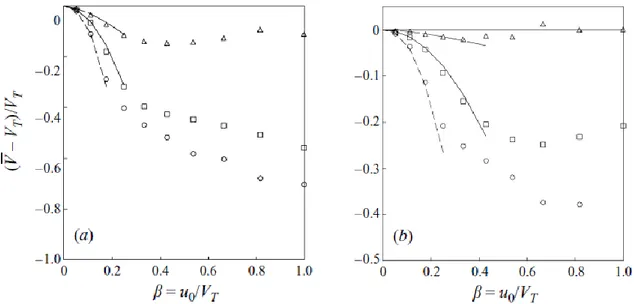
Fig. 2 – The difference between the mean velocity of the rise of a particle 𝑉̅ in isotropic turbulence and its

value in still fluid 𝑉𝑇, as a function of 𝛽. (a) □,⸺, Kraichnan spectrum with λ* = 1 and 𝜇 ∗= (𝜋/2)1/2; ∆,⸺

⸺, von Karman-Pao spectrum with fixed Taylor microscale (λ* = 1); ○,- - - -, von Karman-Pao spectrum with fixed integral scale (𝜇 ∗= (𝜋/2)1/2_{). (b) As in (a) but with λ* = 4 and}_{𝜇 = 2(2𝜋)}1/2_{Curves show the}

analytical results for small 𝛽. [9]

A higher value of the dimensionless group 𝑇𝐿/𝜏𝑏 indicates whether the particles quickly

respond to the turbulent velocity fluctuations.

In order to determinate correlation functions, fixed values for particles velocity and other parameters were considered. Simulations were carried out by involving a single particle released with a certain value of 𝑉𝑇, valid for a still fluid, with its trajectory calculated by a

fourth-order version of the Bulirsch-Stoer scheme (Press et al. 1991) over a sufficiently long time, typically equal to 𝐿₁₁= 𝑢₀.

Referring to the case of free-stream turbulence, that takes place when 𝛽 increases its value from 0 to 1, the deviation of mean settling velocity 𝑉_𝑆, from its value in still fluid decreases up to 50%, due to an increase of turbulence intensity.

Therefore, from Fig. 2, it is possible to conclude that mean particle velocity gets lower with increasing turbulence intensity, in the range of 𝛽 = 0.3 ÷ 0.5. For higher values of turbulence intensity, the particle velocity increases again or becomes approximately independent of 𝛽.

(16)

16

1.2.2 Lane et al. (2004 - 2007)

G.L. Lane et al. (2004) developed a correlation relating the drag coefficient to fluid turbulence characteristics through dimensionless Stokes number. They studied the effects of dispersed phase density and size on the applied drag force under turbulent conditions, extending the much-needed experiment data on particle drag coefficient in free-stream turbulence, as a function of solid particle's characteristics [6].

Due to the limitation of existing correlations, Lane et al. decided to make use of available literature data to develop another correlation. Using Spelt and Biesheuvel dimensionless groups (Eq. (1.9), Eq. (1.10)), combining these two parameters and taking into account that in isotropic turbulence one can relate the integral length scale, 𝐿11, to the integral time scale,

𝑇_𝐿 , as 𝐿₁₁= 𝑇_𝐿 𝑢₀, it was possible to write: 𝛽 𝜇∗ = 𝑢₀ 𝑉𝑇 𝐿₁₁ 𝜏𝑏𝑉𝑇 = 𝜏𝑝 𝑇𝐿 (1.12)

𝜏𝑝 is the particle relaxation time and 𝑇𝐿 is defined as 𝑇𝐿 = 𝐿/𝑢0, where 𝐿 is the integral

length scale, and 𝑢₀ is the r.m.s. (root mean square) the velocity of turbulence. The relaxation time of particles 𝜏_𝑝 is given by:

𝜏_𝑝 = 𝜌𝑝 𝜌𝑓+ 𝐶𝐴 (3 4) ( 𝐶𝐷 ̅̅̅̅ 𝑑𝑝) 𝑈𝑇 (1.13)

where 𝐶̅̅̅̅ is the normalised drag coefficient, 𝜌_𝐷 _𝑝, 𝜌_𝑓, are particle and fluid density, respectively, and 𝑑𝑝 is the particle size. 𝐶𝐴 is the added mass coefficient equal to 0.5 [6].

The resulting parameter is Stokes number, that is a measure of the time taken for a particle to respond to an interacting turbulent eddy, and hence defined as:

𝑆𝑡 =𝜏𝑝 𝑇_𝐿

(17)

17

The data from various sources were re-analysed and plotted as the ratio of turbulent to stagnant terminal velocity, correlating them with the Stokes number, as it is possible to see in Fig. 3.

Although available data indicate a continual decrease in slip velocity with increasing 𝜏_𝑝/𝑇_𝐿, further consideration must be given to how the relationship extrapolates to higher values. If the ratio becomes very large, this means that either the particle has a very large relaxation time, or the time scale of the turbulence is much shorter than that of the particle. In such cases, the particle does not respond to turbulence. Therefore, the curve must have a minimum somewhere, and beyond that minimum, the effect diminishes, so as 𝜏𝑝/𝑇𝐿 → ∞, 𝑈𝑠/𝑈𝑡 → 1

[7].

Fig. 3 – Literature data for 𝑈𝑠/𝑈𝑡 plotted against 𝜏𝑝/𝑇𝐿 for solid particles and bubbles, with fitted

correlation for a bubble as used in the CFD model [11].

As it can be seen from Fig.3, this correlation is valid only for Stokes numbers up to 0.7. By using CFD simulations, Lane et al. proposed a possible trend of the full curve; however, the precise shape remains uncertain [7].

Lane et al. correlation proposed is reported below. 𝑈_𝑠

𝑈𝑡

(18)

18 This is expressed in terms of 𝒞̅̅̅̅/𝒞_𝒟 _𝒟𝑜, according to:

𝒞_𝒟 ̅̅̅̅ 𝒞_𝒟𝑜 = ( 𝑈_𝑠 𝑈_𝑡 ) −2 (1.16) With 𝒞_𝒟𝑜 drag coefficient valid for still liquid.

Correlation proposed by Lane et al. captured the continual decrease in settling velocity of solid phase as Stokes number increases. When either the particle has large relaxation time or the time scale of turbulence is much shorter than that of the particle, the effect of the turbulence is considered to be negligible (i.e. as 𝜏𝑝/𝑇𝐿 → ∞, 𝑈𝑠/𝑈𝑡→ 1). This means that

there will be a minimum in the plot corresponding to a maximum interaction between turbulence and particles [6].

In 2008 Lane et al. reviewed their previous work, dating it on how turbulence influences drag on particles, highlighting two points. Firstly, there was a clear advantage in using a stationary turbulence generator to eliminate any net mean flow effects; secondly, the dimensionless drag turbulence relationship proposed required experimental confirmation at higher Stokes numbers.

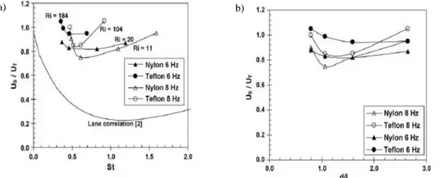
Studies were carried out to extend the experimental data on particle drag coefficients in free-stream turbulence, as a function of solid particles characteristics; in particular, the motion of different size particles made of Nylon and Teflon were examined in two different turbulent low fields, as shown in Fig.4.

Fig. 4 – Effect of turbulence on the settling velocity of Nylon and Teflon particles generated at oscillating frequencies of (a) 8Hz and (b) 6Hz which corresponded to r.m.s. turbulence velocities of 19.2 and 14.4 mm/s,

(19)

19

The results showed that the free-stream turbulence may lead to a significant reduction in settling velocity of solid particles, the function of particle characteristics as size and density. As Stokes number increases, 𝑈𝑠/𝑈𝑡 reduces, as it can be seen also from raising in particles’

diameter.

For higher Stokes numbers, and for particle’s diameter greater than the integral length scale of turbulence, the ratio of velocity tends to return to values around unity, for both materials. This trend is probably related to the fact that no turbulent eddies of enough size or energy deflect the particle from its path.

There was a considerable discrepancy between Lane’s correlation and the new experimental data obtained, as shown in Fig. 5(a).

Considering the correlation related to Lane et al. first study, new experiments carried out suggested that besides 𝑆𝑡 number, both 𝑑_𝑝/𝐿 and 𝑢₀/𝑈_𝑡 ratios needed to be considered as separate entities in developing a correlation for particle drag coefficient in turbulent flows.

Fig. 5 – (a) Comparing the experiment data for settling velocity of solid particles in turbulent flows with the model prediction of Lane et al. [11]. The results are presented as a function of Stokes and Richardson numbers. (b) The effect of particle size relative to the integral length scale of turbulence on the particle

settling velocity [8].

Fig. 5(b) suggests that the velocity curve starts to flatten as 𝑑𝑝/𝐿 reach the value of one. This

behaviour was found to be irrespective of the particle density or turbulence intensity. Furthermore, in Fig. 5(b), it seemed that minimum value, (𝑈𝑠/𝑈𝑡)min, for 𝑈𝑠/𝑈𝑡 occurred

around 𝑑_𝑝/𝐿 = 1 for all experimental tests.

b) a)

(20)

20

The most probable reason is that the maximum interaction between the particle and the turbulent vortices occur when particle size is approximately equal to the turbulence integral length scale.

Authors suggested that inertial force due to turbulence, and the net effective weight of the particles, due to the gravity, play a key role in describing the dimensionless ratio between velocities. For this reason, was defined as a parameter called Richardson number.

𝑅𝑖 =𝑔 |𝜌𝑝− 𝜌𝑓| 𝐿

𝜌_𝑓𝑢₀2 (1.14)

As shown in Fig. 6, a low value of Richardson number reflects the turbulence dominance. When Richardson number increases, the effect of turbulence on the settling velocity of particles reduces to negligible levels. Conversely, there appears to be a major effect on (𝑈𝑠/𝑈𝑡)min for low values of the Richardson number.

Fig. 6 – The maximum interaction between solid particles and turbulent eddies as a function of the Richardson number [8].

Concluding, particle density and turbulent intensity are the key parameters affecting the settling velocity, and from this, Richardson number is used to correlate the minimum reduction in the ratio between settling and terminal velocity, (𝑈_𝑠/𝑈_𝑡)min.

(21)

21

1.2.3 Brucato et al. (1998) - Magelli et al. (2008)

Brucato et al. and Magelli et al. studied the behaviour of solid particles in the agitated system, by proposing a correlation to calculate the effective settling velocity.

Initially, Magelli et al. (1990) proposed a correlation suggesting that the influence of turbulence on particle settling velocity, expressed in terms of the ratio between the settling velocity in the turbulent medium and that in still liquid, was a function of the ratio between particle diameter (𝑑_𝑝) and Kolmogorov scale of dissipative eddies (𝜆). The latter is expressed by: 𝜆 = (𝜈 3 𝜀) 1/4 (1.18)

where 𝜀 is the rate of kinetic energy dissipated per unit mass of fluid phase.

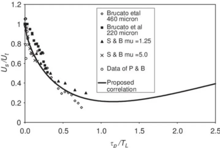
Data obtained from Magelli et al. study were gathered to indicating that the correlating parameter 𝜆/𝑑_𝑝 is related to the behaviour of the system. Unfortunately, those results did not fit well setting data used for the experiment, especially for the smallest glass beads, as it can be seen from Fig 7.

Fig. 7 – Comparison of experimental data with Magelli et al. (1990) experimental data (dots) and correlation. Glass beads (∆) 63-71 μm, (□) 212-250 μm, (○) 425-500 μm, silica (▪) 180-212 μm, (●) 425-500

(22)

22

Correlation proposed by Brucato et al. (1998) taken into consideration the reverse ratio proposed by Magelli et al. (1990) (i.e. 𝑑𝑝/𝜆). This term was directly correlated to the

normalized drag coefficient (𝐶𝐷) by a simple cube law.

𝒞𝒟 − 𝒞_𝒟𝑜 𝒞_𝒟𝑜 = 8.76 × 10 −4₍𝑑𝑝 𝜆 ) 3 (1.19)

Subsequently, studies by Magelli et al. were based on the measurement of vertical solid concentration profiles at steady-state conditions, as well as of local concentration transients, and interpreting the data with a simple phenomenological model along the same lines followed in the past with settling solids from Nocentini et al. and Pinelli et al., and the particles settling velocity was determined.

The study was performed in a high aspect ratio vessel agitated with multiple impellers; this configuration allows to magnify the vertical concentration gradients, and thus to make the analysis more reliable [8].

The solids distribution was usually characterised by limited radial concentration gradient; consequently, the vertical concentration profiles are their main distinctive feature, so this distribution in the stirred vessel was interpreted with a simple one-dimensional model. Using particles with density higher than the density of the fluid, by using non-dimensional coordinates for axis directed upwards, the dimensionless concentration under unsteady conditions, after an instantaneous injection at the base of the vessel, was calculated from a relationship, reported below.

𝐶∗(𝜁, 𝜃) = 𝑓 (𝑃𝑒𝑠, 𝜁) (1.20)

𝐶∗ _{= 𝐶/𝐶}

𝑎𝑣𝑔 𝑃𝑒𝑠 = 𝑈𝑠𝐻/𝐷𝑒𝑠 𝜃 = 𝑡𝐷𝑒𝑠/𝐻2

Where 𝐶∗, the dimensionless concentration, is a function of 𝑃𝑒_𝑠 and 𝜁. 𝐷_𝑒𝑠 is the dispersion coefficient and 𝑃𝑒𝑠 is the Peclet number for the solids: its value is positive for the buoyant

particles. 𝜁 is the dimensionless coordinate, while 𝐻 is vessel weight, and 𝜃 is the dimensionless time.

(23)

23

The particle rising velocity in the stirred tank was calculated from 𝑃𝑒𝑠 and dispersion

coefficient for the solid phase, considered equal to that for liquid phase, under steady-state measurement, 𝑈_𝑠 = 𝑃𝑒_𝑠𝐷_𝑒𝑠/𝐻. This was compared with terminal velocity (𝑈_𝑡), calculate with the Turton and Levenspiel’s correlation.

Settling velocity was found significantly lower than terminal velocity, as the influence of the turbulence on particle settling velocity was related to particles diameter (𝑑_𝑝) and Kolmogorov scale of dissipative eddies (𝜆).

The values of the ratio 𝑈𝑠/𝑈𝑡 of Magelli et al. obtained, were compared with empirical

correlation established for solid settling in a dilute, turbulent medium, as stated by Pinelli et al. (2001) and showed in Eq. (1.21).

𝑈𝑠

𝑈𝑡 = 0.4 ∙ 𝑡𝑎𝑛ℎ [16 𝜆

𝑑_𝑝− 1] + 0.6 (5)

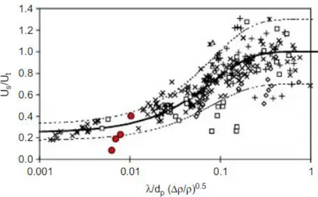
With the Kolmogorov scale of dissipative eddies (𝜆) given by the equation mentioned above. Studying the effects of particle inertia under conditions of isotropic turbulence, and by analysing bubble gas motion in a turbulent medium Oesterlè and Zaichik (2006), Doroodchi et al. (2008), Porte and Biesheuvel (2002) suggested considering particle-fluid interaction, in particular related to solid-to-liquid density.

Afterwards, studies carried out by Scargiali (2007) shown that introducing ratio between solid and fluid density reduced the average error of about 20% of the previous correlation (Eq. 1.22). The optimal exponent value for this ratio is equal to 0.5.

𝑈𝑠 𝑈𝑡 = 0.32 ∙ 𝑡𝑎𝑛ℎ [19 𝜆 𝑑_𝑝( 𝜌𝑠 − 𝜌𝑓 𝜌𝑓 ) 0.5 − 1] + 0.6 ₍₆₎

Eventually, Magelli et al. (2008) proposed a correlation to calculate 𝑈𝑠/𝑈𝑡, which contain

these two dimensionless parameters.

This correlation predicts solid distribution in processes where floating particles are dispersed in fluid, but it is possible to apply it also to describe gas-liquid systems, under idealised condition.

(1.21)

(24)

24 Eq. (1.22) is plotted in Fig. 8.

Fig. 8 – The ratio of the settling/rising velocity, 𝑈𝑠, in stirred systems to the terminal value, 𝑈𝑡, ●; buoyant

particles; other data points: settling particles (+××˖; Rushton turbines of three scales; ◊∆; PBT of two scales; □: A310 impellers) solid line: correlation for settling solids; dashed lines: ±30% of the correlation

line. [2]

According to Brucato et al. studies, one can see that as dimensionless terms on abscissa for the lowest and highest values date not converge. The ratio of the velocity 𝑈_𝑠/𝑈_𝑡 reaches a unitary value, as shown by the typical behaviour of a fluid at rest.

(25)

25

1.3 Analysis of correlations

The analysis performed by different authors underlines the limitations in their proposed correlations. In order to improve knowledge of the phenomenon, further studies should be necessary.

Spelt and Biesheuvel based their studies on investigating particles motion of equivalent diameter of about 1,0 mm, in isotropic turbulent flow and their data just covered range of 𝛽 ≪ 1. Therefore, the applicability of the correlation of Spelt and Biesheuvel is questionable for the turbulence of high intensity at small length scales.

Lane et al. in their studies considered Spelt and Biesheuvel dimensionless parameter 𝛽 and 𝜇∗, and combining both they obtained Stokes number.

Correlation proposed initially by Lane et al. was valid for 𝑆𝑡 < 0.7. By increasing Stokes number and particle diameter, 𝑈_𝑠/𝑈_𝑡 ratio decreases, reaching a minimum value for 𝑑_𝑝/𝐿 equal to one, corresponding to a maximum interaction between turbulence and particles. The 𝑈_𝑠/𝑈_𝑡 increases as the Stokes number increase as well, returning to a unity value at ratios 𝑑𝑝/𝐿 of more than 2.5.

Lane et al. intuited that the difference in density between fluid and particle was an important parameter in describing settling velocity. They used this parameter, through Richardson number, in order to establish the greatest contribution between gravity force domains respect to turbulence.

Magelli et al., according to Brucato et al., proposed a correlation by using a dimensionless parameter, 𝜆/𝑑𝑝. Unfortunately, the highest value of this reached a 𝑈𝑠/𝑈𝑡 unitary, as shown

by the typical behaviour of a fluid at rest.

In a second moment, Magelli et al. compared data with that of Pinelli et al., by concluding that the difference between particle and fluid density must be included in their correlation, with uncertainties regarding errors in measurement.

(26)

26

As suggested by Lane et al., the dimensionless parameters introduced by various authors should be considered as separate entities, in order to establish the exact relationship between them and particle settling velocity.

(27)

27

1.4 Kolmogorov Hypothesis

The first hypothesis that the disturbances in small scales in a turbulent fluid are approximately isotropic was found in the literature (Richardson in 1922), considering turbulence constituted by a set of disordered disturbances (eddies) that differ from each other in terms of size and scale.

Kolmogorov in 1941 stated that in the turbulent flow perturbations are characterized by the size of the vortex, and although it is a conceptual abstraction, its utility has greatly simplified the theoretical treatment and allows a better understanding of physics.

The energy terms involved in the motion of the fluid are characterized by instability mechanisms, that is the generation of vortices that over time generate ever-smaller vortices until the dimensions are not so small that the viscosity dissipates the structures preventing any further transfer.

Kolmogorov's hypothesis draws from the observation that the dynamics of turbulence depends on how quickly the energy is transferred from the large to the small scales and on the value of the viscosity that sets the wave number, to which the cut is made in the transfer of power. If the fluid dynamics phenomenon is statistically stationary, being the cascade from non-viscous energy, it is deduced that called the rate of turbulent kinetic energy (per unit of mass), (𝜀) produced in the unit of time transferred to the disturbances on a larger scale 𝐿, this will also be the energy dissipated in the unit of time.

Consequently, 𝜀 will be the characteristic of large scale of motions which will influence the statistical state of small scales fluctuations. The energy associated with them is of the order of 𝑢2_{and that the rate of kinetic energy dissipated will be}_{𝜀 ~ 𝜈}

𝐿3/𝐿, where 𝜈𝐿 is the

characteristic velocity related to a larger scale. At high Reynolds numbers, the direct dissipation of energy by the medium motion of the fluid under the action of the molecular viscosity is negligible, therefore the components of the instantaneous motion with relative fluctuations are considered:

(28)

28 𝜀 =1 2𝜈 ∑ ( 𝜕𝑢𝑖 𝜕𝑥_𝑗 + 𝜕𝑢_𝑗 𝜕𝑥_𝑖) ̅̅̅̅̅̅̅̅̅̅̅̅̅̅̅̅ 𝑖,𝑗 (7) 𝑢_𝑖 and 𝑢_𝑗 are the components of the instantaneous motion, in the direction i and j.

Kolmogorov claims that all the geometric information of the large vortices, determined by the average motion of the fluid, is lost. Consequently, the characteristics of small-scale motions must in a certain sense be universal, that is, similar for each high Reynolds number motion.

Considering the disturbances that have lost the directional property (anisotropy) of the average motion and are substantially isotropic, these will still have considerable dimensions and will have a characteristic size of the order of 𝐿. The description is given by Pope (2003), for the length of the scale 𝐿𝐸 (of the order of 1/6 𝐿), was useful as a demarcation between

the surely anisotropic vortices (𝑟 < 𝐿_𝐸) and the small locally isotropic vortices (𝑟 < 𝐿_𝐸). The properties of large-scale motions can influence the statistical properties of lower-scale disturbances only through the turbulent energy dissipation rate ε.

Furthermore, these properties must also depend on the parameters that characterize the physical properties of the fluid, which can be described by the density ρ and the viscosity ν. Since, however, the relative speed values are independent of the choice of the mass unit, the statistical properties of the motion of the disturbances cannot depend on ρ.

We can conclude that the statistical properties of disturbances on a sufficiently small scale will depend only on ε and ν.

Kolmogorov's first hypothesis:

In the case of disturbances in a sufficiently high Reynolds number field of motion, the probability distribution for velocities in a region of space-time where turbulence is locally isotropic is defined unambiguously by the values of 𝜀 and 𝜈.

Using variables such as the energy that dissolves (𝜀) and the viscosity that dissipates (𝜈), length scale is constructed dimensionally 𝜆, that is the magnitudes of these vortices, and the corresponding velocity and time 𝜏𝜆 of these vortices, as:

(29)

29 𝜈𝜆 = (𝜈 𝜀)1/4 (84) 𝜆 = (𝜈 3 𝜀 ) 1/4 (918) 𝜏_𝜆 = (𝜈 𝜀) 1/2 (1.25) With this observation we can understand Kolmogorov's first hypothesis which says: For sufficiently high Reynolds numbers, the characteristics of the small scales of all turbulent flows are universal and are determined by the viscosity and power dissipated. To quantify the dissipation scales was defined the Kolmogorov scales, that is the size, velocity and time, we define a Reynolds number equal to:

𝑅𝑒 =𝜈𝜆 𝜆

𝜈 = 1 (1.26)

Disturbances with a length of 𝜆 scale, characterized by a velocity 𝜈𝜆, have a number of

Reynolds equal to 𝑅𝑒 = 𝜈_𝜆 𝜆 /𝜈 = 1. 𝜆 is of the same order of magnitude as the scale length of higher-order disturbances on which viscosity still has an appreciable effect. Using the definition of 𝜆 it is possible to identify a dimensional range for the disturbances within which their main characteristic is local isotropy, in fact, all the disturbances with scale length 𝑟 lower than L and higher than Lam are locally isotropic.

The range 𝜆 − 𝐿_𝐸 is called: Universal Equilibrium Range.

Now consider the ratio between the scale length of the smallest motions 𝜆 and the scale length of the vertices of larger dimensions 𝐿 and the analogous ratios for the scale velocity and the characteristic scale time. These ratios are immediately determined by the definition of the Kolmogorov scale and by the fact that 𝜀 ~ 𝑈3/𝐿 in the following way:

𝜆 𝐿= 𝑅𝑒 −3/4 (1.27) 𝜈𝜆 𝑈 = 𝑅𝑒 −1/4 (1.28) 𝜏_𝜆 𝑇_𝐿 = 𝑅𝑒 −1/2 (1.29) (1.24) (1.18) (1.25) (1.26)

(30)

30

Hence, the Kolmogorov length decreases with increasing Reynolds number which characterizes the motion of the fluid and as well as the scaling speed and the scaling time, but more slowly. Therefore, at high Re values, the velocity and the characteristic time of scale of the smaller vortices (𝜈_𝜆 and 𝜏_𝜆) are small when compared with those of the larger vortices (𝑈, 𝑇𝐿).

In the case in which the Re value of the fluid motion is so high as to make 𝜆 assume a very small value if compared with 𝐿. In this type of turbulence, we can isolate a vast subset of disturbances of much smaller scale length 𝑟 of 𝐿 (and consequently homogeneous, isotropic and almost stationary) but a lot greater than the Kolmogorov length 𝜆. For these disturbances, the relative velocities 𝜈𝑟 will be much greater than 𝜈𝜆 and therefore the relative Reynolds

number 𝑅𝑒 = 𝜈_𝑟 𝑟 /𝜈 will be very high with respect to 𝑅𝑒 = 𝜈_𝜆 𝜆 /𝜈 = 1. In other words, in this dimensional subinterval, the dominant process is the inertial transfer of energy to small-scale disturbances, without however any appreciable conversion of energy directly into heat by the viscous forces. The statistical properties corresponding to this sub-range of scale (known as Inertial Range) therefore do not depend on the viscosity 𝜈.

This is Kolmogorov's Second Hypothesis:

In the case of turbulence with a sufficiently high Reynolds Re number, the multidimensional probability distribution for the velocities in a sufficiently small space and in intervals 𝑟 ≪ 𝐿 and 𝜏𝑘 ≪ 𝐿/𝑈 are determined, unambiguously, only by the value of the turbulent energy

dissipation rate 𝜀 and are independent of the viscosity 𝜈.

This description implies a cascade transfer through an energy flow that defines the average rate of kinetic energy dissipated (𝜀) from the largest scales of motion towards smaller and smaller ones up to the dissipative scales where viscosity transforms all energy into heat. This interval is called inertial because it does not depend on either forcing or dissipation (𝜈).

(31)

31

Fig. 9 – Kolmogorov hypothesis of the cascade of energy

Where 𝑇𝐿 = 𝐿/𝑈 is the time scale of large scale of flow.

Considering at this point an 𝐿_𝐷 scale length (𝐿_𝐷 = 60 𝜆) it is possible to divide the entire dimensional range in this way:

• Universal Equilibrium Range: 𝑟 < 𝐿_𝐸 • Inertial Range: 𝐿_𝐸 > 𝑟 > 𝐿_𝐷

• Dissipation Range: 𝑟 < 𝐿_𝐸

Fig. 10 – Division of dimensional range of turbulent disturbances

These relationships allow us to estimate the relationships between the characteristics of the largest and smallest scales in a turbulent flow as a function of the Reynolds number only. The dynamics of intermediate structures with dimension 𝑟 such that 𝐿 ≫ 𝑟 ≫ 𝜆 (or in time using “𝑠” such as 𝑇𝐿 ≫ 𝑠 ≫ 𝜏𝜆), was considered by Kolmogorov's third hypothesis inspired

by the observation that the dynamics of turbulence depends on how quickly energy is transferred from large to small scales and from the value of the viscosity that.

(32)

32

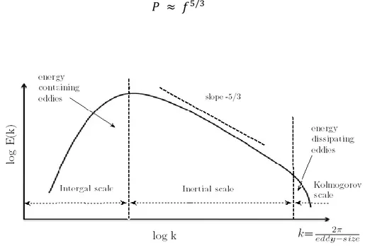
Introducing the wave number 𝑘 where the cut is made in the transfer of power, and considering that for sufficiently high Reynolds numbers the characteristics (the statistics) of the structures of dimension 𝑟 (with 𝐿 ≫ 𝑟 ≫ 𝜆) are universal and depend solely on 𝜀 (and therefore are independent of 𝜈), we can derive the famous power law (𝑘−5/3_{) for the energy}

spectrum:

𝐾 = ∫ 𝐸(𝑘)𝑑𝑘

∞

0 (100)

where 𝐾 is the kinetic energy per mass unit of the flow, from Kolmogorov's third hypothesis and from dimensional arguments we obtain:

𝐸(𝑘) = 𝒞 𝜀2/3_𝑘−5/3 _(1.31)

where 𝒞 is a universal constant.

Particularly, the power dissipated in the homogeneous and isotropic turbulence follows a power law of the type:

𝑃 ≈ 𝑓5/3 ₍₁₁₂₎

Fig. 11 – Kolmogorov hypothesis to the energy transferred from a bigger scale to a smaller one. (1.30)

(33)

33

Chapter II

− Motivation & Objectives

In the chemical industry, most of the processes involve mixtures of solid and fluid.

In these circumstances, the behaviour of solid particles in a turbulent fluid is not properly defined and further improvement would be necessary to the equipment design.

Several fundamental studies were carried out on the effects of the continuous phase acting on dispersed particles, but inconclusive results were reported, probably due to the limited experiment range of physical and operating conditions examined [13].

The multiphase flows involving a suspension of particles in the liquid were carried out under turbulent conditions of varying intensity in processing vessels, such as loop reactors and mechanically agitated vessels. Often in these processes, uniform dispersion of particles is achieved due to the interaction between turbulent eddies and the disperse phases. A better understanding of such interaction is fundamental to the effective design, modelling and operation of multiphase systems [6].

The difficulty in the modelling of the sedimentation, suspension and fluidisation phenomenon is related to the complexity of the structure formed by free-stream turbulence, which does not allow to predict the exact particles’ motion.

From a mathematical point of view, the detailed description of the transition from laminar to turbulent flow is a complex problem; as the Reynolds number increases, a laminar flow becomes unstable, consequently the possibility that small perturbations evolve in a chaotic manner giving rise to the turbulent motion.

A fluid exerts a drag force on the particle that can be calculated by Stokes' law, in cases of a regime of motion with low values of Reynolds. When Reynolds increases, Stokes' law is no longer valid, and consequently, the relationship between drag coefficient (𝐶_𝐷) and number of Reynolds is not linear.

Due to the underlying non-linear nature of turbulent flows and the fact that a larger number of particles are present, an analytical solution to the problem cannot be expected. A possible way to investigate the problem, in case of industrial interest, is to considerer a statistical

(34)

34

description of turbulent motion, based on the solution of a mediated equation using a Stochastic Differential Equation (SDE).

Langevin in 1908 proposed a Stochastic Differential Equation (SDE) to describe the homogeneous and isotropic turbulent flows. This has been used, in this works, to describe the fluid’ motion (§ 3.2).

The aim of this work is to define a correlation to describe the phenomenon of the particles settling, able to provide settling velocity data to compare with experimental data obtained from simulations.

The proposed correlation includes parameters that coming out from the previous studies mentioned above (§ 1.2). 𝑈_𝑠 𝑈𝑡= 𝑓 ( 𝑑𝑝 𝜎 𝑇_𝐿, 𝜎 𝑈_𝑡, Δ𝜌 𝜌_𝑓, 𝑡_𝑟 𝑇_𝐿, 𝑔 Δ𝜌 𝐿 𝜌_𝑓 𝜎 ) (12.1)

The final correlation will be better described in Chapter 4.

(35)

35

Chapter III

− Methodology

3.1 Introduction

Langevin dynamics has been used in this work to describe the random motion of the turbulent flow. This model is constituted by Stochastic Differential Equations (SDEs) that are differential equation in which one, or more, terms include a random variable. These terms represent stochastic processes or the probabilistic version of a dynamic system, allowing to quantify parameters varying in a causal manner over time.

By carrying out multiple tests, the most probable value of a random variable is identified by considering its mean with a gaussian trend, which is characterized with a relative index of deviation or standard deviation from the expected value.

In this work, homogeneous and isotropic turbulence with zero mean flow has been considered.

The turbulent motion in these conditions can only occur in the absence of physical boundary limits or externally imposed mean flows; the structure of the velocity field, in terms of statistical quantities, is invariant under translation (homogeneity) and rotation (isotropy) of the reference system, with respect to which the motion of the fluid is being described. Only in these conditions, the chaotic motion of the fluid can develop freely, according to the dynamics imposed by the equations of motion.

The conditions of homogeneous and isotropic turbulence are ideal, thus rarely occur in practical applications. It can be assumed that the structure formed in chaotic motion at sufficiently small scales, existing at high Reynolds number, in small regions of space and for short duration intervals, is practically homogeneous and isotropic.

Fluid’s motion can be described decomposing its instantaneous velocity in two terms, an average value and a fluctuation one.

(36)

36

By imposing stationarity for velocity’s average value, the signal can be expressed as:

𝑢(𝑥, 𝑡) = 𝑈(𝑥) + 𝑢′(𝑥, 𝑡) (13.1)

𝑈(𝑥) is the average value, while signal no-stationarity is given by fluctuation term 𝑢′_{(𝑥, 𝑡).}

Fig. 12 shows the decomposition of the signal in part medium and fluctuation.

Fig. 12 – Reynolds decomposition of a statistically stationary signal in part medium and part floating [12].

Fig. 13 – Decomposition of a statistically non-stationary signal in part medium and part floating [12].

If the average velocity is also a function of time, then the average operation should not be carried out for an infinite time, but over a finite interval which is very large compared to the time scales of the fluctuations, but rather short if compared with the times of variation of the mean-field (Fig. 13).

(37)

37

3.2 Langevin Equation

In the case of homogeneous, isotropic and statistically stationary turbulence by artificial force, the values of 𝜅 (kinetic energy) and 𝜀 (average rate of dissipated kinetic energy) are constant, with zero mean velocity. These premises allow to consider the particles of fluids all with the same characteristics, and it is, therefore, sufficient to consider a component of the velocity of the fluid particle 𝑈+(𝑡), seen as the composing of velocity with a Lagrangian point of view.

The Langevin equation considers the velocity of microscopic-sized fluid particles following a Brownian-like motion. The stochastic processes 𝑈∗(𝑡) obtained from the Langevin’ equation are called Ornstein-Unlenbeck (UO) processes, characterizing a Probability Density Function (PDF) [15].

Considering Eq.(3.2.1), the deviation 𝑢′_{presents an irregular, unpredictable trend and can}

be considered a random variable. It is possible to associate a difference density function 𝑝(𝑢′_{) to the gap such that the product 𝑝(𝑢}′_{)𝑑𝑢 represents the probability that the random}

variable 𝑢′ assumes the value between 𝑢′ and 𝑢′+ 𝑑𝑢′.

The probability 𝑃 that the random variable assumes a value within a finite range −𝑢₀′ ≤ 𝑢′ ≤ 𝑢₀′ will, therefore, be given by:

𝑃(𝑢′_{) = ∫ 𝑝(𝑢′)𝑑𝑢′} 𝑈0′

−𝑈0′

(3.2.1)

Referring to Fig.14, which shows a time course of a velocity difference, the interval of the values assumed by the difference must be divided into equal parts with an amplitude equal to ∆𝑢′_{. Subsequently, considering an interval of values of}_𝑢′_{prime between (𝑘 − 1)∆𝑢}′_e

𝑘∆𝑢′, it must quantify the interval of time during which the random variable assumes values included in that interval. Said 𝜏𝑘 this interval and 𝑇𝐿 the duration of the experiment or better

the time interval for which the stochastic process 𝑋(𝑡) loses correlation with the value possessed at the initial instant, the ratio 𝜏_𝑘/𝑇_𝐿 provides an approximate estimate of the probability that the variable 𝑢′ prime takes values between (𝑘 − 1)∆𝑢′ e 𝑘∆𝑢′.

(38)

38

Fig. 14 – Deviation of velocity during the time [9].

Consequently, the sum of all 𝜏_𝑘 is equal to the total duration of the experiment. This condition can be expressed by referring to the probability density estimate:

∑ ( 𝜏𝑘

𝑇𝐿 ∆𝑢′)

𝑘 ∆𝑢′ = 1 (142)

Knowing the probability density function (PDF) associated with the event in question, we can define the expected or average value of the random variable:

〈𝑢′〉 = ∫ 𝑢′ 𝑝(𝑢′) 𝑑𝑢′

∞

−∞ (3.2.3)

The expected value of the velocity difference is zero, in fact, by approximating the letter integral with a summation we have:

∑ 𝑢_𝑘′ 𝑘 ( 𝜏𝑘 𝑇𝐿 ∆𝑢′ ) ∆𝑢′= 1 𝑇𝐿 ∑ 𝑢_𝑘′ 𝑘 𝜏𝑘 _(3.2.4)

Where 𝑢_𝑘′ prime is the average value assumed by the velocity difference in the time interval 𝜏𝑘. The sum is made up of positive and negative products, which when added together give

zero results.

The expected value of the velocity 𝑢 obviously coincides with the average value 𝑈, introduced above.

(3.2.2)

(3.2.3)

(39)

39

𝜎2 = ∫ 𝑢∞ ′2 𝑝(𝑢′)𝑑𝑢′

−∞ (155)

The mean square deviation is defined as the quantity being diffusion processes not differentiable, the standard tools of differential calculus cannot be applied. Instead of differential calculus, the appropriate method is the Ito calculus; and, instead of being described by ordinary differential equations, diffusion processes are described by stochastic differential equations.

The infinitesimal increment of the process 𝑈(𝑡) is defined by:

𝑑𝑈(𝑡) = 𝑈(𝑡 + 𝑑𝑡) − 𝑈(𝑡) (166)

where 𝑑𝑡 is a positive infinitesimal time interval.

For the Wiener process, in particular, it possible to consider:

𝑑 𝑊(𝑡) = 𝑊(𝑡 + 𝑑𝑡) − 𝑊(𝑡) =⏞

𝐷

𝒩(0, 𝑑𝑡) (172.7)

The symbol =⏞

𝐷

is read as “is equal in distribution to”, and 𝒩(𝜇, 𝜎2) is the normal distribution, in particular, denotes the normal with mean 𝜇 and variance 𝜎2.

Now consider the process 𝑈(𝑡) defined by the initial condition 𝑈(𝑡_𝑜) = 𝑈𝑜 and by the

increment:

𝑑𝑈(𝑡) = 𝑎[𝑈(𝑡), 𝑡] 𝑑𝑡 + 𝑏[𝑈(𝑡), 𝑡] 𝑑𝑊(𝑡) (188) For given functions 𝑎(𝑉, 𝑡) and 𝑏(𝑉, 𝑡). It is readily verified that the process 𝑈(𝑡) defined by this stochastic differential equation is a diffusion process, and, as implied by the notation, the drift and diffusion coefficients are 𝑎(𝑉, 𝑡) and 𝑏(𝑉, 𝑡) [15].

A random variable is fully characterized by its probability density function (PDF), and two random variables with the same probability density function (PDF), are statistically identical. Similarly, a diffusion process is fully characterized by its drift and diffusion coefficients; and two diffusion processes with the same coefficients are statistically identical [15].

(3.2.5)

(3.2.6)

(3.2.7)

(40)

40

Thus, the stochastic differential equation Eq. (3.2.9) provides a general expression for a diffusion process. It shows that the infinitesimal increment of a diffusion process is Gaussian, i.e.,

𝑑𝑈(𝑡) = 𝒩(𝑎[𝑈(𝑡), 𝑡]𝑑𝑡, 𝑏[𝑈(𝑡), 𝑡]2_𝑑𝑡) ₍₁₉₉₎

This Gaussian is not a defining property of diffusion processes, but rather a deduction from their definition [15].

The Langevin equation denotes this velocity mentioned above as 𝑈∗_{(𝑡), thus obtaining:}

𝑑𝑈∗(𝑡) = −𝑈∗_(𝑡)𝑑𝑡 𝑇𝐿 + (2𝜎 2 𝑇𝐿 ) 1 2 𝑑𝑊(𝑡) (2010)

where 𝑇_𝐿 is the Lagrangian integral time-scale e 𝜎2_{is the variance, both constant.}

The Eq. 3.2.10 can be express through the finite-difference equation:

𝑈∗(𝑡 + ∆𝑡) = 𝑈∗_{(𝑡) − 𝑈}∗_(𝑡)∆𝑡 𝑇𝐿 + (2𝜎 2_∆𝑡 𝑇𝐿 ) 1 2 𝜉(𝑡) (2111)

Where the first term is related to the dissipation coefficient which causes the velocity to relax towards zero on the timescale 𝑇_𝐿, while the second term is called random coefficient and it is the statistical refers to a random increment to zero-mean of the standard deviation 𝜎2. The term 𝜉(𝑡) is the standardized Gaussian random variable, which is independent of itself at different times and which is independent of 𝑈∗_{(𝑡) at the last time.}

The constant diffusion coefficient:

𝑎(𝑈∗, 𝑡) = −𝑈

∗

𝑇_𝐿

(2212)

Considering the random coefficient 𝑑𝑊(𝑡) = 0, and integrating the Langevin equation:

∫ 𝑑𝑈∗ 𝑡 0 = − ∫ 𝑈 ∗ 𝑇_𝐿 𝑡 0 𝑑𝑡 ₍₂₃₁₃₎ 𝑙𝑛𝑈𝑡 ∗ 𝑈₀∗ = − 𝑡 𝑇𝐿 → 𝑈𝑡∗ = 𝑈0∗ 𝑒𝑥𝑝 (−𝑡/𝑇𝐿) ₍₂₄₁₄₎ (3.2.9) (3.2.10) (3.2.11) (3.2.12) (3.2.13) (3.2.14)

(41)

41

Which means that the velocity would be totally dissipated during the time (back curve in Fig. 15).

The constant diffusion coefficient:

𝑏(𝑈∗_{, 𝑡) = (}2𝜎 2

𝑇_𝐿 )

1

2 (2515)

The random coefficient implies that fluid has a random motion, with normal distribution 𝜎2_.

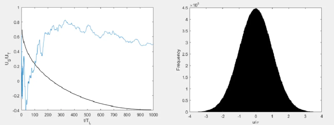
Fig. 15 – The right plot is the velocity of the fluid obtained by the Langevin equation, where the purple curve

is due to the dissipation term and the blue curve is due to the random term. At left the Gaussian curve of distribution velocity.

Plotting the Langevin equation is possible to evaluate that 𝑈∗_{is a statistically stationary and}

a Gaussian process, that is characterized with an average at zero, with variance 𝜎2_{and, in}

particular with an autocorrelation function given by:

𝜌(𝑠) = 𝑒−|𝑠|/𝑇𝐿 ₍₂₆₁₆₎

The autocorrelation function is the correlation of a signal with a delayed copy of itself as a function of delay. Informally, it is the similarity between observations as a function of the time lag between them.

(3.2.15)

(42)

42

If this is the autocorrelation function of the Lagrangian velocity, its Lagrangian integral timescale is defined by:

𝑇_𝐿 = ∫ 𝜌(𝑠)𝑑𝑠

∞

0 (2717)

If the equation relatives at autocorrelation function are consistent with this definition the 𝑇_𝐿 the coefficient in the Langevin equation is indeed the integral timescale of the process. The Langevin equation is correct in yielding a Gaussian probability density function (PDF) of velocity. In isotropic turbulence, the one-time PDF of the Lagrangian velocity 𝑈+(𝑡) is identical to one-point, one-time Eulerian PDF as demonstrated from experiment and DNS (direct numeric simulation), where PDF’s are very close to Gaussian [15].

The correct variance is defined by:

𝜎2 =2 3𝜅

(2818)

Considering high-Reynolds number of turbulence in which there is a large separation between the integral timescale 𝑇𝐿 and the Kolmogorov time scale 𝜏𝜂, it has been examined

𝑈+(𝑡) on inertial-range timescales “𝑠”, 𝑇𝐿 ≫ 𝑠 ≫ 𝜏𝜆. This is best done through the

second-order Lagrangian Structure Function:

𝐷𝐿(𝑠) ≡ 〈 [𝑈+(𝑡 + 𝑠) − 𝑈+(𝑡)]2〉 (2919)

With this function, which is just the variance of the increment over the time interval 𝑠 > 0, it is possible to express the autocorrelation of the velocity of a particle, and, particularly, being Lagrangian, it follows the trajectory of a particle taken individually.

The second-order Lagrangian Structure Function 𝐷_𝐿, for Kolmogorov's hypothesis, is proportional to “𝑠” in the inertial range, and also at the rate of dissipation of the turbulent kinetic energy as follows:

𝐷𝐿(𝑠) = 𝐶𝑜 𝜀 𝑠 per 𝑇𝐿 ≫ 𝑠 ≫ 𝜏𝜆 (3020)

Where 𝐶_𝑜 is the Kolmogorov constant, whereas the Langevin equation yields:

𝐷𝐿(𝑠) ≡ 〈 [𝑈∗(𝑡 + 𝑠) − 𝑈∗(𝑡)]2〉 (3121) (3.2.17) (3.2.18) (3.2.19) (3.2.20) (3.2.21)

(43)

43 = 2𝜎2

𝑇𝐿 𝑠 for 𝑠 ≪ 𝑇𝐿

(3222) Thus, the Langevin equation is consistent with the Kolmogorov hypothesis in yielding a linear dependence of 𝐷_𝐿 on “𝑠” in the inertial range.

In place of 𝜎2 e 𝑇_𝐿, in the Langevin equation, it is possible to use the terms kinetic energy (𝜅) and an average rate of dissipated kinetic energy (𝜀) and introducing the Langevin-model constant 𝒞_𝑜 through the relation:

2𝜎2 𝑇𝐿 = 𝒞𝑜 𝜀 (3323) 𝑇𝐿−1= 𝒞_𝑜 𝜀 2 𝜎2 = 3 4 𝒞𝑜 𝜀 𝜅 (3424)

Defined those constant, it has been used again to express the Langevin equation as: 𝑑𝑈∗(𝑡) = −3 4 𝒞𝑜 𝜀 𝜅 𝑈 ∗_{(𝑡) 𝑑𝑡 + (𝒞} 𝑜 𝜀) 1 2 𝑑𝑊(𝑡) (3525)

It is straightforward to incorporate Reynolds-number dependence in the Langevin model simply by making the model coefficient 𝒞_𝑜 depend on 𝑅𝑒_𝑇, therefore, 𝒞_𝑜(𝑅𝑒𝑇). Consistency

with the Kolmogorov hypotheses requires only:

𝑙𝑖𝑚

𝑅𝑒𝑇 → ∞

𝒞_𝑜(𝑅𝑒_𝑇) = 𝐶_𝑜 (3626)

where now we distinguish between the Kolmogorov constant 𝐶𝑜 and the model coefficient

𝒞𝑜(𝑅𝑒𝑇). Furthermore, 𝒞𝑜(𝑅𝑒𝑇) can be determined directly from DNS data by Eq.33, that

can be reorganized as:

𝒞𝑜= 4 𝜅 3 𝜀 𝑇𝐿 (3727) (3.2.22) (3.2.23) (3.2.24) (3.2.25) (3.2.26) (3.2.27)

(44)

44

Fig. 16 – The Langevin-model constant 𝐶𝑜 against Reynolds number. Symbols (●) from Eq.2*; Empirical fit

(▬) from Eq. 38.

The values of 𝒞_𝑜 were obtained from Direct Numerical Simulation (DNS), compared to the empirical fit, which is based on a suggestion by Sawford et al. [16].

𝒞_𝑜(𝑅𝑒_𝑇) = 6.5

(1 + 140 𝑅𝑒𝑇−4/3)3/4 (3828)

From Fig. 16, the fit represents the data which is consistent with the Kolmogorov hypotheses with 𝐶_𝑜 = 6,5. 𝜎 = √ 2 3𝑘 (3929) 𝑅𝑒𝑇 = √ 15 𝜎 𝜀 𝜇 𝜌 (4030)

𝑅𝑒_𝑇 is the Taylor-Scale Reynolds number which is sometimes called the turbulence length scale, is a length scale used to characterize a turbulent fluid flow. The Taylor microscale is the intermediate length scale at which fluid viscosity significantly affects the dynamics of turbulent eddies in the flow.

𝑇_𝐿−1=3 4 𝒞𝑜 𝜀 𝜅 (4131) (3.2.28) (3.2.29) (3.2.30) (3.2.31)