POLITECNICO DI MILANO
Dipartimento di Chimica, Materiali
e Ingegneria Chimica “Giulio Natta”
Analysis of the gas phase Kinetics Active
during InN Deposition from 𝐍𝐇
𝟑and In(CH3)3
Supervisor: Prof. Carlo Cavallotti
Master Thesis of:
Mattia Maggioni
Matricola 858959
3
POLITECNICO DI MILANO
Dipartimento di Chimica, Materiali
e Ingegneria Chimica “Giulio Natta”
Analysis of the gas phase Kinetics Active
during InN Deposition from 𝐍𝐇
𝟑and In(CH3)3
Supervisor: Prof. Carlo Cavallotti
Master Thesis of:
Mattia Maggioni
Matricola 858959
4
Ringraziamenti
Voglio ringraziare il Politecnico di Milano per i mezzi e la conoscenza messa a disposizione per svolgere questo studio; ringrazio il Prof. Cavallotti per la pazienza e la passione che mi ha trasmesso per questo campo di studi, sin dal corso di ACK.
Un ringraziamento particolare va a tutti coloro che mi sono stati vicini e mi hanno supportato e sopportato in questo periodo di gestazione della tesi, Annarella, Alessandro e Marianna, ringrazio Cristina per la vicinanza, la testardaggine e l’affetto.
Ringrazio Marcello e Luigi, compagni di tesi e di studi quantomeccanici, e Aldo, per i progetti e il buon tempo passato assieme. Grazie a Matteo per i consulti a tarda ora da Montpellier per risolvere i problemi tecnici.
Complicare è facile, semplificare è difficile Bruno Munari
5
Sintesi
In questa tesi di laurea è stato affrontato il problema della definizione di uno schema cinetico relativo alla descrizione di un sistema reagente composto da Indio trimetile e ammoniaca in un ambiente inerte di idrogeno. A tale scopo sono stati implementati calcoli quantomeccanici per ricavare tutti i parametri termodinamici necessari a descrivere le specie coinvolte nello schema cinetico utilizzando diversi possibili accoppiamenti tra livelli di teoria e basis sets: m062x, wb97xd e b3lyp sono state le approssimazioni teoriche utilizzate, mentre sdd, lanl2dz e crenbl sono stati i basis sets utilizzati, in diverse combinazioni. È stato poi scelto il migliore accoppiamento basandosi su un confronto tra le energie di legame per le specie coinvolte calcolate nelpresente lavoro e la letteratura scientifica. Una volta selezionata da un confronto con la letteratura scientifica la migliore base di dati,
successivamente a partire da questi sono stati svolti calcoli per determinare la composizione all’equilibrio del sistema reagente, e a seguire sono state
calcolate le velocità di reazione necessarie a definire in modo accurato la cinetica del sistema reagente. Le reazioni dirette e inverse proposte sono poi state analizzate considerando la natura delle strutture attraverso cui la
reazione evolve e la consistenza dei risultati rispetto ai calcoli di composizione all’equilibrio fatta nei punti precedenti.
6
Abstract
In this thesis has been faced the problem related to the definition of a kinetic scheme that can effectively describe a reacting system composed by trimethyl Indium and ammonia in an inert atmosphere of hydrogen. To do this has been implemented quantum mechanics calculations to evaluate all thethermodynamic parameters necessary to describe all the species involved in the kinetic scheme using different possible couplings between theory
approximation levels and basis sets: m062x, wb97xd and b3lyp has been the theoretical approximation used, while sdd, lanl2dz and crenbl has been the basis sets used in different combinations. After that I choose the best coupling comparing bond energies of the species involved in the scheme calculated in this job with the experimental literature. A comparison between single results and scientific literature values has been done and I selected the best set of data, using them as a base for successive calculations of equilibrium
composition for the reacting system. After that all the reaction rates that accurately define the kinetics of the reacting system have been calculated. For all the reactions involved in the scheme have been calculated the direct and related inverse transformation velocity, with a perfect match with equilibrium calculations evidence.
7
Content index
Ringraziamenti ………4 Sintesi………5 Abstract………6 Content index………7 Figures index………..………..9 Table index………11 1. Chapter 1: Introduction ……….131.0. InGaN: description and applications………13
1.1. CVD………..17
1.2. InGaN crystals growth………..18
1.3. CVD modeling………21
1.4. State of the art of Thermodynamics………..23
1.5. Aim of the Thesis……….24
2. Chapter 2: Quantum Chemistry……….25
2.0. Schroedinger equation and wave function………25
2.1. Born-Oppenheimer approximation ……….27
2.2. Hartree Product ………..29
2.3. Slater determinant……….30
2.4. Hartree Fock Approximation………31
2.5. Density Functional Theory……….32
2.6. Basis Sets……….37
2.7. Hindered Rotors………..40
2.8. Thermodynamic properties from Gaussian09 data……….44
2.9. Equilibrium calculations……….49
2.10. Transition state theory……….50
3. Chapter 3: Results……….55
3.0. Description……….55
3.1. Properties calculations……….55
3.2. Equilibrium calculations……….71
8
4. Chapter 4: Conclusions…………..………..122 Appendix 1……….123 References………..148
9
Figures index
Figure 1.1 Conductors, semiconductors and insulators valence and conduction bands. Figure 1.2 InGaN based diode illustration.
Figure 1.3 CVD deposition scheme.
Figure 2.1 Example of rotational PES for the amino group rotations along the In – NH2 bonds for In(NH2)3.
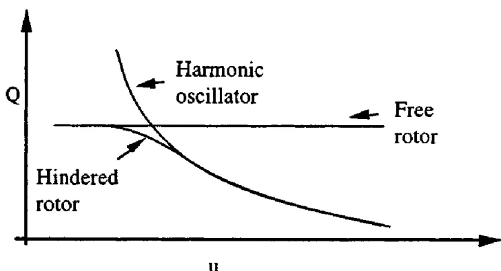
Figure 2.2 Differences between a free rotor, a harmonic oscillator and an hindered rotor.
Figure 2.3 Example of potential energy surface profile for a reaction, the progress of the reaction is described along the reaction coordinate, which usually is a length.
Figure 2.4 Two different types of reactions: a tight transition state reaction on the left and a loose profile transition state reaction on the right.
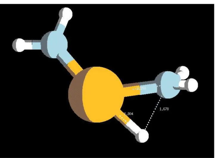
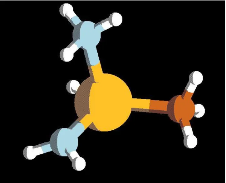
Figure 3.1 In3(NH)3H3 molecule. Figure 3.2 In3(NH)3(NH2)3 molecule. Figure 3.3 In2NH(CH3)2NH2H molecule.
Figure 3.4 Equilibrium composition for several gas phase species expected to play a role in GaN MOVPE. Calculations performed at constant T, at the pressure of 0.2 bar, and for the following global gas phase composition: 0.25 for NH3, 0.7495 for H2 and 0.0005 for trimethyl gallium.
Figure 3.5 Equilibrium composition for several gas phase species expected to play a role in InN MOVPE. Calculations performed at constant T, at the pressure of 0.2 bar, and for the following global gas phase composition: 0.25 for NH3, 0.7495 for H2 and 0.0005 for trimethyl indium.
Figure 3.6 Equilibrium composition for several gas phase species expected to play a role in InN MOVPE. Calculations performed at constant T, at the pressure of 0.2 bar, and for the following global gas phase composition: 0.25 for NH3, 0.7495 for H2 and 0.0005 for trimethyl indium.
Figure 3.7 Equilibrium composition for several gas phase species expected to play a role in GaN MOVPE. Calculations performed at constant T, at the pressure of 0.2 bar, and for the following global gas phase composition: 0.25 for NH3, 0.7495 for H2 and 0.0005 for trimethyl gallium.
Figure 3.8 Equilibrium composition for several gas phase species expected to play a role in InN MOVPE. Calculations performed at constant T, at the pressure of 0.2 bar, and for the following global gas phase composition: 0.25 for NH3, 0.7495 for H2 and 0.0005 for trimethyl indium.
Figure 3.9 Equilibrium composition for several gas phase species expected to play a role in GaN MOVPE. Calculations performed at constant T, at the pressure of 0.2 bar, and for the following global gas phase composition: 0.25 for NH3, 0.7495 for H2 and 0.0005 for trimethyl gallium.
Figure 3.10 Equilibrium composition for several gas phase species expected to play a role in InN MOVPE. Calculations performed at constant T, at the pressure of 0.2 bar, and for the following global gas phase composition: 0.25 for NH3, 0.7495 for H2 and 0.0005 for trimethyl indium.
Figure 3.11 Rotational PES for methyl group rotation along the bond In – CH3 inside In(CH3)3. Figure 3.12 Rotational PES for amino group rotation along the bond In – NH2 inside In(CH3)2NH2. Figure 3.13 Rotational PES for methyl rotation along the bond In – CH3 inside In(CH3)2NH2. Figure 3.14 Transition state geometry for the reaction of the paragraph.
10
Figure 3.16 Transition state geometry for the reaction of the paragraph.
Figure 3.17 Rotational PES for amino group rotation along the bond In – NH2 inside In(NH2)3. Figure 3.18 Transition state geometry for the reaction of the paragraph.
Figure 3.19 Rotational PES for methyl group rotation along the bond In – CH3 inside InCH3NH2H. Figure 3.20 Rotational PES for amino group rotation along the bond In – NH2 inside InCH3NH2H. Figure 3.21 Transition state geometry for the reaction of the paragraph.
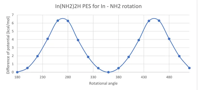
Figure 3.22 Rotational PES for amino group rotation along the bond In – NH2 inside In(NH2)2H. Figure 3.23 Transition state geometry for the reaction of the paragraph.
Figure 3.24 Transition state geometry for the reaction of the paragraph. Figure 3.25 Transition state geometry for the reaction of the paragraph. Figure 3.26 Transition state geometry for the reaction of the paragraph. Figure 3.27 Transition state geometry for the reaction of the paragraph. Figure 3.28 Transition state geometry for the reaction of the paragraph.
Figure 3.30 Rotational PES for amino groups rotation along the bond In – NH2 inside In2NHH2(NH2)2. Figure 3.31 Transition state geometry for the reactant well for the reaction of the paragraph.
Figure 3.32 Transition state geometry for the transition state of the reaction of the paragraph. Figure 3.33 Transition state geometry for the product well for the reaction of the paragraph.
11
Tables index
Table 2.1 Thermochemical data calculated from Gaussian 09 output file: an example based on In(CH3)2NH2 case.
Table 3.0.1 Results for m062x level of approximation of theory executed with Gaussian 09 on Indium based species with lanl2dz and sdd basis sets expressed in Hartree.
Table 3.2 Results for b3lyb level of approximation of theory executed with Gaussian 09 on Indium based species with lanl2dz and sdd basis sets, expressed in Hartree.
Table 3.3 Results for wb97xd level of approximation of theory executed with Gaussian 09 on Indium based species with lanl2dz and sdd basis sets, expressed in Hartree.
Table 3.4 Comparison between bond energies obtained with m062x and lanl2dz sdd basis sets calculations and Skulan et al. bond energies, marked as Literature true value, all the data are expressed in kcal/mol. Table 3.5 Comparison between bond energies obtained with b3lyp and lanl2dz sdd basis sets calculations and Skulan et al. bond energies, marked as Literature true value, all the data are expressed in kcal/mol. Table 3.6 Comparison between bond energies obtained with wb97xd and lanl2dz sdd basis sets calculations and Skulan et al. bond energies, marked as Literature true value, all the data are expressed in kcal/mol. Table 3.7 Results for wb97xd level of approximation of theory executed with Gaussian 09 on Indium based species with a custom crenbl basis sets, expressed in Hartree.
Table 3.8 Comparison between bond energies obtained with wb97xd and crenbl basis sets calculations and Skulan et al. bond energies, marked as Literature true value, all the data are expressed in kcal/mol. Table 3.9 Calculated energies and entropies for all the chemical species analyzed, is also reported if available the literature respective data, calculated with wB97XD/SDD.
Table 3.10 Enthalpies of formation at 298 K and 1 atm for all the species analyzed in the scheme with the respective reactions used to estimate the parameters, calculated with wB97XD/SDD.
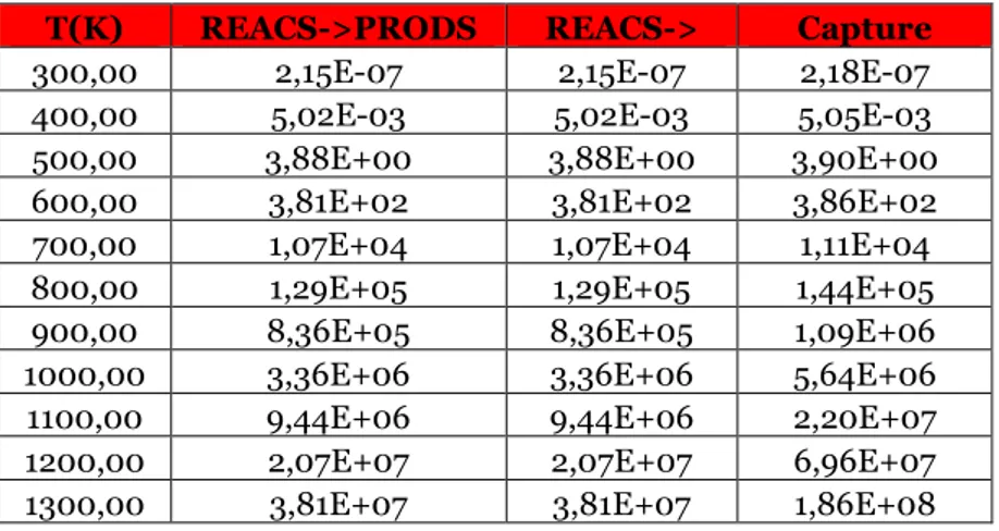
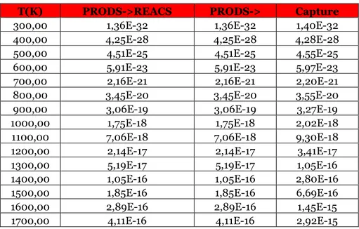
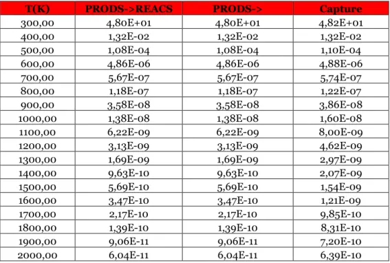
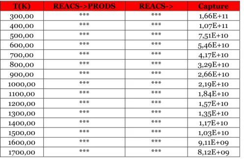
Table 3.11 Reaction rates for the direct reaction treated in the paragraph for different temperature values at 1 atm, expressed in cm^3/s.
Table 3.12 Reaction rates for the inverse reaction of the paragraph for different temperature values at 1 atm, expressed in cm^3/s.
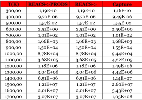
Table 3.13 Reaction rates for the direct reaction treated in the paragraph for different temperature values at 1 atm, expressed in cm^3/s.
Table 3.14 Reaction rates for the inverse reaction of the paragraph for different temperature values at 1 atm, expressed in cm^3/s.
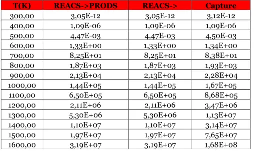
Table 3.15 Reaction rates for the direct reaction treated in the paragraph for different temperature values at 1 atm, expressed in cm^3/s.
Table 3.16 Reaction rates for the inverse reaction of the paragraph for different temperature values at 1 atm, expressed in cm^3/s.
Table 3.17 Reaction rates for the direct reaction treated in the paragraph for different temperature values at 1 atm, expressed in cm^3/s.
Table 3.18 Reaction rates for the inverse reaction of the paragraph for different temperature values at 1 atm, expressed in cm^3/s.
Table 3.19 Reaction rates for the direct reaction treated in the paragraph for different temperature values at 1 atm, expressed in 1/s.
12
Table 3.20 Reaction rates for the inverse reaction of the paragraph for different temperature values at 1 atm, expressed in cm^3/s.
Table 3.21 Reaction rates for the direct reaction treated in the paragraph for different temperature values at 1 atm, expressed in cm^3/s.
Table 3.22 Reaction rates for the inverse reaction of the paragraph for different temperature values at 1 atm, expressed in cm^3/s.
Table 3.23 Reaction rates for the direct reaction treated in the paragraph for different temperature values at 1000 atm, expressed in cm^3/s.
Table 3.24 Reaction rates for the inverse reaction of the paragraph for different temperature values at 1000 atm, expressed in cm^3/s.
Table 3.25 Reaction rates for the direct reaction treated in the paragraph for different temperature values at 1 atm, expressed in 1/s.
Table 3.26 Reaction rates for the inverse reaction of the paragraph for different temperature values at 1 atm, expressed in cm^3/s.
Table 3.27 Reaction rates for the direct reaction treated in the paragraph for different temperature values at 1 atm, expressed in 1/s.
Table 3.28 Reaction rates for the inverse reaction of the paragraph for different temperature values at 1 atm, expressed in cm^3/s.
Table 3.29 Reaction rates for the direct reaction treated in the paragraph for different temperature values at 1 atm, expressed in cm^3/s.
Table 3.30 Reaction rates for the inverse reaction of the paragraph for different temperature values at 1 atm, expressed in cm^3/s.
Table 3.31 Reaction rates for the direct reaction treated in the paragraph for different temperature values at 1000 atm, expressed in cm^3/s.
Table 3.32 Reaction rates for the inverse reaction of the paragraph for different temperature values at 1000 atm, expressed in cm^3/s.
Table 3.33 Reaction rates for the direct reaction treated in the paragraph for different temperature values at 1 atm, expressed in cm^3/s.
Table 3.34 Reaction rates for the inverse reaction of the paragraph for different temperature values at 1 atm, expressed in cm^3/s.
Table 3.35 Reaction rates for the direct reaction treated in the paragraph for different temperature values at 1 atm, expressed in 1/s.
Table 3.36 Reaction rates for the inverse reaction of the paragraph for different temperature values at 1 atm, expressed in cm^3/s.
Table 3.37 Reaction rates for the direct reaction treated in the paragraph for different temperature values at 10000 atm, expressed in 1/s.
Table 3.38 Reaction rates for the inverse reaction of the paragraph for different temperature values at 10000 atm, expressed in cm^3/s
Table 3.39 Preexponential factors k0 and activation energies for the direct and the inverse reactions analyzed in Section 3.
13
CHAPTER 1
INTRODUCTION
1.0. InGaN description and applications
What we are going to do is to model a system in which a chemical vapor deposition is taking place, from trimethyl Gallium and trimethyl Indium species mainly.
Chemical Vapor deposition is a process used to form a thin solid surface in which the product is deposed after that a reaction takes place in gaseous phase [3]. Industrially this process has applications in various fields, like the production of semiconductors, super conductors, insulating films and more. In our case we are going to produce InGaN from trimethyl Gallium and trimethyl Indium species, in a gaseous stream which has been added ammonia and molecular hydrogen as an inert specie.
Indium Gallium nitride (InGaN) is a semiconductor material made of a solid mixture of Gallium nitride and Indium nitride (GaN and InN), and is a direct bandgap semiconductor. A semiconductor is a material which has a value of electrical conductivity which is between the values assumed by a conductor and an insulator. A conductor is a specie which allow an electrical current to flow through it, so will have a high electrical conductivity, oppose to that we have an insulator, which is a material that doesn’t allow the free flow of
electrical charges in it, leading to a low electrical conductivity. Both the types of material are characterized by the presence of two “bands”, that are the valence band and the conduction band, which has different functions: the valence band is the band in which are contained the electrons of the specie when the material is not excited, the conduction band is the band in which the electrons of the material come once they are excited and the material is in the conductive phase [4]. For the conductive materials the two band are adjoining each other, and in some cases are partially superimposed, so that means that we will have to provide a small quantity of electrical current to let the material conduce, instead for the insulating materials the two band are far each other, that means that the electrons of the valence band will never reach
14
spontaneously the conductive band, so to make an insulator conduct an insignificant current we should spend a significative quantity of energy. The minimal energy state in the conduction band and the maximal energy state in the valence band are each characterized by a certain crystal
momentum (called k-vector) in the Brillouin zone (the uniquely defined primitive cell in the space of the cells that compose a material).
A direct band gap semiconductor is characterized by two equal k- vectors, while in the opposite case if these two vectors are different we will have an indirect band gap semiconductor.
Figure 4.1 Conductors, semiconductors and insulators valence and conduction bands
This material behavior of conductor is increased with the increase of the quantitative of indium in the alloy, which decreases the bandgap span from 3.4 eV (GaN value) to 0.69 eV (InN value) [5]. The ratio between In and Ga is usually between 0.02/0.98 and 0.3/0.7. InGaN is used nowadays to produce the light emitting layer of modern blue and green leds (light emitting diodes), and due to its high heat capacity and radiations sensibility is used also for solar photovoltaic devices (an important and relevant application is done for satellites arrays for example, and of course also in normal photovoltaic panels can be used this material).
15
Figure 1.5 InGaN based diode illustration
III-nitrides have already been proven to be an excellent material system for optoelectronic devices. While high-efficiency light-emitting diodes and lasers have been demonstrated, many of these material system properties are also of interest for PVs. It is known that InGaN alloys have a direct bandgap
semiconductors behavior, high adsorption coefficients and an excellent irradiance resistance, which make them good materials for solar cells, due to the fact that this material has a range of energies from 0.69 to 3.4 eV, that covers the solar radiation energy range. It’s been also shown that the optical and electronic properties of InGaN alloys exhibit a much higher resistance to high energy photon irradiation than currently used PV materials (such as GaAs and GaInP), and therefore offer a great potential for a radiation hard high efficiency solar cell for space applications. Furthermore, InGaN offers high carrier mobility, high drift velocity, high thermal conductivity, and high temperature resistance, which will all contribute to the realization of high efficiency solar cells for potential use under concentrate sunlight, which means also to space uses [6].
Usually a diode is an artifact made of two terminals which is used to conduct electricity to produce a colored light, that is a visible radiation that has a proper frequency. In fact, the visible light is a radiation which has a wave length between 390 nm and 700 nm (corresponding to a red light in the first case and to a blue/violet light in the second). Every material used to produce a conductor, or a semiconductor has a characteristic wave length field
included inside the visible light range, which depends on the electronic structure of the atoms and molecules involved.
In particular the material we are treating in this job is used to produce LEDs, which are light emitting diodes, which are two leads semiconductors light
16
sources. When a suitable voltage is applied to the leads, electrons are able to recombine with electron holes within the device, releasing energy in the form of photons (light radiations), and this phenomenon is called
electroluminescence. The color of the light emitted (so the characteristics of the radiation) depends on the band gap between the two types of band (valence and conduction band). These devices consist usually in a chip of a semiconductor material doped with impurities to create a p-n junction (a junction between two different types of semiconductor materials, one of which is considered the “positive” site due to the fact that it contains an
excess of holes while the “negative” side contains an excess of electrons). The electrical flux passes through the anode (p site) and is carried to the cathode (n site), and does not flow in the opposite direction. Photons are produced when an electron of the current flow reach a hole in the anode structure, due to the fact that this electron falls into a lower energy level and releases energy in form of photon. As told before the wavelength depends on the materials used to produce the led, in particular depends on the type of anode and cathode materials and on their band gap.
The emitted light wavelength can be controlled by the Ga/In ratio, it’s known that at 0.02/0.98 rate the emitted radiations are in the range of near
ultraviolet, at 0.1/0.9 the light wavelength is of 390 nm, at 0.2/0.8 the
radiation is violet blue with a wavelength around 420 nm, and at the limit of 0.3/0.7 the wavelength is 440 nm and the radiation is blue.
Now let’s treat all the specifics of Indium and Gallium nitrides, concerning their safety schedules.
Indium nitride at room conditions is a metal which melts at 1100°C with a low specific heat (0.32 J/g/°C and a low thermal conductivity (0.45 W/cm/°C). This material may cause irritation to the skin, the eye and no sensitizing effect are known. Being exposed to indium compounds may cause pain in the joints and bones, tooth decay, nervous and gastrointestinal disorders, heart pain and general debility. Exams with animals has been carried out, but the acute and chronic toxicity of this material has not been fully investigated yet. No relation between this material and cancer formations is available. [7]
Gallium nitride at room conditions is a solid and melts at temperatures over 2500°C with a low specific heat (0.49 J/g/°C and a low thermal conductivity (1.3 W/cm/°C). It may cause an allergic skin reaction, and between the safety precautions is suggested to not breath GaN dust, to avoid contact with skin and with eyes. [8]
17
1.1.
Chemical Vapor Deposition
To realize the process the reactive gases are introduced into the controlled environment of a reactor chamber where the substrates on which deposition takes place are positioned. The energy required to drive the chemical
reactions can be supplied thermally by heating the gas phase and growth surface (thermal CVD), but also by supplying photons in the form of, e.g., laser light to the gas (photo CVD), or through the application of an electrical discharge (plasma CVD or plasma enhanced CVD). The gas species fed into the reactor and the reactive intermediates created in the gas phase diffuse toward and adsorb onto the solid surface [3].
In CVD, physical and chemical processes take place at greatly differing time and length scales, which are usually classified using the scheme shown in Figure 2. Chemical reactions occurring in the gas phase and at the film
surface take place at the atomistic scale and are responsible for the formation of the gas phase precursors to the film growth, their rate of adsorption on the film surface, and the rate of incorporation of eventual dopants. [3]
At the microscale the surface species diffuse on the growth surface to nucleate islands or get inserted in the moving terrace steps. The microscale surface dynamics determines the morphology (epitaxial, polycrystalline, amorphous) of the film.
At the mesoscopic (i.e., micrometer) scale, free molecular flow and Knudsen diffusion phenomena in small surface structures determine the conformality of the deposition. Mesoscale phenomena can be of particular importance in patterned substrates.
At the macroscopic (i.e., reactor) scale, gas flow, heat transfer, and species diffusion determine temperature, composition, and flow fields throughout the reactor, which are eventually responsible of the film uniformity and growth rate.
Ideally, a CVD model should consist of a set of equations describing all the relevant macroscopic, mesoscopic, microscopic, and atomistic
physicochemical processes in the reactor and should be able to relate all these phenomena to the properties of interest of the deposited film. Unfortunately, this is not possible with the available modeling approaches, mostly because of the great difference in length and time scales between the involved
phenomena. Several alternative approaches are possible. The most adopted consists in the use of a coupled heat, mass, and momentum transport model
18
(briefly coupled transport model), which is formed by a set of partial
differential equations with appropriate boundary conditions, apt to describe the gas flow and the transport of energy and species in the reactor at the
macroscopic scale. This model can bridge the reactor-atomistic length scale as it can directly take as input kinetic constants of gas phase and surface
reactions determined using an atomistic approach. The properties of the gas mixture appearing in the transport model can be predicted with the kinetic theory of gases, while thermodynamic parameters can be found in the literature or estimated with thermochemical methods [9].
1.2. I
nGaN crystals growth
Once the reaction in the gaseous phase is carried out the nitrides produced can diffuse from the gaseous phase to the solid phase and deposit on the support; then the InGaN adsorbed on the surface can agglomerate with other InGaN molecules to form embryos, that are bigger agglomerates, instead embryos can also dissolve, and the nitrides can desorb from the solid surface and be released in the gaseous stream. If the embryos grow increasing the number of units of nitrides they can form crystals, which are the smallest units which cannot dissolve but can only grow. According to Yam and Hassan as the growth temperature is reduced, desorption of indium from the surface is substantially reduced; on the other hand, the cracking of ammonia will be less efficient at low temperatures, and this leads to a reduced growth rate which could cause reduction in indium incorporation into the film. Both of these phenomena result in an increase in the density of indium atoms diffusing across the film surface and increase the probability of forming indium clusters. Once these clusters reach a critical size, they become
thermodynamically stable and can grow bigger. These indium droplets will act as sinks for available indium surface atoms, thus competing with, and in some cases dominating, the process of indium incorporation in the InGaN film. Usually the amount of indium droplets increases substantially with the reduction of growth temperature. [10]
19
Figure 1.6 CVD deposition scheme
Large V/III ratios were found to be able to suppress the indium segregation during growth of InGaN. Van der Stricht et al. [11] reported that, at growth temperatures below 750 °C, the surface was covered with metal droplets, and the film showed a grey color to the naked eye. The amount of indium on the surface decreases with increasing ammonia flow; this is due to the increased availability of nitrogen bonding sites for the indium, as a result of the
increased amount of nitrogen radicals from ammonia. The growth of In-based structures exhibits different growth characteristics than bulk In-based
nitrides. Thin InGaN heterostructures have higher InN% and no indium metal on the surface compared to bulk grown InGaN. This can be attributed to a critical time at growth temperature required to form the critical indium metal nucleus size. Below the critical time, no formation of indium droplet is observed, but instead there is a high density of indium atoms on the surface. These atoms will either desorb or incorporate into the film once the top layer growth has begun forming a high InN% film. However, when the critical time is exceeded, indium droplets will be formed which could have deleterious effects on the structure. Moreover, the morphology of InGaN also could be influenced by the amount of NH3 on the growing surface. The transition from island nucleation mode to step-flow mode has been reported with the increase of NH3 flow rate; this behavior could be attributed to the reduction in the energy barrier to adatom incorporation at the step-edges. The indium incorporation in bulk InGaN films was found to be affected not only by
20
growth temperature but the growth rate and growth pressure as well. During growth of the InGaN alloys, the evaporation of indium species from the
surface will be suppressed at lower temperatures and higher growth rates as the indium species become trapped by the growing layer. The incorporation of indium will strongly increase while decreasing growth temperatures from 850 to 500 °C; however, indium droplets, phase separation and composition
inhomogeneity are observed in the InGaN films with a high indium composition, and these lead to lower quality material which could be attributed to the low surface mobility of the adatoms. However, at growth temperatures below 760 °C, high-quality InGaN could be obtained by reducing the growth rate, since lower growth rate allows adatoms on the surface to have longer time to arrive at two-dimensional step edges of growth front and thereby enhances optical and crystal quality. Kim et al. [12] studied the effect of growth pressure on indium incorporation: they found that
indium incorporation in the InGaN film was drastically increased with decreasing the growth pressure from 250 to 150 Torr; a similar finding was also reported by Oliver et al. [13].
The characteristics of indium incorporation during InGaN growth by MBE are found to be quite similar to MOCVD in certain aspects. When the substrate temperature is increased, the indium incorporation decreases; however, when the temperature and N2 flux are maintained constant, and both In and Ga fluxes are increased while their ratio is kept constant, the indium
incorporation is found to be increased at low metal flux, but it decreases at high metal flux. Chen et al. [14] pointed out that when both In and Ga fluxes are increased, the additional Ga atoms will compete to go into the bulk: since there is strong indium surface segregation, most of the additional Ga atoms will go into the bulk and displace the indium atoms; eventually the indium incorporation will decrease.
21
1.3. CVD modeling
Most CVD reactors can be efficiently simulated using a mathematical model composed of coupled transport equations, in which the gas is treated as a continuum. This assumption is valid when the mean free path length of the molecules is much smaller than a characteristic dimension of the reactor
geometry, i.e., in general for pressures >100 Pa and typical dimensions >1 cm. [3]. Furthermore, the gas is treated as an ideal gas and the flow is most often, although not always, assumed to be laminar, the Reynolds number being well below values at which turbulence might be
expected. The basic equations are discussed below.
In CVD we have to deal with multicomponent gas mixtures. The composition of an N component gas mixture can be described in
terms of the dimensionless mass fractions i of its constituents, which sum up to unity: 1) ∑ 𝜔𝑖 𝑁 𝑖=1 = 1
The diffusive fluxes can be represented as the mass fluxes with respect to the mass averaged velocity
2)
𝑗⃗𝑖 = 𝜌𝜔𝑖 (𝑣⃗𝑖 − 𝑣⃗)
Where 𝑗⃗𝑖is the mass flux of specie i-th, 𝜌 is the density, 𝑣⃗𝑖 is the velocity of the i-th specie and 𝑣⃗ the mass averaged velocity.
The mass conservation is expressed by a continuity equation as follows 3)
𝜕𝜌
𝜕𝑡 = − ∇ ∙ (𝜌 𝑣⃗)
The momentum conservation is ensured by a momentum balance 4)
𝜕𝜌 𝑣⃗
𝜕𝑡 = − ∇ ∙ (𝜌 𝑣⃗ 𝑣⃗) + ∇ {(𝜇 ∇ 𝑣⃗ + (∇𝑣⃗)
2 ) −2
3𝜇 ∇ 𝑣⃗ } 𝐼 − ∇ 𝑃 + 𝜌 𝑔⃗ Where 𝜇 is the dynamic viscosity, I the unity tensor, P the pressure and 𝑔⃗ the gravity vector.
22 5) 𝑐𝑝𝜕𝜌𝑇 𝜕𝑡 = −𝑐𝑝∇ 𝜌𝑣⃗𝑇 + ∇(𝜆∇𝑇) + 𝐷𝑃 𝐷𝑡 + ∇ (𝑅𝑇 ∑ 𝐷𝑖𝑇 𝑀𝑖 ∇(log 𝑥𝑖) 𝑁 𝑖=1 ) − ∑∇𝑗⃗⃗⃗ ∇𝐻𝑖 𝑖 𝑀𝑖 𝑁 𝑖=1 − ∑ ∑ 𝐻𝑖𝜈𝑖𝑘𝑅𝑘𝑔 𝐾 𝑘=1 𝑁 𝑖=1
Where cp is the specific heat, is the thermal conductivity, P is the pressure, xi the mole fraction of gas i-th, 𝐷𝑖𝑇 is the thermal diffusion coefficient for
specie i-th in the gas, 𝐻𝑖 is his enthalpy, 𝑗⃗⃗⃗ his diffusive mass flux, 𝜈𝑖 𝑖𝑘 is the stoichiometric coefficient of specie i-th in the k-th reaction, 𝑀𝑖his molar mass and 𝑅𝑘𝑔 is the net reaction rate of reaction k-th.
The transport equation for the i-th gas specie is 6) 𝜕𝜌 𝜔𝑖 𝜕𝑡 = −∇ 𝜌𝑣⃗ωi − ∇𝑗⃗⃗⃗ + 𝑀𝑖 𝑖∑ 𝜈𝑖𝑘𝑅𝑘 𝑔 𝐾 𝑘=1
In a gaseous mixture system with N components we can write N-1 equations like the previous one, plus a convergence of the sum of all the fractions to 1 that must obviously be true.
Concerning the diffusive aspects of this process we should also consider two types of phenomena that usually are not prominent in other processes but in CVD assume an important role, which are multi components effects and thermal diffusion (also called Soret effect).
The Soret effect involves the migration of particles by diffusion caused by a thermal gradient.
23
1.5
State of the art of Thermodynamics
Actually the thermodynamic study of the Indium derivates, that is the base of this job, is based on Skulan and Bauschlicher papers: Skulan et al. evaluated all the enthalpies of formation of indium derivates, like In(CH3)x, In(H)x, In(Cl)x, In(C2H5)x and In(OH)x at different levels of theory approximation, like BAC-MP2, MP3, MP4 (SDQ and SDTQ), and proposed also a comparison with other literature results; Bauschlicher in his paper used b3lyp and BP86 theory approximations to run calculations, and evaluated all the bond
energies for indium derivates. We decided to adopt the kinetical scheme of the Ravasio et al.[15] paper (which contains data that is possible to find also in Ravasio’s Ph.D. thesis [16], with a greater quantity of specific data), with the difference that while in the paper are involved species that contains Gallium we will rewrite all the reactions using Indium instead of Gallium. Ravasio studied also the equilibrium conversions at different temperatures and the reactions rates for the Gallium based reacting system.
For the indium based calculations the NIST chemical webbook gives
experimental and calculated values only for the simplest species analyzed, like methyl indium, dimethyl indium and trimethyl indium, so we didn’t consider those data to match our results, due to the fact that Skulan and Bauschlicher provided more data to compare the results.
24
1.6 Aim of the Thesis
This thesis work is finalized to the modeling of a chemical vapor deposition process which produces indium gallium nitride using as reagents ammonia, trimethyl Gallium and trimethylindium. We have studied the kinetics,
thermodynamic of the reactions involved in the scheme we suggested for this process. By a quantum mechanical point of view the solution of the
Schroedinger equation in the Hartree Fock formulation has been carried out using the program Gaussian 09, the rates of reaction as function of pressure and temperature has been carried out using EStokTP software provided by Prof. Carlo Cavallotti.
All the calculated data has been matched with the NIST experimental data provided on the NIST website. Unfortunately for some Indium compounds the literature isn’t so wide, so we took our results matching them with other calculated data in other papers [1] [2]. Once all the kinetics and
thermodynamic data has been evaluated we ran the simulation of a reactor involving CVD. All the kinetic theoretical aspects have been discussed in Cap. 2.
In chapter 3 will be reported and discussed all the evaluated data and the results obtained during this thesis work, in particular will be done a
comparison between the results obtained for the Indium reacting system that is the main focus of this work and the results obtained Ravasio et al., that concerned the study of an identical system based on gallium.
At the initial part of this job we discovered that the ideal base of this work, which is the experimental and literature documentation necessary to compare all the data obtained during the calculations isn’t wide, so for some species we didn’t have the possibility to dispose of previous data exception made for some articles that we took as the base for the comparison of our results
25
CHAPTER 2
QUANTUM CHEMISTRY
1.0. Schroedinger equation
Quantum chemistry is defined as a branch of physical chemistry which studies the movement and behavior of molecules with a quantic approach, meaning that the energy that each particle can assume is divided in steps or quantities called quantums.
For molecules which are characterized by a low velocity and a low mass the system can be described by the time dependent Schroedinger equation, which is formulated as
7)
𝐇 𝚿 = 𝑖 𝜕𝛹 𝜕𝑡
Once the Schroedinger equation has been integrated it will give the wave function Ψ as a function of space and time, and if we square this parameter we obtain the probability to find a particle in a portion of space at a
determinate moment [17]. Due to the fact that the wave functions depend both on space and time variables we can rewrite 1) as
8)
𝐇(𝐫, t) 𝚿(𝐫, t) = 𝑖 𝜕𝛹(𝐫, t) 𝜕𝑡
Where we know H to be the Hamiltonian operator, that is a sum of kinetical and potential energy operators. If we are for example considering a system formed by an atom with a number of N particles, the Hamiltonian operator assume the following form due to the kinetic (T) and potential (V) energy contributions
26 9) 𝐇 = 𝐓 + 𝐕 10) 𝐓 = ∑ 𝐓𝐢 𝑵 𝒊=𝟏 = ∑ 1 2mi∇𝑖 2 𝑵 𝒊=𝟏 11) ∇𝑖2= ( 𝜕 2 𝜕𝑥𝑖2+ 𝜕2 𝜕𝑦𝑖2+ 𝜕2 𝜕𝑧𝑖2) 12) 𝐕 = ∑ Vij 𝑵 𝒊>𝒋
The Schroedinger equation can also be written for the N particles system we took as referment as follows, introducing nuclear coordinates R and electrons coordinates r, and also the total Hamiltonian as formed by the electrons and nuclear contribution, as we will show in the next formulas
13) 𝐇𝐭𝐨𝐭 𝚿𝐭𝐨𝐭(𝐑, 𝐫) = 𝐸𝑡𝑜𝑡 𝚿𝐭𝐨𝐭(𝐑, 𝐫) 14) 𝐇𝐭𝐨𝐭 = 𝐇𝐞 + 𝐓𝐧 = − ∑1 2∇i 2 𝑁 𝑖=1 − ∑ 1 2𝑀𝐴∇A 2 𝑀 𝐴=1 − ∑ ∑ 𝑍𝐴 𝑟𝑖𝐴 𝑀 𝐴=1 𝑁 𝑖=1 + ∑ ∑ 1 𝑟𝑖𝑗 𝑁 𝑗>1 𝑁 𝑖=1 + ∑ ∑𝑍𝐴𝑍𝐵 𝑟𝐴𝐵 𝑀 𝐵>1 𝑀 𝐴=1 15) 𝐇𝐞 = 𝐓𝐞 + 𝐕𝐧𝐧 + 𝐕𝐞𝐞 + 𝐕𝐧𝐞
Where we considered 𝑀𝐴 the ratio of the mass of a nucleus A over the mass of an electron, 𝑟𝑖𝐴 is the distance between the i-th electron and the A-th nucleus, 𝑟𝑖𝑗 is the distance between the i-th electron and the j-th electron, 𝑟𝐴𝐵 is the distance between the A-th and the B-th nuclei, M is the total number of nuclei in the system, N is the total number of electrons in the system, 𝑍𝐴 is the
27
It is possible to notice that as shown in the relation 5 is defined the Laplacian operator (in the successive relations are showed as ∇i2 and ∇
A
2), and the
operator involves differentiation respect to the coordinates of the i-th electron and A-th nucleus, and these operators are applied to the wave function.
In the relation 7 the term 𝐸𝑡𝑜𝑡 is a function of the nuclear coordinates R and represent the potential energy surface.
In the relation 8 we find five different terms which are functions of nuclei and electrons positions: the first term is the operator for the kinetic energy of the electrons of the system, the second term similarly describes the kinetic energy of the nuclei, the third term represents the coulomb interaction between the nuclei and the electrons, the fourth term describes the repulsion between electrons, while similarly the fifth and last term describes the repulsion between nuclei in the system.
To simplify the calculations usually the Schroedinger equation is rewritten to simplify its form and to limit the coefficients that appear in the different terms. In fact the equation coefficients can be simplified, imposing that 16)
ħ2 𝑚𝑒2 =
𝑒2
4 𝜋 𝜀0= 𝐸𝑎
Where 𝐸𝑎 is the unit of atomic energy called hartree, is the Bohr radius, 𝑚𝑒 is the mass of an electron, ħ is the Plank constant h over 2 𝜋 and represent the angular momentum, e is the charge of an electron [18].
2.1
Born Oppenheimer approximation
A crucial part of our demonstration and of the quantum chemistry is involved by the Born Oppenheimer approximation, which allow to introduce a great simplification in the Schroedinger equation. The crucial part of this
approximation concerns the possibility to separate inside the SE the two components relative to the nuclei and to the electrons. It is in fact known that nuclei are much heavier than electrons, so that means that electrons move
28
faster than the nuclei, so as an approximation we can consider that inside a molecule the electrons move in a field of fixed nuclei [19].
So, as a result, we can consider that inside the equation 8 the second term on the right can be neglected, and the last term describing the repulsion between the nuclei can be considered to be constant. The remaining terms in the
Hamiltonian are called the electronic Hamiltonian, represented as follows 17) 𝐇𝐞 = − ∑1 2∇i 2 𝑁 𝑖=1 − ∑ ∑𝑍𝐴 𝑟𝑖𝐴 𝑀 𝐴=1 𝑁 𝑖=1 + ∑ ∑ 1 𝑟𝑖𝑗 𝑁 𝑗>1 𝑁 𝑖=1
It is also possible to consider the total wave function as the product between nuclear and electrons wave functions
18)
𝚿𝐭𝐨𝐭(𝐑, 𝐫) = 𝚿𝐧(𝐑)𝚿𝐞(𝐑, 𝐫)
Of course thanks to the BOA we can split the SE in two different equations, one describing the nuclei and the other one describing the electrons. The nuclei equation will have a simpler solution due to the fact that the nuclei position as told before is fixed, so the integration will be simpler; on the other hand, we have a more complex solution when we solve the electronic SE, that is usually written in the following forms.
19)
𝐇𝐞𝐥𝐞𝐜𝜱𝒆𝒍𝒆𝒄 = 𝑬𝒆𝒍𝒆𝒄𝜱𝒆𝒍𝒆𝒄
That is usually the simpler form, then we can introduce a level of description more accurate, introducing coordinates:
20)
Φelec = 𝜱𝒆𝒍𝒆𝒄(𝐫𝐢 , 𝐑𝐀 ) 𝑬𝒆𝒍𝒆𝒄 = 𝑬𝒆𝒍𝒆𝒄( 𝐑𝐀)
As we can see these parameters depends also from the nuclei coordinates, even if not explicitly.
When we consider the total energy, we must include with the electronical energy the constant repulsion nuclear energy
21) 𝐸𝑡𝑜𝑡 = 𝐸𝑒𝑙𝑒𝑐 + ∑ ∑ 𝑍𝐴𝑍𝐵 𝑟𝐴𝐵 𝑀 𝐵>1 𝑀 𝐴=1
29
It is also possible to write in fact a nuclear Hamiltonian for the motion of the nuclei in an average field of electrons
22) 𝐇𝐧𝐮𝐜𝐥 = − ∑ 1 2𝑀𝐴∇A 2 𝑀 𝐴=1 + (− ∑1 2∇i 2 𝑁 𝑖=1 − ∑ ∑𝑍𝐴 𝑟𝑖𝐴 𝑀 𝐴=1 𝑁 𝑖=1 + ∑ ∑ 1 𝑟𝑖𝑗 𝑁 𝑗>1 𝑁 𝑖=1 ) + ∑ ∑𝑍𝐴𝑍𝐵 𝑟𝐴𝐵 𝑀 𝐵>1 𝑀 𝐴=1 = = − ∑ 1 2𝑀𝐴∇A 2 𝑀 𝐴=1 + 𝐄𝐭𝐨𝐭(𝐑𝐀)
Once the total energy is calculated as a function of Ra we obtain a potential energy surface, in practice the nuclei move on a potential energy surface given by the solving of the electronical problem [19].
If we solve the nuclear SE we obtain an energy value which include the translational, the vibrational and the rotational energies of a molecule; to obtain an accurate energy value it is necessary to include also the electronic energy, obtained solving the equation 12.
To describe the electrons we must introduce two spin functions, which can be positive or negative (we can have spin up or spin down for electrons motion), represented by α() and (). Those spin functions are orthonormal and complete.
2.2 Hartree product
To solve the SE the first approach developed was the Hartree Fock solution, which involved the definition of the wave function as a product of all the spin orbital wave functions of each electron
23)
𝛹𝐻𝑃(𝐱𝟏, 𝐱𝟐, … , 𝐱𝐍) = 𝜒(𝐱𝟏) ∗ 𝜒(𝐱𝟐) ∗ … ∗ 𝜒(𝐱𝐍)
Where we also define the spin orbital wave functions as function of a spatial orbital function and of the spin function as follows
30
24)
𝜒(𝐱) {𝜓(𝐫)α() 𝜓(𝐫)()
That allow to solve the equation 25)
𝐇 𝛹𝐻𝑃 = 𝑬 𝛹𝐻𝑃
And to calculate the energy E as the sum of the single spin orbital energies. But the Hartree product is incorrect, because we have probabilities to find each electron (wave functions) that does not depend on the position of other electrons of the system, that is a significant error. In fact, the portion of the space where we can find an electron is of course influenced by the presence of other electrons which occupies another portion of space and by the coulomb electron electron repulsion. Furthermore, we must respect Pauli Exclusion principle and antisymmetry principle, which impose that a many electron wave function must be antisymmetric with respect to the interchange of the coordinate x (both space and spin) of any two electrons; in other words, we can say that two identical electrons, with the same spin, can’t occupy the same orbital (Pauli principle). [17]
2.3
Sleater determinant
To correct the approach and to respect the antisymmetry principle another way has been found, which allow to consider all the possible configurations for the electrons of the system, involving what is called a slater determinant. A Slater determinant is a matrix that contains all the possible spin orbitals, which means that we will write inside this matrix all the possible couplings between electrons and orbitals, as follows
26) 𝛹(𝐱𝟏, 𝐱𝟐, … , 𝐱𝐍) = (𝑁!)−1/2 [ χi(𝐱𝟏) ⋯ χk(𝐱𝟏) ⋮ ⋱ ⋮ 𝜒𝑖(𝐱𝐍) ⋯ χk(𝐱𝐍) ]
31
We represented the distribution of N electrons (named as i, j, .., k) in N orbitals, in each row is represented the spin orbital wave function of each electron occupying each orbital (from 𝐱𝟏 to 𝐱𝐍). The factor (𝑁!)−1/2 instead is
a normalization factor which depends on the number of electrons.
If we have two electrons in the same spin orbital we would have two identical columns, that would make the determinant be zero; if we interchange the coordinates of two electrons we will change two rows of the determinant, so the sign of the determinant will change. Those aspects allow us to ensure that the Pauli exclusion principle is respected, so the method is valid.
We can also represent this Slater determinant as follows, using a short hand notation for the normalized determinant and shows only the diagonal
elements of the matrix 27)
𝛹(𝐱𝟏, 𝐱𝟐, … , 𝐱𝐍) = |χi(𝐱𝟏)χj(𝐱𝟐) ⋯ χk(𝐱𝐍)⟩ = |χiχj⋯ χk⟩
This last form is possible because if we report all the spin functions with the same order of orbitals we can omit the orbitals numeration.
2.4 Hartree Fock approximation
The Hartree Fock approximation is a central method used for solving the quantum mechanical problem represented by the SE solution.
As an example, let’s take the ground state function for an N-electrons system 28)
|Ψ0⟩ = |χiχj⋯ χk⟩
Due to the variational principle the best wave function of this functional form is the one that ensure the lowest possible energy, which can be represented as 29)
E0 = ⟨Ψ0|𝐻|Ψ0⟩
What we are going to do, so, is to minimize the energy as a function of the only variables that is possible to variate in the optimization, that are the spin orbitals [19]. It is possible to show that the electronical problem can be
32
30)
𝑓(𝑖)𝜒(𝐱𝐢) = 𝜀 𝜒(𝐱𝐢)
Where 𝑓(𝑖) is an effective one electron operator, called Fock operator, that has the form
31) 𝑓(𝑖) = −1 2𝛻𝑖 2− ∑𝑍𝐴 𝑟𝑖𝐴 𝑀 𝐴=1 + 𝑣𝐻𝐹(𝑖)
The variable 𝑣𝐻𝐹(𝑖) is the average potential experienced by the i-th electron
due to the presence of other electrons of the system. The philosophy of this approximation is to reduce the complexity that the multiple interactions between all the electrons imply, introducing calculations for each single
electron and a term which average the repulsions between different electrons. The average potential can be considered as the field that each electron feels due to the presence of other electrons [20].
2.5 Density Functional Theory
This theory was introduced by Thomas and Fermi in 1927 and reviewed in two different papers by Khon (Hohenberg-Khon 1964 and Khon-Sham 1965) and represents a successfully approach to compute electronic structure of matter, with applications that cover a large area of substances, from atoms to molecules, solids and nuclei. Khon was awarded with the Nobel prize in
Chemistry in 1998 for the development of this theory [21].
The bases of this theory are constituted by the Hohenberg-Khon theorem and the Khon-Sham equations.
- First Hohenberg-Khon theorem: The ground state properties of a many electron system depend only on the electronic density n(x,y,z).
- Second Hohenberg-Khon theorem: The correct ground state density for a system is the one that minimizes the total energy through the
33
The electronic density can be expressed as follows, considering the ground state wave function Ψ
32)
𝑛(𝐫) = 𝑁 ∫|𝛹(𝐫, 𝐫𝟐, 𝐫𝟑, … , 𝐫𝐍)|2𝑑𝐫
𝟐… 𝑑𝐫𝐍
This parameter is a non-negative function of only three spatial variables which vanishes at infinity, and its integral is the total number of electrons. It is also an observable and can be measured experimentally. At any position of an atom, the gradient of n(r) has a discontinuity, and in we evaluate the limit of
33)
lim
𝑟𝑖,𝐴→0
[𝛻𝑟 + 2𝑍𝐴]𝑛̅(𝐫) = 0
With 𝑍𝐴 that is the nuclear charge and 𝑛̅(𝐫) that is the spherical average of n(r).
The asymptotic potential decay for large distances from all nuclei (where I is the exact ionization energy
34)
𝑛(𝐫) ∼ exp [−2√2 𝐼|𝐫|]
In the first paper the energy was defined as follows, introducing the 35) 𝐸[𝑛(𝐫)] = ⟨Ψ|T + U + V|Ψ⟩ = ⟨Ψ|T + U|Ψ⟩ + ⟨Ψ|V|Ψ⟩ = 𝐹[𝑛(𝐫)] + ∫ 𝑛(𝐫)𝑉(𝐫)𝑑𝐫 36) 𝐸𝑒𝑁[𝑛] = ∑ ∫ 𝑍𝐴𝑛(𝐫) |𝐑𝐀− 𝐫|𝑑𝐫 𝐴 37) 𝐽[𝑛] = 1 2∫ ∫ 𝑛(𝐫)𝑛(𝐫′) |𝐫 − 𝐫′| 𝑑𝐫𝑑𝐫′ 38)
34
𝐸[𝑛] = 𝑇[𝑛] + 𝐸𝑒𝑁[𝑛] + 𝐸𝑒𝑒[𝑛]
Where 𝐽[𝑛] represents the Coulomb interactions of the density with itself In his second paper Khon described with Sham more accurately this theory, purposing a new relation to evaluate the energy as a function of the electronic density, assuming that the density corresponds to a wavefunction consisting of a single slater determinant. This approach doesn’t work for extremely large systems due to the computational cost
39) 𝑇𝑠[𝑛] = ∑ ⟨𝜙𝑖|−12∇2|𝜙𝑖⟩ 𝑁 𝑖=1 40) 𝑛(𝐫) = ∑|𝜙𝑖(𝐫)|2 𝑁 𝑖=1 41) 𝐸𝐾𝑆−𝐷𝐹𝑇[𝑛] = 𝑇𝑠[𝑛] + 𝐸𝑒𝑁[𝑛] + 𝐽[𝑛] + 𝐸𝑥𝑐[𝑛] 42) 𝐸𝑥𝑐[𝑛] = (𝑇[𝑛] − 𝑇𝑠[𝑛]) + (𝐸𝑒𝑒[𝑛] − 𝐽[𝑛])
In this job the main innovation is constituted by the exchange correlation functional 𝐸𝑥𝑐[𝑛], which in reality is not so simple to calculate and only using approximations is possible to calculate a sufficiently good contribution [22]. To run this method Khon-Sham developed a different form of Self-Consistent Field equations, that are reported in the next rows
43) ℎ𝐾𝑆(𝒓)ϕi(𝒓) = 𝜀𝑖ϕi(𝒓) 44) ℎ𝐾𝑆(𝒓) = −1 2𝛻 2(𝒓) + 𝑉 𝑒𝑓𝑓(𝒓) 45) 𝑉𝑒𝑓𝑓(𝒓) = 𝑉𝑒𝑁(𝒓) + ∫ 𝑛(𝐫′) |𝐫 − 𝐫′|𝑑𝐫′ + 𝑉𝑥𝑐(𝒓)
35
That is a form similar to the Hartree Fock one, with an extra exchange correlation term that can handle the exchange term differently. The cost of this approach is almost the same of HF, but the quality can be better due to the fact that the correlation is built in through the correlation functional. Is possible to decrease the cost of SH calculations replacing the expansive long rage exchange integrals from HF with a shorter-range exchange potential (at the cost of a decrease of the accuracy). The exchange correlation potential can be treated as follows
46)
𝑉𝑥𝑐(𝒓) = 𝜕𝐸𝑥𝑐[𝑛] 𝜕𝑛
Where the 𝐸𝑥𝑐[𝑛] can be splitted into two contributions, the correlation and the exchange contributions expressed in terms of energy per particle
47) 𝐸𝑥𝑐[𝑛] = 𝐸𝑥[𝑛] + 𝐸𝑐[𝑛] = ∫ 𝑛(𝐫)𝜀𝑥[𝑛(𝐫)]𝑑𝒓 + ∫ 𝑛(𝐫)𝜀𝑐[𝑛(𝐫)]𝑑𝒓 48) 𝑉𝑥𝑐(𝒏) = 𝜀𝑥𝑐[𝑛(𝐫)] + 𝑛(𝒓)𝜕𝜀𝑥𝑐[𝑛] 𝜕𝑛 = 𝜀𝑥[𝑛(𝐫)] + 𝜀𝑐[𝑛(𝐫)] + 𝜕𝜀𝑥[𝑛] 𝜕𝑛 + 𝜕𝜀𝑐[𝑛] 𝜕𝑛 There are different types of density approximation developed
- Local density approximation (LDA): The functionals depends only on the local density at a given point (local), is based on results for the uniform electron gas as a model. The correlation energy is determined using Monte Carlo simulations and fit to an analytical form [23].
-Gradient corrected approximation (GGA): Functionals depends on local density and its gradient. This leads to gradient corrected functionals [24]. -Meta-GGA: functionals depends on density, its gradient and its second derivative.
- Hybrid DFT: Mixes in HF exchange. Is inspired to the adiabatic connection formula [25].
36
In this job has been used different types of theory approximation, which are the following ones:
- M062x: Exchange energy functionals in density functional theory developed by Donald Truhlar at the University of Minnesota. They are based on the meta GGA-approximation, and includes terms which depends on the kinetic energy density and are based on complex
functionals forms parametrized on high quality benchmark databases. This functional is a global hybrid functional with 54% HF exchange. It cannot be used for cases where multireference species are or might be involved, such as transition metals thermochemistry and
organometallics. [26].
- B3lyp: Becke three parameters, Lee Yang Parr, is a type of hybrid functionals that adopt the density functional theory, and incorporate a part of the exact HF theory with Kohn Sham orbitals, and the remaining part that is an exchange correlation energy from ab initio methods or empirical sources [27] [28].
49)
𝐸𝑥𝑐𝐵3𝐿𝑌𝑃 = 𝐸𝑥𝐿𝐷𝐴+ 𝑎0(𝐸𝑥𝐻𝐹− 𝐸𝑥𝐿𝐷𝐴) + 𝑎𝑥(𝐸𝑥𝐺𝐺𝐴− 𝐸𝑥𝐿𝐷𝐴) + 𝐸𝑐𝐿𝐷𝐴+ 𝑎𝑐(𝐸𝑐𝐺𝐺𝐴 − 𝐸𝑐𝐿𝐷𝐴)
Where 𝐸𝑥𝐺𝐺𝐴 and 𝐸
𝑐𝐺𝐺𝐴 are generalized gradient approximations.
- wB97xd: Is a long rage corrected LC_GGA functional, that can be written as follows [25] [29] 50) 𝐸𝑥𝑐𝐿𝐶−𝐺𝐺𝐴 = 𝐸𝑥𝑆𝑅−𝐺𝐺𝐴 + 𝐸𝑥𝐿𝑅−𝐻𝐹 + 𝑐𝑥𝐸𝑥𝑆𝑅−𝐻𝐹 + 𝐸𝑐𝐺𝐺𝐴 Where 51) 𝐸𝑥𝑆𝑅−𝐻𝐹 = −1 2∑ ∑ ∫ 𝑑𝑟2 𝑜𝑐𝑐. 𝑖,𝑗 𝜎 ∫ 𝑑𝑟1𝜓𝑖𝜎∗ (𝑟1)𝜓𝑗𝜎∗ (𝑟1)𝑒𝑟𝑓𝑐( 𝑟12) 𝑟12 𝜓𝑖𝜎(𝑟2)𝜓𝑗𝜎(𝑟2)
37 52) 𝐸𝑥𝐿𝑅−𝐻𝐹 = −1 2∑ ∑ ∫ 𝑑𝑟2 𝑜𝑐𝑐. 𝑖,𝑗 𝜎 ∫ 𝑑𝑟1𝜓𝑖𝜎∗ (𝑟1)𝜓𝑗𝜎∗ (𝑟1)𝑒𝑟𝑓( 𝑟12) 𝑟12 𝜓𝑖𝜎(𝑟2)𝜓𝑗𝜎(𝑟2) With a 𝑐𝑥 that is not null.
2.6 Basis sets
An important role in the determination of the solution of SE is played by the definition of basis sets. In the Hartree Fock solution the introduction of the basis sets is an important improvement, which allow us to represent all the spin functions as a function of the distance r from the atom set of coordinates R.
We have two main types of basis sets, that are the Slater orbitals and the Gaussian orbitals, described by the following relations [17]
53)
𝜙𝑆𝑂(𝐫 − 𝐑) = (𝜁3/𝜋)1/2 𝑒−𝜁|𝐫−𝐑|
54)
𝜙𝐺𝑂(𝐫 − 𝐑) = (2𝛼/𝜋)3/4 𝑒−𝛼|𝐫−𝐑|𝟐
Where 𝜙(𝐫 − 𝐑) is a basis function or basis set.
Sometimes Gaussian functions are also used in a modified version, that is the contracted gaussian basis function, that consists in the contraction of the normal gaussian basis set by multiplying for a contraction coefficient which is a number between 0 and 1.
Molecular orbitals (or spatial orbitals) are formed by a linear combination of the atomic basis sets, that are generally represented as follows
55)
𝜓𝑖(𝐫) = ∑ 𝐶𝜇𝑖𝜙𝜇(𝐫)
𝐾
38
For the contracted basis functions this can be written as 56) 𝜙𝜇(𝒓 − 𝑹) = ∑ 𝑑𝑝𝜇𝜙𝑝(𝐫 − 𝐑) 𝐿 𝑝=1 57) 𝜓𝑖(𝐫) = ∑ 𝐶𝜇𝑖𝜙𝜇(𝐫) 𝐾 𝜇=1
In general we can have different combinations of atomic orbitals to form the molecular orbital, which fall into two general types: symmetric combinations between atomic orbitals leads to bonding molecular orbital with “gerade” symmetry, while opposite antisymmetric combinations leads to antibonding orbitals with an “ungerade” symmetry. Symmetric combinations give orbitals with lower energy that are stable enough to form a bond, while the
antisymmetric combination gives high energy orbitals, which are not stable and degenerate in the bond break. [17]
To obtain the best accurate molecular orbitals the basis sets used inside the expansion should be infinite. The single molecular basis sets are used to gain the spin orbitals functions by simply multiplying for the spin functions α() and ().
Then we must decide between a large basis set which implies a heavier but more accurate calculation or a shorter basis set which will lead to lighter calculations but a less accuracy. Different types of basis sets have been
developed, with the aim to try to fit as best as possible the complete basis sets. Usually the job is done on the constants of each basis set, that are fitted to try to describe the orbitals as the complete basis sets do.
To solve the SE the other aspect that must be defined is the extent of completeness of the sets of basis functions which are used to represent molecular orbitals.
These two types of basis functions (Slater and Gaussian) have been used to define more complex way to describe wave functions, and in the following list will be showed some of these types [15] [16]:
39
• STO-3G : is a Slater Type Orbital obtained fitting three Gaussian type orbitals, in practical we have three GTOs multiplied for a contraction coefficient and summed together [30].
• Minimal basis sets: it’s used a basis function for each orbital of the valence theory.
• Double Z: The number of basis sets used to describe an energy level is doubled, and the functions can be used expanded or contracted (as happens in STO-3G for example).
• Triple Z: Are used three basis functions to describe each valence theory orbital.
• ECP: the core potential is replaced by an effective potential, eliminating the need for core basis functions, that usually requires a large amount of gaussian functions to describe them. In addition to replacing the core they are usually used to represent relativistic effects, like the scalar (spin free) and the spin orbit (spin dependent) relativistic effects, which contributions are included in the effective potential.
In this job have been used different types of basis set, that will be reported below [31][32][33]:
• Sdd: Stuttgart/Dresden effective core potential Double Z basis sets, which contains relativistic effect corrections for heavy atoms [33]. • LANL2DZ : Los Alamos National Laboratory double Z, it considers
explicitly all the valence electrons rather than just those on the last electronic shell, and the core electrons are treated in an approximative way using pseudopotentials that include relativistic effects, allowing a good description of heavy metals atoms [34].
• CRENBL: An effective core potential basis set for uses with small core potentials. Contains a good description of the scalar relativistic effect. [35].
We have done all the calculations for the species involved matching different types of theoretical approximations and basis sets. The best type of basis set which allow a good accordance between experimental (or literature values in case which there aren’t experimental values) is the sdd, that as told before is in fact a basis set developed to describe with accuracy heavy atoms. The
Lanl2DZ allow also accurate results but shows an error greater, due to the use of pseudopotentials for the internal core. Crenbl gave the worst accord
between experimental and calculated results, due to the fact that describes better small core species (Indium has an atomic number of 49 and has the
40
following electronical configuration 1𝑠22𝑠22𝑝63𝑠23𝑝63𝑑104𝑠24𝑝64𝑑105𝑠25𝑝1,
so the small core potential is not enough accurate to describe its structure. With the basis sets we also compared all the different of theory
approximations, and we had a good match using m062x and wb97xd, that both gave good results if paired with sdd and lanl2dz basis sets; the best accordance between literature data and calculated data has been reached using wB97XD theory level coupled with sdd basis set, and this is the reason why to execute the main part of this job we took all the data calculated using this level of theory approximation and this basis set.
The good accordance of wB97XD approximation level can be found in its nature, in fact this DFT theoretical approximation is done to describe
functionals at a long range, that describes well the metal we are considering
2.7 Hindered rotors
For the calculations involved in quantum mechanics usually the main assumption is the approximation of the molecules behavior as a harmonic oscillator, that sometimes leads to errors in the calculation of vibrational partition functions for low frequencies vibrations. In fact sometimes the
groups of atoms coordinated by a central atom in the molecule have forbidden internal rotations due to the change of energy that each rotation has: if we select a single group and for this we draw a potential energy surface as
function of the rotation of this group along the bond with the central atom of the molecule, we observe that there’s an equilibrium position which has the lower potential, and if we increase the angle the potential energy will increase too, with a gaussian curve like behavior. An example of this PES is showed in the following graph for one of the key molecules of our scheme
41
Figure 2.1 Example of rotational PES for the amino group rotations along the In – NH2 bonds for In(NH2)3.
As is possible to notice the shape of this PES is periodical, in fact usually all the molecules tent to have a periodical shape which repeats as the rotation angle increases, allowing us to simplify the description of the potential energy surface.
This behavior is caused by the hindered rotor, that cause the molecule to be unstable when the groups rotate along the bonds (in the harmonic oscillator model there are not any significant potential differences between the starting position and the others, so the parts of the molecule are totally free to rotate). This instability can be noticed if the potential energy surface is checked: an increase of the energy causes the system to become more unstable as far from the equilibrium position, so the rotation of this group will be prevented,
invalidating the harmonic oscillator model [36].
The hindered rotor model manages to correct and to take into account this divergence and to correct all the data relative to low frequencies vibrations, that are conditioned by the hindered rotors. To be significative usually the difference between maximum and minimum of the PES must be consistent: for example in this job we noticed that for the Indium-methyl bonds there isn’t a significative difference of potential (the maximum difference were between 0 and 0.6 kcal/mol for all the examined species), so we can consider that this kind of bond isn’t affected by the hindered rotor, on the other hand all the indium-amine groups showed a significative peak on the potential energy surface, with a difference sometimes greater than 7-8 kcal/mol, so that means that the hindered rotor approximation must be applied in these cases.
-169,748 -169,746 -169,744 -169,742 -169,740 -169,738 -169,736 -169,734 180 200 220 240 260 280 300 320 340 360 380 400 420 440 460 480 500 520 Po ten tia l energy [ H a] Rotation angle
In(NH2)3 PES for NH2 group rotation