UNIVERSITY OF BOLOGNA
School of Engineering
Master Degree in Automation Engineering
Master Thesis
Electroactive soft actuators: modelling and control
CANDIDATE:
SUPERVISORS:
Giovanni Paoletta Gianluca Palli,
Raffaella Carloni
CO-SUPERVISOR:
Riccardo D’Anniballe
Academic year 2018/2019
Graduation Session III
in modo armonico ed equilibrato, sicché nulla d’insolito può accadere che non
rientri in quest’ordine, e nulla dobbiamo temere di nuovo.”
Marco Aurelio, A sé stesso, VIII, 6; 2008
muscles for robotic systems. The artificial muscle will be realized by using artificial molecular machines, organized in polymer nanofibers and individually controlled by external stimuli”2.
This thesis focuses on a similar polymer that will be used in the project MAGNIFY. The work presents the analysis and utilization of an electroactive soft actuator, made of polyurethane-based nanofibers. A mat of aligned nanofibers of polyurethane and salt has been fabricated through an electrospinning process and, subsequently, has been rolled up to form a bundle of aligned nanofibers. Several electromechanical tests have been performed on the bundle, applying a cer-tain voltage and evaluating the force and the displacement generated by the soft actuator. The sampled data of voltage, force, and displacement are then used to identify the nonlinear model of Voltage-Force and Voltage-Displacement link. The second part of this thesis aims to use the model estimated Voltage-Displacement to build a PID controller for position control. It has been shown a possible future application for the soft actuator as a robotic arm. To conclude, an energy analysis has been performed, to compare the energy consumption of the soft-actuator and of an electric linear motor, considering similar maximum output force.
1This project has received funding from the European Union’s Horizon 2020 Research and Innovation
Pro-gramme under Grant Agreement no. 801378.
Introduction 9
I
ACTUATOR
11
Polyurethane as actuator 12 1 Literature 13 1.1 Electrospinning . . . 13 1.2 System Identification . . . 131.2.1 Nonlinear black-box identification . . . 17
1.3 Optimization . . . 19
1.4 Neural Networks . . . 22
2 Setup and methods 25 2.1 Setup . . . 25
2.2 Bundle setting up . . . 26
2.3 Matlab Neural Network toolbox . . . 27
2.4 Matlab System Identification Toolbox . . . 29
3 Experiments 30 3.1 Force sampling, displacement control . . . 30
3.2 Displacement sampling, force control . . . 34
4 Results 37 4.1 Force test result . . . 37
4.2 Displacement test results . . . 40
II
APPLICATION
43
Application and control 44
7 Results 51
7.1 Position control result . . . 51 7.2 Future application . . . 52 7.3 Energy analysis . . . 53
Conclusion 54
1.1 General setup for electrospinning process . . . 14
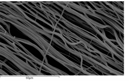
1.2 A SAM image of a polyurethane nanofiber . . . 14
1.3 Dynamic System general representation . . . 15
1.4 System identification flowchart . . . 16
1.5 Nonlinear system discrete-time representation . . . 18
1.6 On the left the serial-parallel model for prediction. On the right side the parallel mode for simulation . . . 19
1.7 Error function for model estimation . . . 20
1.8 Optimization techniques classification . . . 21
1.9 Schematic representation of a perceptron . . . 23
1.10 A general one hidden layer network . . . 23
2.1 Measurement set-up for the electromechanical characterization of the soft actua-tor: the Instron™ ElectroPuls E1000 receives voltages as inputs and registers the response of the specimen (either a force or a displacement). The Instron™ wave-matrix software collects the generated data. . . 25
2.2 Bundle preparation for displacement and force test . . . 27
2.3 Matlab neuron representation . . . 28
2.4 Matlab system identification toolbox interface . . . 29
3.1 Different input Voltage signals. . . 31
3.2 Input/output sampled data. Force test. . . 32
3.3 Matlab neural network representation. . . 34
3.4 Input voltage signals . . . 35
3.5 Sampled output displacement. Displacement test . . . 36
4.1 Training error of forward neural network . . . 38
4.2 Error of closed loop neural network . . . 38
4.3 Comparison real output and neural network output . . . 39
4.4 Comparison outputs of the linear system, neural network and real system . . . . 39
4.5 Training error of displacement test . . . 40
4.6 Validation error. Displacement test . . . 41
7.1 Comparison reference and outputs . . . 51
7.2 Comparison control actions . . . 52
7.3 Arm setup . . . 53
Motivation
Polyurethane (PU) is a versatile thermoplastic polymer. PU has a good mechanical property such as flexibility and low density. The PU is also bio-compatible and is biodegradable, so is easily suitable for medical materials, for example for drug delivery [3].
Polyurethane has been used as a soft actuator. In [9] the bending characteristics of a polyurethane elastomer film with different metal electrodes have been analyzed; Iron chloride has been elec-trospun with a polyurethane matrix in [12] to realize a conductive nanofibrous actuator, while in [1] carbon powders have been used as conductive filler in a polyurethane film to realize MEMS actuators. As pointed out, for example, in [11], controlling soft robots requires new approaches to modelling, control, dynamics, and high-level planning. Known robotics techniques for kine-matic and dynamic modelling cannot be directly used in soft robotics; soft robots are highly nonlinear systems and the sensitivity of the materials can easily cause a change in the dynamics of the system. Several approaches can be found in literature to realize a control model for soft robots: in [15] or in [6] a FEM methodology is used to get a dynamical model of the soft robots, in [16] six different control approaches inspired by classical control theory, machine learning, and neuroscience were evaluated in controlling a cable-driven robot. The nonlinear system iden-tification theory, proposed in this work, could be useful when the physics of the system is too complex to be described just by physical insight; black-box modelling is a good approach for soft robotics, where the different physical effect is the reason of movement of actuators. This paper focuses on a soft actuator realized as a bundle of aligned nanofibers of polyurethane and salt that acts as conductive filling, lowering the electrical resistance of the material. In fact, the driving characteristics of the actuator are influenced by phenomena related to the flowing of current in the material [12]. The nanofibers have been realized through the electrospinning process. Electrospinning is an efficient technique to produce small-diameter (from nanometer to micrometre scale) polymer fibers oriented in the fiber length direction. Nanofibers are charac-terized by high porosity and high surface-volume-ratio and physicochemical properties change is expected to affect the actuation driving process. As claimed in [2] clever usage of materials with reconfigurable, adaptive, and/or tunable physicochemical properties will be a key enabler in the field of soft robotics. Moreover, electrospinning allows producing a soft, biocompatible and lightweight material.
This thesis proposes an electromechanical characterization set-up for the evaluation of force and displacement of a nanofibrous polyurethane-based soft actuator and to realize a model with the experimental data through the nonlinear system identification theory using an MLP neural network to identify the link between the electrical input voltage and mechanical output of the actuator. The obtained model has been used to perform a control system for the soft actuator, and a robotic arm application is proposed. Moreover the performance of the bundle, in term of comparison between electrical power dissipated and mechanical power produced, has been analyzed and compared to the performance of a DC linear motor. From the comparison, is clear the better performance of the bundle in terms of weight and power consumption.
The work is organized as follows: first section Application aims to identify the nonlinear model of the polyurethane-based soft actuator. The second part, Application makes uses of the nonlinear model identified to build a position control law. The second part ends with a possible future application of the soft actuator and energy analysis is presented.
ACTUATOR
This section focuses on the background used for the electromechanical tests and on nonlinear system identification. It is shown how a polyurethane-based soft actuator is produced. Then a model identification for the nonlinear system is explained passing through optimization theory for the neural network application. This section ends with the application nonlinear system identification theory using neural networks, showing the results obtained in two study cases.
Literature
1.1
Electrospinning
Electrospinning is a fiber spinning technique able to produce fibers of nanometric diameter starting from a polymeric solution. This process is possible thanks to high potential voltage that allow the fiber stretching. The general setup for the electrospinning includes a high voltage power supply, a spinneret, a grounded collected plate, and a syringe. The polymer solution is contained inside the syringe, pulled by electronic control. This movement pushes the solution thought the spinneret. Since the spinneret is connected to high potential voltage and the plates grounded, the solution starts to be stretched from the spinneret to the plate. This procedure allows the creation of nanofibers on the plate. Figure 1.1 shows how the electrospinning works. There are other types of setup configuration for other types of fiber production. The one used for the production of the bundle tested in this thesis is the one that uses instead of plates a rolling cylinder. As well as the plate, also the rolling cylinder is grounded. While in the case of the plates the fibers were deposited randomly, with the cylinder, rotating at high velocity, the fibers are aligned.
As said, the process of electrospinning is conducted under a high voltage. This high voltage produces a high electric field. The solution, pushed by the syringe through the pipe, it arrives at spinneret as a drop. When the magnitude of the electric field increase, the drop modifies its shape. Changing the shape, the droplet becomes a jet of solution. When this happens, on the spinneret, it creates a cone shape defined as Taylor cone. The jet created “flies” to the grounded cylinder: the solvents, added into the solution, evaporate when in contact with the air. This gives a pure polymeric filament. [10]
1.2
System Identification
This section provides some background on the theory of the system identification (SI) field. It describes how to identify a system focusing on the nonlinear system identification since the
Figure 1.1: General setup for electrospinning process
physical system studied presents some nonlinear behaviour. A way to identify nonlinear system can be the one using the theory of the neural network. Together with neural network theory, it is exposed also the optimization field with the focus on the gradient-based algorithm used for neural network training.
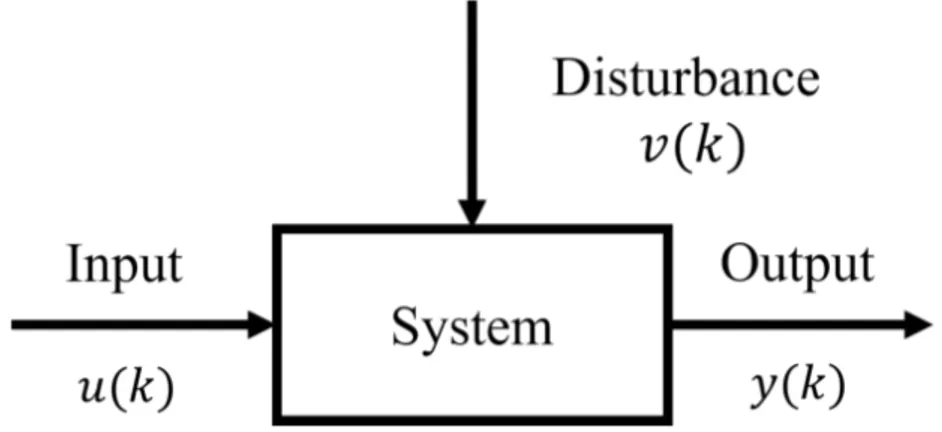
System identification field aims to understand and find a mathematical dynamical model for the physical system. A scheme of a general dynamic system is shown in figure 1.3 From
Figure 1.3: Dynamic System general representation
the figure is possible to notice that the system is driven by an input u(k), and affected by a disturbance v(k). The output is the system dynamic response to a certain input and a certain disturbance. In general for a dynamic system, the control action applied at time k affects the output at time s > k. A model of a physical system is useful on the engineering point of view: a model can be used to analyse the system, to obtain more information useful to predict or simulate the system behaviour. Furthermore, a model can be used to design a good control law. The way to a model of the physical phenomena can be of two types:
• Mathematical modeling. This approach is based on the idea to describe the dynamics of the system using the known laws from physics. This is an analytic approach.
• System identification. This method is based on the data. It starts injecting in the system some known input and sampling the output. This method aims to find the right value of the system parameters such that the data are consistent.
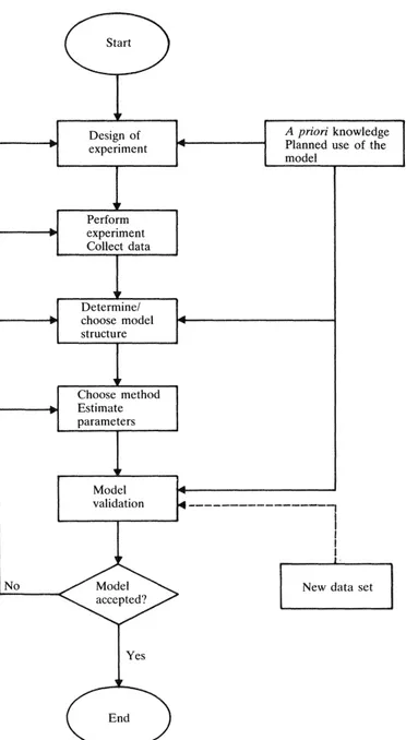
The system identification method is preferred when the physics of the system is too complex to be described just by physical insight. Respect to the mathematical modelling, the SI presents a limited validity. It can be applied only in certain working points and under certain assumptions. Figure 1.4 shows a system identification procedure. It starts with the definition of the prob-lem to be identified. Then the input used to excite the system is sampled together with the response of the system. Once the data has been collected, it is important to choose a suitable model structure. Then it follows the estimation of the unknown parameters of the model. To check if the estimated model is a good representation of the real one, a test is performed. The test is defined in the scheme in Figure 1.4 as a validation step, where if the found model doesn’t
respect the constraints defined, a new identification model has to be used, and the flowchart starts again.
When the model of the system has to be chosen, it is a good practice to stat with the identifi-cation through a linear model. Then if this one doesn’t satisfy the constraint and the behaviour expected, it means that inside that physical system are some nonlinear dynamics. Switching to the nonlinear model, sometimes doesn’t mean better performance: if the system is not chosen enough flexible, it could be even worst then the linear one.
Based on the prior knowledge and the physic insight one can distinguish between three dif-ferent types of model approach [13]:
• White-box models.This case occurs when all the dynamics of the process are well known, and it is possible to describe the dynamics with a mathematical model.
• Grey-box models. This case occurs when some physical insight is known but some pa-rameters have to be estimated from experimental data.
• Black-box models. This case occurs when there is not physical insight, so both the model and the parameters are determinate on experimental data.
The grey-box model advantages and drawbacks are in between the white and black box, giving a good compromise between the two parts.
1.2.1
Nonlinear black-box identification
Let the general discrete-time input/output model, defined as autoregressive exogenous input (ARX) model be:
ˆ
y(k) = b1u(k− 1) + . . . + bmu(k− m) − a1y(k− 1) − . . . − amy(k− m) (1.1)
where bi and ai are scalar parameters, with i = 1 · · · m, ˆy(k) is the estimated output and u(k − m) and y(k − m) are the delayed input and output. It is possible to extend the same
approach to the nonlinear case, obtaining the NARX (nonlinear ARX) where instead of the linear relation ( 1.1) , input and output delays are connected by a unknown nonlinear function
f (·) :
ˆ
y(k) = f (u(k− 1), . . . , u(k − m), y(k − 1), . . . , y(k − m)) (1.2) The concept of estimate the parameters ai and bi are extend to the accurate estimation of the
function f (·). The family of model that describe the link of input and output is define external
dynamics. There is also the so call internal dynamics approach that describes a system using
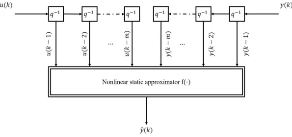
the discrete state space equation approach. In this thesis the external dynamics approach has been used. As shown in Figure 1.5, the nonlinear model can be split into two parts: a nonlinear static approximation and an external dynamic filter, from here the name external dynamics. In
Figure 1.5: Nonlinear system discrete-time representation
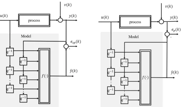
general, the filter is chosen as simple delay q−1. Moreover, the collection of more than one delay is defined as tapped-delay lines. The function f (·) can be chosen among different types, but in this work, the f (·) as been selected to be a neural network. A neural network is suitable for the purpose of this thesis since they can be used for the approximation of a nonlinear function [7]. As defined in the system identification section, a model prediction can be suitable for different purposes. In the case of the dynamic model, it can be used in two configurations, for prediction and simulation. The first one is suitable, as the name says for prediction, meaning that having the process input u(k − i) and process output y(k − i) the model provides the prediction of the output in several steps ahead. On the other hand, in the simulation approach the prediction is based only on the input u(k − i) and the output predicted by the model. From [7], one can distinguish between serial-parallel referring to the one-step prediction configuration, and parallel mode for the simulation configuration. Figure 1.6 shows how the two configurations differ one to the others. The simulation configuration instead is suitable for scenarios where the output cannot be directly measured or also for fault detection. Other difference between the two approaches is the training mode. Both the models are trained by the minimization of a loss function dependent by the error e(k). While in serial-parallel approach the error esp(k)is
called equation error, in the parallel mode the error ep(k) is define as output error. Therefore,
if a second-order model is considered, the predicted output for the one-step prediction model would be:
ˆ
y(k) = f (u(k− 1), u(k − 2), y(k − 1), y(k − 2)), (1.3) while the output simulated by the parallel model would be:
ˆ
y(k) = f (u(k− 1), u(k − 2), ˆy(k − 1), ˆy(k − 2)). (1.4) In this work, the focus is, as said at the beginning of this section, on the external dynamics, one-step prediction, meanly selecting as nonlinear static approximation function f (·) a particular
Figure 1.6: On the left the serial-parallel model for prediction. On the right side the parallel mode for simulation
structure of a neural network: Multilayer Perceptron (MLP) network.
1.3
Optimization
The concept of optimization yield to the idea of minimize (or maximize ) some function. A general optimization problem is defined as [4]:
minimize f0(x)
subject to fi(x)≤ bi, i = 1, ..., m.
(1.5)
where the x is a vector with x ∈ Rn defined as the problem variable. The f0 is defined
as the objective cost function to be minimized, with the domain f0 : Rn → R. Then the
fi : Rn → R i = 1, ..., m are the constraint functions and the vector b collecting all the bi, i = 1, ..., m are the bound of the constraints. The aim of this optimization problem is to find
a vector x∗that is the minimum under ficonstraints respect to the cost function.There exist four
cases of optimal solution:
• x∗ is a global minimum of f0 if f (x∗)≤ f(x) ∀x ∈ Rn
• x∗ is a strict global minimum of f0 if f (x∗) < f (x) ∀x ̸= x∗
• x∗ is a local minimum of f0if Bε(x∗) ={x ∈ Rn| ∥x − x∗∥ < ε}
∀ x, y ∈ Rnand∀ α, β ∈ R (1.6)
When the cost function is nonlinear then the problem became a nonlinear program. In this thesis, data fitting is used. Indeed the aim of data fitting is to find the best model, among the available ones. In this case, the cost function can be assumed as the mismatch error between the observed data and the values predicted by the model. The constraint can be represented by the priory knowledge about the parameters system.
Figure 1.7: Error function for model estimation
Figure 1.7 represents how a cost function can be used: a model f (·) links the input vector to the output. The model is parameterized respect the vector θ such that y = f (u, θ). The aim of the optimization is to find the best approximation of by respect the real one y. The only way to have a better approximation is to tune the parameter θ such the error e(i) is the minimum possible.
The work to reduce the errors and, therefore, to tune the parameter vector θ is associated with the algorithm chosen. Considering the problem (1.6), the optimal solution will be found applying the general algorithm :
xt+1 = xt+ αtdt t = 0, 1, . . .
where αt> 0 , (αt ∈ R)
and dtsuch that if ∇f(xt)̸=, ∇f(xt)dt < 0
(1.7)
The two variables αt and dt are respectively the step size and the direction of the algorithm. Based on the choice of these parameters it is possible to get different converging algorithm. A general procedure to start an algorithm is:
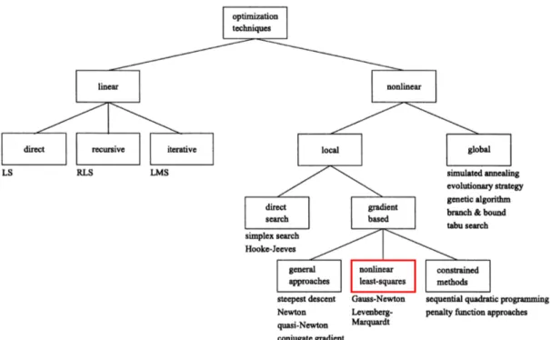
Figure 1.8: Optimization techniques classification 2 select the step size αt.
Figure 1.8 well describes the different level of the converging algorithm: the first layer is composed of different types of cost function. It follows, in the branch of the nonlinear block, the classification based on the type of minimum. Next, considering the gradient base block, it presents three different choices. As highlighted from the figure, in this thesis has been used the nonlinear least-squares Levenberg-Marquardt optimization technique for neural network training. Before to describe the Levenberg-Marquardt, it is necessary to define the meaning of the nonlinear least square. As the name said, this methods is an extension of the classic least square (LS). The nonlinear LS has the advantage to be used with much larger and more general class of functions. The estimation of the parameters is conceptually the same as is in the linear LS. Equation (1.8) defines a general nonlinear LS problem with nonlinear parameters.
f (x) = m
∑
i=1
fi(x)2 (1.8)
with fiare a twice differentiable function. Next, the gradient and the Hessian of f at x can be
computed: ∇f(x) = m ∑ i=1 fi(x)∇fi(x), ∇2f (x) = m ∑ i=1 ( fi(x)∇fi(x)T + fi(x)∇2fi(x) ) (1.9)
J =∇f(x), H =∇2f (x)≈ JTJ (1.10) Coming back to the descent algorithm(1.7), as said, it needs the selection of the direction dt. Selecting an direction of this type :
d =(J JT + βI)−1JTf (1.11) a Levenberg-Marquardt is obtained. The iterative algorithm became:
xt+1 = xt+ αt (
Jt(Jt)T + βtIt
)−1
(Jt)Tft (1.12) The Levenberg-Marquardt is basically an extension of Gauss-Newton algorithm. Starting from Levenberg-Marquardt is possible to approximate the Gauss-Newton algorithm using small value of βt. Setting large value of βtthe algorithm behaves like steepest descent.
This algorithm has been used to train the neural network in the experimental chapter.
1.4
Neural Networks
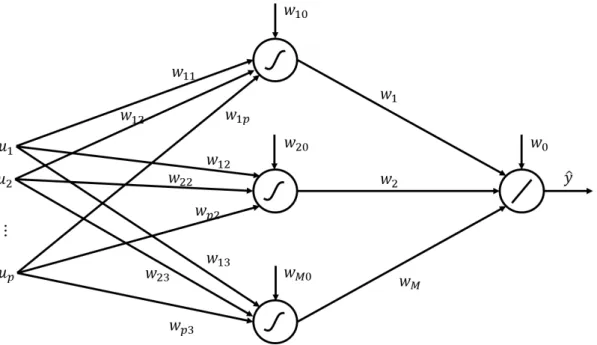
An artificial neural network, in general, is composed of a basic unit defined as neuron. The name neural comes from the inspiration to the human and animal brain [7]. Based on this idea it has been translated and build something similar in mathematical terms. Even if the difference between the real neuron and the artificial one is slightly different, the general idea is similar. Indeed the two neurons had in common some characteristics: a large number of simple units, highly parallel units, strongly connected units, fault-tolerant concerning the failure of a single unit, learning from data. A neural network can have a ridge construction, radial construction or tensor product construction. In this work, it has been considered the rigid construction. Among these categories, the widely known one is the multilayer perceptron network . The basic unit of an MLP is the perceptron. It is composed, as shown in Figure 1.9, by two-part. The first part is composed of the union of the weighted input vector elements. The second part takes the result of the first part, and it projects them though a nonlinear function g(x) obtaining the perceptron output. There are different classes of nonlinear functions, all are saturation function. The func-tion can be sigmoid, logistic, and hyperbolic tangent. To obtain one hidden layer network it is needed the same input on M parallel perceptrons (figure 1.10). The output is the combination of the perceptron outputs and can be computed considering:
Figure 1.9: Schematic representation of a perceptron
Figure 1.10: A general one hidden layer network
ˆ y = M ∑ i=0 wiΦi ( p ∑ j=0 wijuj ) with Φ0(·) = 1 and u0 = 1 (1.13)
where wi are the output layer weights and wij are the hidden layer weights.
An MLP network can approximate any smooth function. More perceptrons are added more the accuracy increases. In general, an MLP network is characterized by two types of param-eters: output layer weight and the hidden layer weight. The first parameters are linear and they establish the amplitudes and the basis function at the operating point. The second, instead, are nonlinear parameters and they define the direction, the slop and the positions of the basis functions. To approximate any smooth function, these parameters have to be tuned. A way to tune them is optimality. The backpropagation is the optimization algorithm used to tune those parameters. Backpropagation is a method for gradients computation on an MPL network. Con-sidering an MLP network with M hidden layer weight, then the derivatives of the MLP output
∂ ˆy ∂wij
= wi dg(x)
dx uj with u0 = 1 , i = 1, . . . , M and j = 1, . . . , p (1.15)
for every weight from the jth input and the ith hidden neuron. The name backpropagation come because the gradient expression is constructed by propagating the model error back through the network. The main algorithms to apply the backpropagation are:
• Regulated activation weight neural network (RAWN), • Nonlinear optimization of the MLP,
• Staggered training of the MLP.
Setup and methods
2.1
Setup
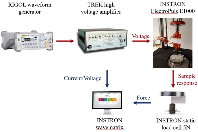
The electromechanical characterization has been performed with the test instrument Instron™ Elec-troPuls E1000 (www.instron.us), equipped with the Instron™ static load cell 2530-5N, which has a capacity of±5 N and a sensitivity of 1.6 mV/V to 2.4 mV/V at static rating. The measure-ment set-up is depicted in Figure 2.1.
Figure 2.1: Measurement set-up for the electromechanical characterization of the soft actuator: the Instron™ ElectroPuls E1000 receives voltages as inputs and registers the response of the specimen (either a force or a displacement). The Instron™ wavematrix software collects the generated data.
The test instrument Instron™ ElectroPuls E1000 is either controlled to maintain a fixed displacement (the extremities of the bundles are kept at a constant distance) to measure the axial contraction force, or to maintain a fixed force to measure the axial displacement. The data are collected at 1 [KHz], by using two strain channels connected to the Instron™ ElectroPuls E1000, and analyzed in a desktop PC through the Instron™ Wavematrix Software. The two strain channels are used to record the displacement or the force, the voltage, and the current that flows through the specimen when the voltage is applied.
2.2
Bundle setting up
The beginning of each experiment, either the displacement of the force test, starts with the se-lection of the bundle to be tested. In this work, it has been selected the polyurethane nanofiber mixed with TABF1salt in a concentration of 10%. The PU its self is a non-conductive material. When the solution is prepared for the electrospinning, together with the PU is added salt in a concentration of 10%. The nanofiber created is still not entirely conductive, due to the only 10% of conductive material. To overcome this problem the nanofiber is soaked in a solvent: the polycarbonate (PC). The soaked mixed nanofiber obtained is a conductive bundle.
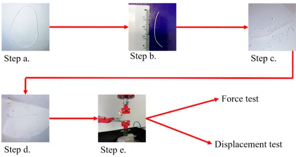
The procedure before to start each test is shown in Figure 2.2. The procedure is divided into different steps. The bundle arrives in a ring shape, Figure 2.2 step (a). Next, a piece of this ring is taken. It has been cut a slice of length 40 [mm] step (b). Then is weighted and the section is measured, resumed in the table 2.1. Once all the dimension of the bundle is measured, the soaking procedure is performed Figure 2.2 step (c).
It has been fixed time of soaking of 30 [s]. This is the time needed for the PC to reach all the nanofibers into the bundle. Immediately after the soaking step, the bundle is dried in a filter paper (step (d)). This step is fundamental otherwise the salt swells out the nanofibers.
Step (e), in Figure 2.2 defines the last procedure before the beginning of the test: the bundle is fixed in both the sides by two conductive clamps. The clamps, internally covered of copper
1tetrabutylammonium
LENGTH 40 mm SECTION 0.6 mm WEIGHT 0.007 g Table 2.1: Dimension bundle
Figure 2.2: Bundle preparation for displacement and force test tape, to apply a voltage at extremities of the bundle.
The clamps together with the bundle are then mounted to the Instron machine: one clamp is attached to the fixed part of the Instron machine (upper part), while the other one is linked to the load cell (down part). At this point using the manual control of the Instron machine, the bundle has been set under a preload of 0.2 [N ]. Due to the pretension, the bundle was straight in the vertical direction. Before the beginning of the test, it has been noticed a negative drift in the preload measured by the load cell. This was due to the internal relaxation of the nanofibers. To have a stable measurement of the force by the load cell, it has been decided to wait for 10 minutes before the beginning of each test. After the last step, one of the two tests has been performed.
2.3
Matlab Neural Network toolbox
Matlab [8] illustrates a workflow for neural network design. First of all, collect the data of the system to analyze. In general, this procedure occurs outside of the NN toolbox software. Next, it must be created the network, under certain choices that will discuss later. After the creation, the network is configured with the proper parameters: numbers of input delays, numbers of hidden layers and numbers of neurons are selected according to the experiment. It follows the initial training of the network. At the end of the procedure is performed a validation using part of the data collected as a tester. There are four types of access to the NN toolbox. Among those, in this thesis it has been used the “command-line” approach, using a Matlab script.
Matlab neuron representation. Important is the function f (·) defined as transfer function. It
Figure 2.3: Matlab neuron representation
can assume different type of function. Moreover the function f (·) produces the (scalar in this case) output a. An important property of the neurons is that can either w and b can be adjustable such that a particular behaviour is obtained by the entire neural network. The idea of the scalar neuron can be extended the usage of vector input (dimension Rx1). The formula 2.2 define the case of the vector as input.
a = f (Wp + b) (2.2)
This time, respect to the scalar case, the weight is not anymore scalar but is a matrix. Indeed the vector p is then post-multiply by the W. As in the scalar case, also in this case a bias b (scalar) is added. If more then one neurons are taken such that each neuron has the same input vector then a One layer of Neurons is obtained. The lantern is composed of the same vector of input but, differently from one single neuron, the output and the bias are vectors. Adding more then
One layer of Neurons in cascade, meaning that the output vector of one layer is the input of the
next one, gives the composition of Multilayers of Neurons. Each layer is characterized by its weight matrix and bias vector. The NN toolbox gives the possibility to choose the structure of the network, in particular, one can choose between two types of input vectors: concurrently and
sequentially. The first is the simplest case of network: it presents no delay in the input and no
feedback. Moreover, the order of the elements of the input vector doesn’t matter. The dynamic case, instead, contains delay and the input vector is a sequence with a certain time order. The NN toolbox allows selecting between two modalities of training: incremental and bash. In the first case, the gradient and the weight computed are updated after each input is applied to the network.
In the bash mode, all the input are applied to the network before the weights are updated.
2.4
Matlab System Identification Toolbox
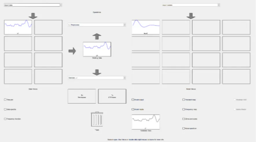
Among Matlab toolboxes, it has been used in this thesis also the system Identification toolbox. From [14], System Identification Toolbox provides MATLAB functions, Simulink blocks, and an app for constructing mathematical models of dynamic systems from measured input-output. It is possible to identify the system dynamics of a complex system using only the data sampled. The input-output data can be either time-domain or frequency-domain to identify continuous-time or discrete-continuous-time transfer function, process model and state-space model. Figure 2.4 shows the user interface of the toolbox. On the left side, there is the location for the input-output
Figure 2.4: Matlab system identification toolbox interface
data upload. Once the data are uploaded, it is possible to perform some pre-processing step i.e.
Remove mean, Remove trends, Resample , and Filter. There are different type of identification:
from the linear one through transfer function, passing from the nonlinear with the NARX model. Depending on the type of system identification, there are some parameters to be chosen. In the case of transfer function the parameters to be selected are the numbers of pole and zero. Once all the settings are ready the estimation of the parameter is performed. The identified function appears in the windows on the right of the user interface (Figure 2.4). From this user interface is possible to compare the real output with the estimated transfer function output. When the model estimated satisfies the requirement of the user, it can be exported to the Matlab workspace
In the experiment chapter, it has been applied the theory of the nonlinear system identification using the neural networks. Specifically, it has been identified the model of the PU plus salt as an actuator. The test performed is divided into two parts: in the first part the bundle is clamped to the Instron machine and the data of voltage and force are sampled. The second part instead aims to control the force applied to the bundle and sample voltage and displacement.
3.1
Force sampling, displacement control
The force test aims to understand the PU plus salt behaviour under a certain applied voltage. The experiment starts applying a preload to the bundle of 0.2 [N ]. Then the idea was to perform a displacement control, such that the distance between the two clamps was constant in time. The Instron machine was in charge to hold the gauge distance. While this control was performed, the load cell was sampling the force provided by the bundle under a certain voltage.
It has been decided to perform three different signal input test: • Two squares input of voltage of 100 and 200 [V ] figure 3.1a ; • A trapezoidal shape with pick of 300 [V ] figure 3.1b;
• A sine wave of period 30 [s] bias 125 [V ], amplitude 250 [V ] figure 3.1c.
The signals just mentioned were obtained through the wave generator RIGOL DG1022, in com-bination with the amplifier. Indeed, as defined by Figure 2.1 , the wave generator gave a signal in mV raised to V by the amplifier TREK MODEL 10/10B-HS.
After the windows of 10 minutes for cell load stabilization, the force measured has been reset to zero. Then the first test has been performed. The Instron machine allows sampling concurrently both the force on the load cell and the voltage applied to the bundle. The two signals have been sampled at the frequency of 1 [kHz]. Once the three tests have been performed, the Instron machine has been saved the sampled data in .CSV format. The data have been then processed and saved in an excel file. The latter file has been composed of two-column cells for
(a) Squares input (b) Trapezoidal input
(c) Sine input
(a) Squares output (b) Trapezoidal output
(c) Sine output
Figure 3.2: Input/output sampled data. Force test.
Having the sampled data the identification part has been executed. To perform a system identification, it has been created a Matlab code defined in the following:
• MAIN.m the script, the core of the code identification;
• Import_data.m responsible for the upload of the sampled data from the excel file to the
Matlab work-space;
• NN_narx_exe_V_F.m with the aim to initialize and perform the neural network identifi-cation.
When the MAIN.m is launched, the sampled data of input-output of each of the three signals are upload in vectors using the script Import_data.m. In the same script has to be define the input
Type NN NARX feedforward-closed loop
# HIDDEN LAYERS 1
# OUTPUT LAYERS 1
# INPUT DELAYS 6 for y ; 6 for u
# NEURONS HIDDEN 10
MINIMUM GRADIENT 1e− 11
TRAINING METHOD trainlm ( Levenberg–Marquardt)
FUN. HIDDEN LAYER sigmoid
FUN. OUTPUT LAYER linear
Table 3.1: Setting for neural network
vectors for the training part and those for the validation part. Moreover, the number of delay
input and output, and the number of neurons for the neural network have to be specified. The NN_narx_exe_V_F.m script is contained in the MAIN.m and aims to set up the neural network and
start the training with the sampled data. Table 3.1 shows the main features of the NN adopted. The script starts with the creation of a feedforward “NARX” net with one hidden layer composed by 10 neurons. The function used by the neurons to link the combination of the inputs, with the output of the hidden layer is a sigmoid function. The output of the sigmoid is then combined in a linear function to get the neural network predicted output. The NN created is shown in figure 3.3a. In the script NN_narx_exe_V_F.m has to be defined the setting of the minimum gradient limit within which the training process stops. If the training procedure doesn’t reach the minimum gradient within the number of “epochs” defined, the training procedure will stop. By default, the training method is assumed as trainlm ( Levenberg–Marquardt). Once all the settings have been set, the training command has been performed. When the NN has to be trained, it needs both the input and the output of the sampled data, that in force test are voltage and force. This configuration is called open-loop or feedforward network (figure 3.3a). When, instead, the output (force) has to be predicted starting from a known input (Voltage), a closed-loop NN has to be used. Closed-closed-loop NN means an open-closed-loop NN where the output predicted is used as feedback input. Figure 3.3b well illustrates a closed-loop NN. With the creation of the closed-loop NN, the script file NN_narx_exe_V_F.m finishes its job. Then is the MAIN.m that provides the command to extract a Simulink block from the closed-loop NN.
The usage of nonlinear system identification in these experiments comes from the behaviour of the bundle. It has been decided to perform also a linear identification of the model. The linear model was discharged because the nonlinear identification with the neural network just fit better the real data. To demonstrate what just claimed, a linear system identification has been performed using the Matlab toolbox System Identification. As defined in the method chapter, the toolbox presents the interface to, first upload the data, and then to use different modalities to identify the system. To be consistent, the same input data of the nonlinear identification has been used (Figure 3.2). It has been performed the linear identification through the transfer function
(a) Forward neural network
(b) Closed loop neural network
Figure 3.3: Matlab neural network representation.
parameters estimation. The best combination of number of pole and zero has been a transfer function with 7 poles and 5 zeros.
The transfer function has been:
T (s) =
−1.497−09s5− 4.515−12s4+ 9.188−14s3+ 9.97−16s2− 8.963−20s + 7.637−23
s7+ 1.56−2s6+ 3.25−4s5 + 4.19−06s4+ 1.556−08s3+ 1.349−11s2+ 1.509−15s + 1.271−18
(3.1)
3.2
Displacement sampling, force control
The experiment for the displacement test aims to understand how the PU plus salt behaves under certain voltage signal. This time is examined the displacement of the bundle applying on the two sides of the bundle a constant preload of 0.2 [N ]. Doing this test it has been defined the relation between the input voltage [V ] and the output in displacement [µm]. Different from the force test, in this test the Instron machine has performed a control on the force applied to the bundle. While the previews test was just asked to hold constant in time the gauge distance, in this test the Instron machine was performing a PID control of the force, holding it constant to 0.2 [N ]. As well as the previous test, also in the displacement test have been used three inputs though the wave generator:
• two squares shapes of 100 and 200 [V ] ; • a trapezoidal shape of peck of 200 [V ] ;
Figure 3.4 shows the input and the output sampled in the displacement test.
(a) Squares input (b) Trapezoidal input
(c) Sine input
Figure 3.4: Input voltage signals
As defined in the Bundle set up, it has waited for 10 minutes for the cell stabilization. The preload of 0.2 [N ], it has been applied with a ramp of 10 seconds and then the experiment has been started. With a sampling frequency of 1 [kHz] both the input (voltage) and output (displacement ) have been sampled. In Figure 3.5 are shown the output displacement responses of respectively squares, trapezoidal and sine shape.
Once the sampling test has been finished, the identification part started. The idea of the identification is basically the same of the force test, but with some changes in the NN setting. As the input of the NN has been used the collection of the inputs and outputs sampled.
(a) Squares output (b) Trapezoidal output
(c) Sine output
Figure 3.5: Sampled output displacement. Displacement test
Type of NN NARX feedforward-closed loop
# HIDDEN LAYERS 1
# OUTPUT LAYERS 1
# INPUT DELAYS 3 for y ; 3 for u
# NEURONS HIDDEN 10
MINIMUM GRADIENT 1e− 11
TRAINING METHOD trainlm ( Levenberg–Marquardt)
FUN. HIDDEN LAYER sigmoid
FUN. OUTPUT LAYER linear
Results
In this chapter, it will be analyzed the results coming from the experimental part. The results are divided into two parts following the division done in the experimental part: Force test results and Displacement test results.
4.1
Force test result
The train of the neural network, in general, didn’t stop because the minimum gradient was reached but cause the number of epochs was reached. This implies that the minimum gradi-ent was too low. In performing the training of the open-loop NN, has been computed the error between the sampled force data and the predicted one. Figure 4.1 shows the error in open loop. As was possible to see, the error was low enough to say that the trained NN was a good ap-proximation of the real system. To define the validity of the NN in the closed-loop has been furnished as input only the signal in Figure 3.1c. What has been obtained is shown in Figure 4.3. Figure 4.2, instead, shows the error between the NN output respect the sampled force. To have a double-check of the goodness of the nonlinear model identified, the same input has been used in the linear model. Figure 4.4 shows the response of the two systems. Is easy to see that the nonlinear model better fit the real output. Moreover, to have a comparison between the two methods of identification, it has been computed the Root Mean Square Error of the two identi-fications. The value computed confirms the goodness of the nonlinear model respect the linear one, indeed:
RM SE(eN N) 0.0014 RM SE(el) 0.0030
Table 4.1: Root Mean Square Error for identification error
Figure 4.1: Training error of forward neural network
Figure 4.3: Comparison real output and neural network output
the figure is possible to notice how the training error is low enough to say that the NN is a good approximation of the training data. To validate the NN it has been selected one of the input signals, the one shown in Figure 3.5c. Figure 4.7, shows the comparison of the sampled displacement data and the NN output prediction. During the training phase have been used a different combination of input delays and a different number of neurons but the best combination has been the one shown in the table 3.2. Finally has been analyzed the error between the real output and the estimated one. Figure 4.6 shows the comparison error. As in the case of the force test, the Root Mean Square has been computed on the comparison error. It comes out an
RMSE of 0.0044. It has been performed also a linear identification of the system based on the
same training data of the NN. The one step ahead prediction of the linear model was completely different even trying to change the configuration of poles and zeros.
Figure 4.5: Training error of displacement test
Another point to make is related to the figures 3.5c. It is possible to notice that when the voltage inverts the polarity, the bundle had a contraction in a positive direction. So either the input is positive or negative, the bundle will move always in the same direction with the same intensity. The fact that the strain (S) is always in one direction can be explained by its quadratic dependency to the electric field. The electrostrictive law well defines this behaviour [5]:
Figure 4.6: Validation error. Displacement test
where Q is the charge-related electrostrictive coefficient and P is the polarization or electric field. The electrostriction is not the only phenomena acting on the bundle, indeed as reported by [12], the behaviour of the bundle is due to different phenomena i.e. thermal, electrostrictive, electromechanical, so it is not easy to have a well defined physical model. From this reason come the needed to switch to a nonlinear black-box identification.
APPLICATION
In the first part of this work, it has been analyzed and defined the black-box model for the bundle of PU plus salt. As introduced in the first part the PU plus salt can be seen as an electroactive soft actuator. This second part shows a possible usage of the identified actuator: a position control and energy analysis for application of the bundle as artificial muscles have been found.
Control setup
The setup used for the control part is mostly the same used for the identification part. It has been used a Raspberry pi model B 3 to perform the control unit. The output signal of the Raspberry pi is then amplified by the operational amplifier lm324n. The output is then used to drive a MOS-FET connected to the amplifier TREK MODEL 10/10B-HS thought a BNC cable. It has been used two 3D printed clamps in ABS for the position control, and a 3D printed ABS structure to show a possible application of the bundle. In the position control has been used the Logitech Hd Pro Webcam C920 camera for position tracking. A laptop it has been used for image calibration and for upload the code in the raspberry board.
6.1
Position control
From the first part it has been demonstrated that under a certain applied voltage, the bundle of PU plus salt contracts up to 40 [µm].
(a) PU plus salt property (b) Position control set-up Figure 6.1: Control clamps setup
The setup for the experiment is shown in Figure 6.1b: the bundle is held on one side by a fixed clamp. The other side of the bundle is then held by another clamp free to move. The weight of the free clamp is 17.67 [g]. This implies that on the free side of the bundle is applied a force of 0.17 [N ], similar to the preload defined in the identification section. To build a suitable
control action for the model (voltage-displacement), it has been created a simulation test scheme
( Figure 6.2) in the Simulink environment.
A discrete PID has been selected considering a sample time of 1 [Hz] and the parameters of the proportional KP, integral KI and derivative KD action reported in table 6.1. Once the
control law has been define can be exported to the electronic board Raspberry pi. The Figure 6.3 shows as the Raspberry pi has been used as a control unit for the displacement monitoring and control. Note that the camera Logitech has been connected to the raspberry board for images acquirement. The camera has been used as position tracking to have an indirect access to the
Figure 6.2: Simulation scheme
KP 7000
KI 300
KD 200
Table 6.1: PID control parameters
position of the free clamp. This sensor has been used as a feedback sensor. For the actuation instead has been used a signal conditioning circuit. From the Raspberry pi GPIO 18 has been produced a Pulse-width modulation (PWM) wave ranging from 0 to 3.3 [V ]. This signal is then amplified through an operational amplifier up to 5.5 [V ]. The latter is next used to drive the gate port of MOSFET. From the MOSFET it has been obtained an output voltage of 0− 250 [mV ] then amplified by the TREK MODEL 10/10B-HS up to 0− 250 [V ].
6.1.1
Image calibration for potion control
Before to embed the control in the Raspberry and proceed in the experiment, an offline procedure for image calibration has been done. The procedure can be resumed in four steps:
• acquire the image from the camera; • define the gain P ixel → mm;
• define the reference coordinates (x0, y0);
• define the pixels region of interest.
The first step is the acquisition of the image with the laptop. Figure 6.4a shows Matlab reference axes (0, 0) coordinates defined in the upper-left corner. Step 2 aims to convert a displacement of tracked points in mm. Each time the clamp is removed and put back, the cal-ibration procedure has to be performed again. In defining the region of interest is worth to mention how Matlab define it. In general, the region can be defined in a different method, but the one that has been used is the “imrect”: the region is defined by a 4-element vector of the
Figure 6.3: Raspberry pi setup, control law uploading
form [ xmin ymin width height ]. The first two are x and y coordinates of the upper-left corner
of the rectangle. Then the other two are respectively the width and the height of the rectangle. All the points are defined in pixel. Step 3 has been used to define the new references axes. The parameter obtained from the image calibration are: initial reference, (x_init y_init), the region
of interest, and gainPx2mm.
6.1.2
Control script
The control script has been written in the Matlab language. It has been divided into different parts. The first parts contain all the initialization instructions i.e Raspberry pi configuration (need for the upload of the code from Matlab to the Raspberry), camera initialization (needed to allow Raspberry pi to take a picture from the Logitech Hd Pro Webcam C920). Moreover have been defined also the parameters for the PWM i.e frequency, duty cycling and Raspberry GPIO. Then are insert manually the value of initial reference, (x_init y_init), the region of
interest, and gainPx2mm defined in the offline image calibration step. Next, it has been defined
all the parameters concerning the control part i.e the control parameters (KP , KD, KI ), the
reference and the sample time. Since the PWM function accepts only values within [0 1], it has been defined as a linear mapping function, from the control action to PWM values.
At this point, it has been defined the core of the control part that cycles these instructions: • it acquires a frame image;
• having in memory the region of the points to be tracked, the code gives back the coordi-nates of the points in frame sampled;
• the points obtained, are expressed respect the new reference, and converted in mm; • the error between the reference and the actual position is computed;
(a) Step 1: image acquiring, Matlab image reference (b) Step 2: definition of the gain to convert pixels in mm.
(c) Step 3: definition of the new axes reference
(d) Step 4: definition of the region of interest (e) Step 4: definition of the points of interest Figure 6.4: Offline image calibration procedure
Results
In the first part, the result of the position control has been reported. It follows a possible future application of the PU plus salt as a robotic arm. The chapter finishes with an energy analysis of the bundle of PU plus salt.
7.1
Position control result
This section collects the results obtained from the clamp position control. As explained in the experiment part, the position control has been used to test the identified model of the bundle of PU plus salt. As said, first has been defined as a simulation in Matlab Simulink and then, the controller has been translated in Matlab code for Raspberry pi. It has been decided to control the position of the clamp attached to the bundle, specifically it has been asked to the controller to follow a step reference of 40 [µm] for the duration of 20 [s]. Figure 7.1, shows the comparison
Figure 7.1: Comparison reference and outputs
Figure 7.2: Comparison control actions
of the reference with the output of the experiment and simulation. It is possible to notice how the experimental output and the simulation are not overlapped: this can be explained by the noise due to the camera. Indeed, in the experimental output, the camera is used as a position sensor. To speed up the control action, it has been decided to reduce the resolution of the image acquired for position tracking. Doing so, a noisy position output come out and as consequence also the control action as been affected as shown in Figure 7.2.
7.2
Future application
During the work done, it has been thought a possible application for the polyurethane-based actuator: a robotic arm. Indeed, has been thought to use the actuator as a small artificial muscle adopted to move a small copper-based arm. Figure 7.3 shows the 3D printed structure. It is possible to notice that the copper tape has been added in the fulcrum of the arm. Moreover, the arm itself has been made by copper such that one side of the bundle is connected to the positive pole of the power supply. The other side of the bundle has been connected to the negative pole of the power supply through a copper tape. Tt has been performed a test applying a voltage of 300 [V ] to the two sides of the bundle. While the step input signal it has been applied, a video has been recorded. A the end of the experiments the tracking position has been done. Starting from the video has been taken the first frame and has been performed the same image calibration procedure seen in the Image calibration section. Once the new reference, region of interest, and
gainPx2mm has been defined, a Matlab script has been executed. The procedure has been done
in the same way as the position control but with some modification. First, the image has been acquired from the video, taking one frame per iteration. Then have been identified the points of
(a) Arm setup without bundle (b) Arm setup with bundle Figure 7.3: Arm setup
interest and has been extracted their coordinates. Since the points identified are more than one, it has been formed either for the x coordinate and for y the average among the coordinates of the points. Once the coordinates have been found, the pixel coordinates are expressed respect to the new reference axes. Having the position of the point respect to the axes, it has been computed the angle. Figures 7.4 hows how the angle had changes in time.
Figure 7.4: Arm displacement with 300 V input
7.3
Energy analysis
To show the performance of the bundle, and energy analysis has been performed. In particular, the electric power consumption and the force produced with respect to the weight of the material has been compared with the performance of a DC linear motor (LINMOT PO1-23x80,https: //linmot.com/).
imen. The weight of the free clamp converted in N is comparable to the applied preload in the electromechanical characterization. In this way, it is possible to reasonably use as reference the contraction force values obtained during the electromechanical characterization. The dissipated electric power Pelof the soft actuator is:
Pel = V I (7.2)
For the comparison, it is assumed to realize an actuator with multiple bundles in parallel. The bundles contract in the same direction with the same force and the electric current flowing in the samples is the same for every bundle. It is possible to calculate the amount of total weight Wtotof the PU, which is required to produce the same amount of force generated by the
linear motor with a simple proportion, knowing the force produced by the single bundle (Ftot)
expressed in kg, its weight and the force generated by the motor expressed in kg. If the bundles are connected in parallel, it is possible to calculate the number n of bundles necessary to produce the force generated by the motor, i.e.:
n = Wtot Wbundle
(7.3) where Wbundleis the weight of the single bundle. Moreover the total power consumption is given
by:
Ptotal= nPel (7.4)
The comparison of the energy analysis is summarized in Table 7.1. The values of the current, relatives to the bundle, used for the analysis have been evaluated through the high-voltage am-plifier, and are referred to the maximum applied voltage of the test of position control (250 [V ]), that led to a peak current value of 1.8 [mA].
Weight (g) Adsorbed Power (W) Max Force (kg)
Motor 265 280 4.486
Bundle ∼0.007 ∼0.45 ∼0.0234
Parallel bundles ∼1.34 ∼86 ∼4.486
Table 7.1: Comparison of performance between a DC motor, a single bundle and a parallel connection of several bundles.
This work focuses on the analysis and utilization of an electroactive soft actuator, made of polyurethane-based nanofibers. On a bundle made by aligned nanofibers of polyurethane and a salt has been performed several electromechanical test using the machine Instron™ static Elec-troPlus E1000 equipped with the Instron™ static load cell 2530-5N. The data sampled of volt-age, force, and displacement have been then used for nonlinear system identification of the soft actuator bundle. It has been noticed the quadratic dependency between voltage and displace-ment/force. A possible application of the soft actuator has been designed. To conclude it has been compared the soft actuator with a linear DC motor: it has been shown how a collection of parallel bundles of PU plus salt absorbs less electric energy respect to linear DC motor, based on similar maximum output force. Thanks to the low-cost production, to the better efficiency, to the low weight-bundle/weight-lifted, the polyurethane-based soft actuator could be used to replace electric motors.
[2] Théo Calais and Pablo Valdivia y Alvarado. “Advanced functional materials for soft robotics: tuning physicochemical properties beyond rigidity control”. In: Multifunct. Mater 2 (2019).
[3] Jong Yuh Cherng et al. “Polyurethane-based drug delivery systems”. In: International
Journal of Pharmaceutics 450.1 (2013), pp. 145–162. ISSN: 0378-5173. DOI:https:// doi.org/10.1016/j.ijpharm.2013.04.063. URL: http://www.sciencedirect. com/science/article/pii/S0378517313003645.
[4] Notarstefano Giuseppe. Note of Distributed control system. 2019.
[5] Kwan Chi Kao. Dielectric Phenomena in Solids. Vol. 1. Elsevier Academic Press, 2014, pp. 49–50.
[6] Frederick Largilliere et al. “Real-time Control of Soft-Robots using Asynchronous Finite Element Modeling”. In: ICRA (2015), p. 6.
[7] Oliver Nelles. Nonlinear System Identification, From Classical Approaches to Neural
Networks and Fuzzy Models. Vol. 1. Springer, 2001, pp. 49–50.
[8] Neural Network Toolbox User’s Guide. October 2004.
[9] Ohmukai et al. “Electrode Effects on Polyurethane Soft Actuator”. In: World Journal of
Engineering and Technology 05 (Jan. 2017), pp. 520–525. DOI:10.4236/wjet.2017. 53044.
[10] Seeram Ramakrishna. An Introduction to Electrospinning and Nanofibers. World Scien-tific Publishing, 2005.
[11] Daniela Rus and Michael T. Tolley. “Design, fabrication and control of soft robots”. In:
Nature 521 (2015), pp. 467–475.
[12] Hiroaki Sakamoto et al. “Fabrication and Characterization of FE/Polyurethane Nanofiber Actuator Prepared by Electrospinning”. In: Journal of Fiber Science and Technology 73 (6 2017), pp. 135–138.
[13] Jonas Sjöberg et al. “Nonlinear black-box modeling in system identification: a unified overview”. In: Automatica 31.12 (1995). Trends in System Identification, pp. 1691–1724. ISSN: 0005-1098. DOI:https://doi.org/10.1016/0005-1098(95)00120-8. URL: http://www.sciencedirect.com/science/article/pii/0005109895001208. [14] System Identification Toolbox™ Getting Started Guide. October 2004.
[15] Maxime Thieffry et al. “Dynamic control of soft robots”. In: IFAC World Congress (2017). [16] S. Wittmeier et al. “Toward anthropomimetic robotics: development, simulation, and
The work done has been developed together with R. D’Anniballe and R. Carloni from the Faculty
Fabrication, Modeling, and Control
Giovanni Paoletta1, Riccardo D’Anniballe2, and Raffaella Carloni2
Abstract— This paper presents the analysis and utilization of an electroactive soft actuator, made of polyurethane-based nanofibers. A mat of aligned nanofibers of polyurethane and a salt has been fabricated through an electrospinning process and, subsequently, has been rolled up to form a bundle of aligned nanofibers. From the same bundle, three specimen have been obtained, i.e., three polyurethane-based soft actuators. Several electromechanical tests on one specimen have been performed to evaluate the forces and the displacements generated by the soft actuator when an electrical input is applied. The data generated during the electromechanical tests have been used in a neural network to derive the non-linear model of the soft actuator. Subsequently, the model has been used to design a position control scheme, which has been tested on a second specimen. The performances of the soft actuator have been compared to a DC linear motor with similar maximum output force. Finally, to validate the contraction capabilities of the soft actuator, a third specimen has been used to actuate a robotic arm.
I. INTRODUCTION
Polyurethane (PU) is a versatile thermoplastic polymer with good mechanical property, such as flexibility and low density. PU is also bio-compatible, biodegradable and, there-fore, suitable for medical applications [1]. PU has been also used as soft actuator. In [2], the bending character-istics of a film of a polyurethane elastomer with different metal electrodes has been analized. Iron chloride has been electrospun with a polyurethane matrix in [3] to realize a conductive nanofibrous actuator. In [4], carbon powders have been used as conductive filler in a polyurethane film to realize microelectromechanical actuators.
Soft actuators and soft robots requires new approaches for dynamic modeling and control [5]. Classical kinematic and dynamic modeling techniques cannot be directly used in soft robotics because soft robots are highly non-linear systems, and the sensitivity of the materials used therein can cause a change in the dynamics of the system. Several novel control approaches can be found in the literature: in [6] and [7], finite element methods are use to derive a dynamical model of the soft robots, in [8] different control approaches inspired by classical control theory, machine learning, and neuroscience have been evaluated for the control of a cable-driven robot.
This work was funded by the European Commission’s Horizon 2020 Programme as part of the project MAGNIFY under grant no. 801378.
1Giovanni Paoletta is with the Faculty of Engineering, University of
Bologna, [email protected](This work was done while G. Paoletta was with the Faculty of Science and Engineering, University of Groningen, The Netherlands.)
2R. D’Anniballe and R. Carloni are with the Faculty of
Sci-ence and Engineering, University of Groningen, The Netherlands.
{r.danniballe,r.carloni}@rug.nl
This paper focuses on a soft actuator, which consists of a bundle of aligned nanofibers of polyurethane and a salt that acts as conductive filling. The aligned nanofibers have been realized through an electrospinning process, i.e., an efficient technique to produce small-diameter (from nanometer to micrometer scale) polymeric fibers oriented in the fiber length direction. Nanofibers are characterized by high poros-ity and high surface-volume ratio, and their physicochemical properties can affect their actuation driving process [9].
In this paper, the soft actuator is analyzed and elec-tromechanically characterized to evaluate the forces and the displacements generated when an electric field is applied. The experimental data are used to derive a non-linear dy-namic model, which has been identified by using an artificial neural network. The obtained model has been used to design a position control scheme for the soft actuator and for a robotic arm, in which the soft actuator is implemented. The performances of the soft actuator have been compared to a DC linear motor in terms of dissipated electrical power and produced mechanical power.
The remainder of the paper is organized as follows. Sec-tion II presents the fabricaSec-tion of a PU-based soft actuator. Section III presents the experimental set-up to measure the forces and displacements produced by the soft actuator when an electric field is applied. In Section IV, the dynamic model of the soft actuator is derived by using a non-linear system identification method based on an artificial neural network. In Section V the model is used to design a control system for the position control of the soft actuator. In Section VI a robotic arm that exploits the soft actuator is realized and tested. Finally, concluding remarks are drawn in Section VII.
II. FABRICATION OF THE POLYURETHANE-BASED SOFT ACTUATOR
This Section presents the fabrication of the nanofibrous PU-based soft actuator, as sketched in Figure 1.
The soft actuator consists of a bundle of aligned nanofibers of PU1 and a salt2. The aligned nanofibers have been fabri-cated by an electrospinning process [10], [11], in which the polymeric solution of PU and the salt is stretched in a high electrostatic field. Specifically, the electrospinning machine consists of a syringe with a thin metallic needle, loaded with the solution and a solvent, a syringe pump to control the flow rate, and a metallic rotating collector positioned at a certain distance. The needle is linked to the positive
1
Poly[4,4-methylenebis(phenylisocyanate)-alt-1,4-butanediol/di(propyleneglycol)/polycaprolactone].