Mixing in gravity currents

(1)

Ph.D. IN ENGINEERING CIVIL ENGINEERING SECTION

XXVII CYCLE

Ph.D. Student: Ing. Luisa Ottolenghi

Tutor:

Prof. Claudia Adduce

Coordinator Ph.D. Course: Prof. Aldo Fiori

ﬁrma della tesi esteso...

(2)

Collana delle tesi di Dottorato di Ricerca In Scienze dell’Ingegneria Civile

Universit`a degli Studi Roma Tre Tesi n◦ 52

(3)

A Paolo, because he had the Ocean ﬂowing in his veins

(4)

(5)

He made it to the ocean Had a smoke in a tree

The wind rose up, set him down on his knees A wave came crashing like a fist to the jaw Delivered him wings -”Hey, look at me now” Arms wide open with the sea as his floor ... He’s flying! Oh, high! wide!

(6)

(7)

Abstract

The dynamics of buoyancy-driven flows are investigated focusing on the mix-ing processes occurrmix-ing between the dense current and the surroundmix-ing fluid. This kind of flows widely occurs in the environment, due both to natural and anthropic causes: examples are sea breeze fronts, oceanic overflows, and pollutant discharges in water bodies.

In this study steady and unsteady gravity currents are analysed by means of laboratory experiments and Large Eddy Simulations. Unsteady gravity cur-rents propagating over horizontal and up-sloping boundaries are generated by the lock-exchange technique, and are studied by a combination of labo-ratory experiments and numerical simulations. Steady gravity currents are reproduced experimentally by the release of a constant discharge of dense fluid in a lighter ambient fluid. The gravity current is then allowed to flow down a rough inclined bottom, in a rotating environment.

A total of 12 laboratory experiments and 16 LES of lock-released gravity currents are performed, varying the initial reduced gravity g₀′, the aspect ratio of the initial volume of the dense fluid in the lock R, and the in-clination of the bottom boundary θ. A good agreement is found between the numerical LES results and the experimental measurements. Different phases during the propagation of the dense current are observed: a slump-ing phase followed by a self-similar phase and an eventual viscous phase are detected. The visualization of the three-dimensional density iso-surface shows the presence of two kinds of instability characterizing all the simu-lated cases: Kelvin-Helmholtz billows and lobe-and-cleft structures, and it is found that their development strongly affects mixing.

The increase in velocity of the front of the gravity current is visible with the increase of g₀′ or with a decrease of R. On the contrary, as expected, increas-ing the steepness of the bottom, the dense current slows down. Furthermore, in gravity currents propagating up a slope, the presence of a reversed ﬂow close to the bottom of the domain is clearly visible, which causes an accu-mulation of dense ﬂuid in the lock region of the tank.

(8)

Mixing processes occurring between the dense current and the ambient fluid are analysed according to different approaches: two entrainment pa-rameters are defined (Elocal and Ebulk) and the energy budget method of

Winters et al. [1995] is applied. The analysis shows that a greater amount of mixing is observed as R decreases. In addition, as expected, a decrease of mixing with the increase of the steepness of the bottom is observed. Turbulent quantities are analysed, finding that turbulence is more pro-nounced at the interface between the dense and the ambient fluids, particu-larly in the head region and and in correspondence of the Kelvin-Helmholtz billows, indicating the occurrence of significant mixing in these regions.

The dynamics of steady gravity currents flowing down an incline on a rough bottom boundary in a rotating environment are investigated by labo-ratory experiments, focusing on the effects on mixing of the variations of the roughness and of the inclination of the slope s. A total of 68 experiments are performed and different flow regimes are observed, depending on s and on the density of the roughness λc. During the laminar regime, low values of the entrainment parameter are found. For higher values of s, non-breaking wave regime and breaking-wave regime occur, during which a great amount of ambient fluid is entrained by the gravity current. The higher values of E are observed during the turbulent regime, which is found in presence of high values of s.

In the experiments performed on the same roughness, the increase of E with the increase of s is distinctly detected. The presence of a rough bottom causes the occurrence of two different mechanisms acting oppositely: addi-tional turbulence is generated due to the presence of the roughness, which acts enhancing mixing, but, at the same time, the velocities in the flow de-crease for the presence of the rough elements, and consequently, turbulent structures are inhibited. In general, the presence of a rough bottom acts increasing the entrainment. A good correspondence is observed between the present study and the investigations on flows propagating within aquatic vegetation [Nepf , 2012]. The analysis of the density measures taken at dif-ferent heights during the experiments shows a stratification within the body of the gravity current which is in agreement with the Nepf [2012] classifi-cation: increasing the density of the roughness, the stratification within the body of the dense current becomes more visible, until significant differences in density between the parts of the fluid belonging to the regions inside and outside the roughness are observed for high values of λc.

(9)

List of Figures

2.1 Experimental apparatus for unsteady gravity currents . . . . 15

2.2 Deﬁnition of the near wall regions . . . 24

2.3 Analysis of the grid resolution . . . 26

2.4 Density ﬁeld in a gravity current: iso-density levels . . . 29

2.5 Experimental pictures and numerical density ﬁeld . . . 30

2.6 Density ﬁeld for EXP3 . . . 31

2.7 Density ﬁeld for RUN3 . . . 32

2.8 xf(t): inﬂuence of R and g0′ . . . 34

2.9 x∗_f(T∗): inﬂuence of R . . . . 36

2.10 Front position of gravity currents ﬂowing up a slope . . . 38

2.11 Analysis of ⟨ρ∗⟩ at ﬁxed height . . . 40

2.12 Kelvin-Helmholtz billows in the density ﬁeld . . . 41

2.14 ⟨u⟩ vertical proﬁles for RUN1 . . . 44

2.15 ⟨u⟩ vertical proﬁles for RUN9 . . . 45

2.17 Velocity ﬁelds for diﬀerent θ . . . . 48

2.18 Three-dimensional density ﬁeld for RUN1 . . . 50

2.21 Ebulk and Elocal varying R and g0′ . . . 54

2.22 Trapping of ambient ﬂuid process . . . 56

2.23 E versus Fr and E versus Re for RUN1 ÷ RUN9 . . . 58

2.24 Ebulk and Elocal varying θ . . . . 60

2.25 E versus Fr , E versus Re and E versus s . . . 61

2.26 E versus Fr , present and previous results . . . 63

2.27 Variation in volume of the gravity current: Ai/A0 versus x∗f . 66 2.28 Energy budget method . . . 69

2.29 Energy budget for RUN1÷ RUN9 . . . 70

(12)

2.31 Energy budget varying θ . . . . 75

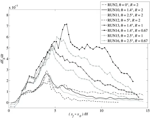
2.32 dEbH/dt versus (xf − x0)/H for the up-sloping cases . . . . . 76

2.33 Dimensionless ﬂuctuating velocity for RUN2 . . . 78

2.36 Turbulent kinetic energy budget . . . 81

2.37 Evolution in time of k . . . . 82

2.38 Evolution in time of B . . . . 83

2.39 Evolution in time of P . . . . 84

2.40 Evolution in time of ε . . . . 85

3.1 Lateral view of the experimental apparatus at WHOI . . . 90

3.2 Top-view of the experimental apparatus at WHOI . . . 95

3.3 Density of the roughness . . . 98

3.4 Diﬀerent ﬂow regimes in steady gravity currents . . . 101

3.5 Diﬀerent ﬂow regimes varying the roughness . . . 103

3.6 E versus Fr varying the roughness of the bed . . . 106

3.7 E versus Re varying the roughness of the bed . . . 107

3.8 E versus Fr varying the slope of the bottom . . . 108

3.9 E versus Fr varying λc and s . . . 110

3.10 E versus Fr varying s and λc . . . 112

3.11 E versus s varying the roughness of the bed . . . 114

3.12 Stratiﬁcation in the gravity current: sparse canopy cases . . . 117

3.13 Stratiﬁcation in the gravity current: intermediate canopy cases119 3.14 Stratiﬁcation in the gravity current: dense canopy cases . . . 120

(13)

List of Tables

2.1 Laboratory experiments performed. . . 14

2.2 Parameters of the laboratory experiments. . . 15

2.3 Numerical simulations performed. . . 21

2.4 Parameters of the numerical simulations. . . 22

2.5 Values of the dimensionless grid spacings. . . 27

3.1 Laboratory experiments performed at WHOI. . . 91

(14)

(15)

Chapter 1

Introduction

Gravity currents are flows driven by buoyancy forces. The difference in density between the gravity current and the surrounding fluid can be due to a gradient in the temperature or in the concentration fields. When the difference in density is caused by the presence of particulate matter in the flow, it is more properly referred to as a turbidity current. This kind of phe-nomena widely occurs in the environment, both due to natural or anthropic causes. Examples of gravity currents produced by human activities are oil spillages, the spread of a gas in the atmosphere and pollutant discharge in water bodies [Simpson, 1997]. Instances of gravity currents naturally oc-curring in the environment are the atmospheric katabatic currents, the sea breeze fronts, oceanic overflows, avalanches, sand storms, lava streams and pyroclastic plumes.

Gravity currents are generated and develop in a large number of config-urations (inviscid/ viscous flows, gravity currents/ intrusions, Boussinesq/ non-Boussinesq flows, two-dimensional/ cylindrical geometry, stratified/ ho-mogeneous ambient fluid, rotating/ non-rotating environment), and an ex-haustive classification of the different kind of gravity currents is given in Ungarish [2009].

Laboratory experiments and numerical simulations have been used to inves-tigate the dynamics of these flows. In a laboratory, it is possible to generate unsteady and steady gravity currents respectively releasing a fixed volume or a constant discharge of a dense fluid into a lighter one. Usually, to gen-erate unsteady gravity currents, the lock-exchange technique is a useful and simple method, which reproduces the instantaneous release of a dense fluid into a lighter one [Huppert and Simpson, 1980; Hacker et al., 1996]. On the other hand, to generate a steady gravity current, a pump assures the con-stant inflow of dense fluid inside the light ambient fluid [Cenedese et al.,

(16)

2004; Cenedese and Adduce, 2008].

When the experiment begins, the two fluids interact with each other, gener-ating a horizontal pressure gradient which drives the motion. The dense fluid starts to flow on the bottom of the tank under the ambient fluid. The two layers start to mix and a head, a body and a tail regions can be distinguished [Cantero et al., 2007, 2008]. Kelvin-Helmholtz instabilities (KH) and lobe-and-cleft structures can be observed during the current propagation. KH billows are caused by the velocity shear at the interface between the two fluids and they can be considered as two-dimensional turbulent structures. On the other hand, lobes and clefts are related to the intrusion of ambient fluid under the nose of the dense current and they are intrinsically three-dimensional [Simpson, 1997].

According to the shallow water theory, during a lock-exchange experiment, the gravity current passes through different flows regimes: a first slump-ing phase, a second phase referred to as self-similar, and an eventual third viscous phase [Rottman and Simpson, 1983; Huppert , 1982]. In addition, for long runout currents, in Johnson and Hogg [2013] another regime was identified and described, during which mixing becomes a dominant dynam-ical effect altering the inertial-buoyancy balance. Also for steady gravity currents different flow regimes can be distinguished. During the laboratory experiments of Cenedese et al. [2004], reproducing a continuous flow of dense fluid propagating down an incline in a rotating environment, it was observed that the dense current could flow in a laminar regime, in a wave regime, in a wave-breaking regime or in a turbulent regime. The current could also propagate passing through more than one regime, and mixing between the dense and the ambient fluids is severely affected by the flow states observed [Cenedese and Adduce, 2008].

One important issue regarding the study of gravity currents is the evaluation of the mixing processes occurring between the dense current and the ambi-ent fluid. In fact, during its path the gravity currambi-ent ambi-entrains ambiambi-ent fluid, diluting and changing its own properties, and consequently affecting the buoyancy forces driving the motion itself. For instance, in the ocean most of the currents are driven by buoyancy forces. In an oceanic overflow (for example the Mediterranean water flowing into the Atlantic ocean through the Gibraltar Strait) dense water starts to flow along the continental slope, mixing with the ambient fluid, until it reaches the ocean bottom or its level of neutral buoyancy. The final proprieties of the water mass and its location is affected by the mixing with the ambient fluid. The water masses pro-prieties and locations are absolutely relevant, because they affect the local oceanic ecosystem, as well as the global climate equilibrium once they

(17)

be-come part of the thermoaline circulation. For this reason, the entrainment of ambient fluid in gravity currents was widely investigated by both laboratory experiments and field data analysis. Several recent investigations were devel-oped, basing on the definition and the evaluation of the entrainment parame-ter [Cenedese and Adduce, 2008, 2010; Adduce et al., 2012; Nogueira et al., 2014]. Very important laboratory experiments of a dense currents flow-ing down a slope were performed by Ellison and Turner [1959] and, in the following analysis [Turner , 1986], the entrainment was modelled as a func-tion of the Froude number. The entrainment parametrizafunc-tion obtained in [Turner , 1986], only takes into account of the entrainment for supercritical flows (Fr > 1), while for subcritical flows (Fr < 1) the resulting entrainment is null. In the laboratory experiments described in Cenedese and Adduce [2008] steady gravity currents flowing over a down-sloping bottom were anal-ysed, and the dependence of the entrainment parameter on both Froude and Reynolds numbers was discussed. In Cenedese and Adduce [2010] a new en-trainment law, based on both Froude and Reynolds numbers, and accounting also for subcritical mixing, was proposed.

Mixing in unsteady gravity current has also been object of relevant studies. The review of Huppert [2006] underlined the presence of different results in literature regarding the presence of mixing during the slumping phase of lock-released gravity currents. Namely, the former laboratory investigations of Hacker et al. [1996] revealed the presence of mixing during all the dif-ferent regimes of propagation of the dense current. On the other hand, in Hallworth et al. [1993, 1996] mixing was observed to start only after the be-ginning of the self-similar phase. Recently, Fragoso et al. [2013] attributed these contrasting results on the different experimental methods employed by the authors. Particularly, Hallworth et al. [1993, 1996] could only discrim-inate between the homogeneous head and the diffusive wake of the gravity current. Since this method lacked the ability to detect small values of den-sity differences in the head region, different threshold values were probably adopted to define the head of the gravity current in the different investi-gations, influencing the entrainment evaluation. Thus, an energy budget method independent of the choose of a density threshold for the evaluation of mixing was applied in Fragoso et al. [2013]. This method [Winters et al., 1995] uses the variation of the background potential energy to mark the occurrence of irreversible mixing processes.

The application of high-resolution numerical models to solve the Navier-Stokes equations in the investigation of the dynamics of gravity currents is relatively recent [H¨artel et al., 2000b, a]. Direct Numerical Simulation (DNS) and the computationally less expensive Large Eddy Simulations

(18)

meth-ods (LES) have been widely used for this purpose [Necker et al., 2005; Cantero et al., 2007, 2008; Ooi et al., 2007, 2009; Tokyay et al., 2011b; Dai et al., 2012; Dai , 2013a]. The highly resolved ﬁelds obtained by DNS and LES al-low for a thorough description of the motion, by means of energy budgets and turbulence analysis.

The evaluation of mixing in gravity currents flowing in different configu-rations is the object of the present study. LES revealed to be a useful instrument to develop this investigation, as well as laboratory experiments. Both steady and unsteady gravity currents are analysed. In particular, steady gravity currents flowing down a slope on a rough bottom in a ro-tating environment are studied by means of laboratory experiments. The effect of the variation of the slope angle and of the roughness density on mixing is analysed. On the other hand, unsteady gravity currents flowing both on a horizontal and along an up-sloping bottom are investigated by laboratory experiments and LES. The density difference driving the mo-tion, the initial aspect ratio of the gravity current and the inclination of the bottom are varied. For these cases, mixing is evaluated according to three different approaches: by the definition of two different entrainment parameters and also applying the energy budget method of Winters et al. [1995]. The aspect ratio of the initial volume of the gravity current R has been observed to affect the flow dynamics. Many previous studies were carried out focusing on gravity currents generated by the release of a vol-ume of dense fluid characterized by the horizontal dimension equal or bigger than the vertical dimension (R ≤ 1). In Hacker et al. [1996], laboratory experiments characterized by three different aspect ratio were performed (R = 0.67, R = 1 and R = 1.78), with the mixing estimated only by the analysis of the iso-density levels. Moreover, while several laboratory experi-ments of lock-released gravity currents flowing on both horizontal and down-sloping bottom were performed [Britter and Linden, 1980; Birman et al., 2007; Adduce et al., 2012; Dai , 2013b], at the present, only few studies on gravity currents flowing up a slope have been carried out. Laboratory exper-iments of surface-propagating gravity currents shoaling over a bottom slope were performed by Sutherland et al. [2013]. Marleau et al. [2014] carried out laboratory experiments on lock-released gravity currents propagating up a slope, only during the slumping phase. Laboratory experiments as well as shallow water simulations of lock-released, up-sloping propagating gravity currents were performed by Lombardi et al. [2015]. Laboratory experiments and hydrostatic numerical simulations were carried out by Jones et al. [2015] to analyse the front velocity of gravity currents in a rectangular channel and V-shaped valley propagating both horizontally and up a small slope. Finally,

(19)

in Safrai and Tkachenko [2009] a series of Large Eddy Simulations were per-formed varying the inclination of the bottom, and also two up-sloping an-gles were considered (θ = 5◦, θ = 10◦). Their simulations showed a less energetic three-dimensional turbulent pattern of the gravity current ﬂowing along the up-sloping bottom, compared to the down-sloping cases; they no-ticed Kelvin-Helmholtz instabilities to develop only at the early beginning of the simulations and a tendency of the motion to be more two-dimensional was underlined.

In Chapter 2, the dynamics of unsteady gravity currents and the mixing processes related to these flows are investigated varying R, the initial den-sity gradient and the inclination of the bottom θ, by LES and laboratory experiments. Steady gravity currents are also investigated by means of lab-oratory experiments in the subsequent Chapter 3. The aim of this second part of the study is the investigation of entrainment and mixing processes of oceanic outflows. For this reason, the laboratory experiments were per-formed in appropriate settings, taking into account the most important peculiarities affecting the flow dynamics. In particular, large scale geo-physical flows are affected by the rotation of the earth because the Cori-olis acceleration modifies the current path. In order to account for the Coriolis acceleration, a tank mounted on a rotating turntable is used in the laboratory experiments and the rotating environment is thus repro-duced. Another important aspect of the present study is the presence of an inclined boundary over which the current flows: different slopes are tested and the propagation of a gravity current down an incline is simu-lated. Finally, in the environmental flows the bottom boundary is rarely a smooth bed. For this reason, different kind of roughness are consid-ered. This is the most important and innovative issue of the present study. Previous laboratory investigations described the development of a dense current down an incline in a rotating environment [Cenedese et al., 2004; Cenedese and Adduce, 2008]. In Cenedese et al. [2004] different flow regimes were observed during the development of the gravity current, depending on the flow discharge and on the steepness of the down sloping boundary. In this context, in Cenedese and Adduce [2008], laboratory experiments were performed in order to obtain measurements able to quantify entrainment processes for a wide range of Fr and Re numbers. The aim of the present study is to consider the effect of a rough bottom on similar flows. Thus, the present work can be considered an extension of the previous laboratory inves-tigations performed by Cenedese et al. [2004] and by Cenedese and Adduce [2008], based on the analysis of the additional forces due to the presence of a rough bed. For this reason, the evaluation of entraining processes in

(20)

steady gravity current is here performed taking into account relevant former studies investigating the interaction between flows and obstacles as well as flows and rough boundaries. In particular, the impact of a lock-released gravity current against a submerged square and circular cylinder was inves-tigated by laboratory experiments [Ermanyuk and Gavrilov , 2005a, b] and LES [Gonzalez-Juez et al., 2009, 2010]. In the investigations of Tokyay et al. [2011b, a, 2012] the interaction between unsteady gravity currents and peri-odic arrays of obstacles was widely analysed by LES. In the laboratory ex-periments performed by Negretti et al. [2008], a density-stratified two-layer flow down an incline was studied in order to investigate the effect of a rough bottom on the flow dynamics. Three different roughness were tested: a smooth, a dense and a sparse configuration. Two main mechanisms driving mixing were identified. Namely, the development of a wake region related to the collapse of large-scale surges and the bottom-generated turbulence due to the presence of the roughness. In the smooth case entrainment was driven by the large-scale turbulent structures at the interface. On the other hand, the presence of the roughness inhibited the collapse of the surges in the sparse configuration, reducing the entrainment. Finally, in the dense roughness configuration, the presence of a rough bottom totally inhibited the formation of the surges, but the bottom-generated turbulence caused an increase of mixing with respect to the smooth case, due to the inten-sive interaction between the interface region and the bottom region. The dynamics of gravity current propagating over an irregular roughness was also investigated by Nogueira et al. [2013b]. In their study, the propagation of lock-released, dense currents over beds covered by sediments of different diameters was analysed. They observed an enhancement of the entrained ambient fluid with the increase of the sediment diameter in all experiments performed, except for those with the highest roughness. From the results of both these studies it is possible to assert that the presence of a rough bot-tom affects the dynamics of the flow by the arise of two main mechanisms acting contrastingly. On the one side, the presence of the roughness causes an additional turbulence in the bed region which acts enhancing mixing. On the other side, the rough bottom acts decreasing the current velocity and inhibiting the formation of large-scale turbulent structures driving mixing in the interface region. In this context, of particular relevance are the inves-tigations on the development of a flow within aquatic vegetation performed by Luharl et al. [2008] and Nepf [2012]. In fact, they highlight the strong correlation between the roughness geometry and the characteristic length-scales of the turbulent structures that are allowed to form in the flow. In particular, the presence of a rough bottom causes a shear in the drag

(21)

co-efficient, which leads to the formation of turbulent structures in the shear layer. These vortices penetrate through different heights in the roughness region, depending on the roughness density itself. This mechanism strongly affects the mass transport in the aquatic vegetated regions because it acts homogenizing the characteristics of the fluid inside and outside the rough-ness regions. For this reason, it will be further discussed in Chapter 3 in relation to mixing processes.

The present thesis is organized as follows. In Chapter 2 the dynamics and mixing in unsteady gravity currents flowing on horizontal and up-sloping beds are investigated, by means of laboratory experiments and LES. Par-ticular attention is given to the variation of the density difference driving the motion, to the effect of the initial aspect ratio of the volume of the dense fluid, and to the outcomes resulting from the inclination of the bot-tom boundary. In Chapter 3 the dynamics of steady gravity currents flowing down an incline on a rough bottom, in a rotating environment, are investi-gated. Laboratory experiments are performed varying the inclination of the down-sloping boundary and the density of the roughness. The entrainment is investigated highlighting the effect of the rough bottom on the mixing processes. Conclusions are presented in Chapter 4.

(22)

(23)

Chapter 2

Unsteady gravity currents

Unsteady gravity currents are generated by the sudden release of a fixed vol-ume of dense fluid into the ambient fluid at lower density. The lock-exchange technique is commonly used to generate unsteady gravity currents in the lab-oratory. In the lock exchange experiments, a tank divided in two volumes by a sliding gate, is filled with two fluids at different densities. The experiment starts with the removal of the gate, allowing interaction between the two fluids. The column of fluid in the lock collapses, and the horizontal pressure gradient drives the motion. The dense fluid starts to flow to the right along the bottom of the tank, under the lighter (ambient) fluid. As the gravity current propagates downstream, the light fluid flows upstream by continu-ity, and mixing occurs at the interface between the two layers: the dense current entrains ambient fluid and dilutes. According to the shallow water theory, for horizontally propagating lock-released gravity currents, different flow regimes are observed [Rottman and Simpson, 1983]: a slumping phase characterized by constant velocity of the front, followed by a self-similar phase, where inertial and buoyancy forces dominate the flow dynamics and during which the front of the current slows down. A third viscous phase is eventually observed when the viscous forces become significant [Huppert , 1982]. In particular, when the heavy fluid moves downstream on the bottom of the tank, the ambient fluid above moves backward by continuity, filling the volume left by the column of dense fluid. A backward wave of ambient fluid is thus generated, and it is then reflected by the left wall of the tank. This reflected bore starts moving in the same direction of the heavy fluid, with a velocity higher than the current’s. When the bore overtakes the nose of the current, a change in the dynamics of the flow occurs, with a transi-tion from the slumping to the self-similar phase. During this second phase, the gravity current slows down and the front position moves according to

(24)

the t2/3 theoretical power law [Rottman and Simpson, 1983]; finally, during the eventual viscous phase, the front moves proportionally to t1/5 [Huppert , 1982]. In the recent study of Johnson and Hogg [2013] another regime is also defined, which takes into account the entrainment processes on the dynam-ics of the dense current. In fact, gravity currents dynamdynam-ics have been widely studied by means of shallow water models and box models. This models are based on the assumption of the mass conservation of the gravity currents, and thus they intrinsically do not take into account mixing and entrainment processes. As reported in Ungarish [2009] ”...in spite of these apparently se-vere buoyancy losses due to entrainment, there is in general good agreement between experimental propagation data and theoretical predictions based on models which completely discard the entrainment effects. Observed high-Re two-dimensional gravity currents display constant slumping speed, enter into the self-similar phase where propagation is like t2/3, and next enter into the viscous stage where propagation is like t1/5. A similar robustness of the SW results is evident for the axisymmetric current. [..] The reconciliation of these observations and the derivation of the entrainment behaviour from first principles require further investigations.” Although the advancement in time of the front position of a gravity current is generally well described by the shallow water theory, recent investigations introduced the effect of mixing in shallow water simulations [Ross et al., 2006; Adduce et al., 2012; Johnson and Hogg, 2013; Lombardi et al., 2015]. They found that entrain-ment of ambient fluid affects the dynamics of gravity currents, especially after the transition to the self-similar phase. In particular, in the study of Adduce et al. [2012] shallow-water models with and without entrainment were directly compared to laboratory experiments, showing a better agree-ment when mixing is taken into account. Similar findings were also obtained in the investigations of Klemp et al. [1994], who observed an overprediction of the front speed in their shallow water predictions, and they attributed this higher velocity of the dense current to the lack of interfacial mixing. In this context, a three-dimensional fully resolved LES model, which is able to consider and reproduce entrainment and mixing processes, is a good in-strument for the investigation of the dynamics of unsteady gravity currents. Furthermore, the numerical results are also matched with laboratory exper-iments.

(25)

2.1 Experimental apparatus

Laboratory experiments were performed at the Hydraulics Laboratory of Roma Tre University, using a Plexiglass tank 3 m long, 0.2 m wide and 0.3 m deep (Figure 2.1). The tank is divided in two diﬀerent volumes by a removable gate, placed at a distance x0 from the left wall of the tank.

The volume on the right hand side of the gate is ﬁlled with fresh tap water at a measured density ρ0, while the volume on the left hand side is ﬁlled

with salty water at density ρ1 > ρ0. Both volumes are ﬁlled up to the same

height h0. A total-depth gravity current is thus generated with H/h0 = 1,

where H is the depth of the ambient ﬂuid and h0 is the initial depth of the

dense ﬂuid in the lock (both measured at the location x = x0). A controlled

quantity of dye (E171, titanium dioxide) is added to the salty water in order to assure the visibility of the dense ﬂuid. Densities ρ1 and ρ0 are measured

by a pycnometer. The aspect ratio R = H/x0 of the initial volume of the

dense fluid in the lock is varied between 0.5 and 2 in order to investigate the influence of R on mixing. Furthermore, the tank can be inclined at different angles θ to perform experiments of gravity currents propagating up a slope. When the gate is removed, the two fluids interact with each other and a gravity current forms. The experiments are recorded by a CCD video camera with a resolution of 768 × 576 pixels and an acquisition frequency of 25 Hz. The recorded images are cropped in order to focus on the region of the tank. Black and white images are then converted in matrices of grey levels with values between 0 (black) and 255 (white). A threshold method [Adduce et al., 2012] is applied to detect the interface between the dense and the light fluids with an accuracy of 4 mm. Different experiments are performed, in which R, the inclination of the tank θ and the initial density difference between the dense and the ambient fluids are varied (Table 2.1). The initial reduced gravity g₀′ is defined as

g₀′ = g ρ1− ρ0 ρ0

(2.1)

The ﬂuid densities ρ1 and ρ0are chosen in order to obtain the initial reduced

gravity g₀′ equal to 0.15, 0.29 and 0.59. Both the initial depths h0 and H

remain the same in all the experiments (h0 = H = 0.2 m). Two diﬀerent

angles are considered: θ = 0◦ and θ = 1.4◦. The position of the lock x0 is

varied in order to obtain diﬀerent values of R.

The dimensionless numbers characterizing the dynamics of the ﬂow are the bulk Reynolds number Re, the buoyancy Reynolds number Reb and the

(26)

NAME ρ0 ρ1 g0′ h0 x0 R θ (kg m−3) (kg m−3) (m s−2) (m) (m) ( ) (◦) EXP1 1000.85 1015.92 0.15 0.200 0.100 2 0 EXP2 1001.29 1031.11 0.29 0.200 0.100 2 0 EXP3 1001.26 1061.22 0.59 0.200 0.100 2 0 EXP4 1000.91 1015.86 0.15 0.200 0.200 1 0 EXP5 1001.57 1031.30 0.29 0.200 0.200 1 0 EXP6 1001.48 1061.47 0.59 0.200 0.200 1 0 EXP7 1001.26 1016.36 0.15 0.200 0.400 0.5 0 EXP8 1001.83 1031.58 0.29 0.200 0.400 0.5 0 EXP9 1001.76 1061.76 0.59 0.200 0.400 0.5 0 EXP10 1001.19 1031.21 0.29 0.200 0.100 2 1.4 EXP11 1001.60 1031.58 0.29 0.200 0.200 1 1.4 EXP12 1001.64 1031.52 0.29 0.200 0.300 0.67 1.4

Table 2.1: Laboratory experiments performed.

initial Froude number Frin, deﬁned as:

Re = U h0/2 ν (2.2) Reb= ub H ν (2.3) F rin = U √ g₀′ h0 cos θ (2.4) where U is the bulk velocity of the current, ν is the kinematic viscosity and ub is the buoyancy velocity, deﬁned as

ub = √

g′₀ H (2.5)

A Froude number characterizing the slumping phase, Frslump, is also eval-uated considering the value of the bulk velocity at the end of the slumping regime. The parameters corresponding to the laboratory experiments per-formed are shown in Table 2.2.

(27)

Figure 2.1: Schematic view of the experimental apparatus used to perform the laboratory experiments. NAME U (m s−1) Re Reb Frin Frslump EXP1 0.048 4840 34373 0.28 0.39 EXP2 0.071 7108 48345 0.29 0.40 EXP3 0.105 10522 68555 0.31 0.45 EXP4 0.066 6629 34236 0.39 0.44 EXP5 0.099 9859 48265 0.41 0.46 EXP6 0.142 14228 68564 0.42 0.46 EXP7 0.077 7738 34403 0.45 0.45 EXP8 0.113 11265 48275 0.47 0.47 EXP9 0.160 16010 68560 0.47 0.47 EXP10 0.059 5894 48508 0.24 0.37 EXP11 0.087 8663 48467 0.36 0.43 EXP12 0.100 9770 48385 0.41 0.42

(28)

2.1.1 Evaluation of the experimental density ﬁelds

From the analysis of the images captured during a laboratory experiment it is also possible to infer the experimental density field of the gravity cur-rent. Specifically, the laboratory experiment has to be realized following a particular procedure of calibration here described [Nogueira et al., 2013b]. A controlled quantity of dye is mixed in the lock fluid before the beginning of the experiment, and the corresponding concentration of dye is evaluated. It is assumed that the molecular diffusivity of both the salt and the dye is small, and that the concentration of dye in the gravity current is linearly correlated to the concentration of salt. In this hypothesis, different grey shades captured during the experiment can be associated to different con-centration levels of salt. In other words, it is assumed a correlation between the intensity levels of the reflected light recorded by the camera and the concentration of both the dye and the salt within the body of the gravity current.

In order to avoid the problems related to the possible irregularity in the enlightenment of the tank, several images are captured at the end of each experiment. The light condition and the distance between the camera and the tank are exactly the same as during the experiments. These images are used for the calibration procedure. In particular, after the end of the experiment, the dense fluid is mixed with the ambient one, and an homo-geneous coloured fluid is obtained inside the tank. The concentration of dye in the fluid is easily calculated, knowing the initial quantity of dye put into the lock and the total volume of water inside the tank. An image is then captured by the camera. The image is converted in a matrix of grey levels (0 corresponds to black, 255 correspond to white). Thus, each pixel belonging to the tank domain, is characterized by a grey level which refers to a known concentration of dye: this represent the first calibrating image of the experiment. After that, another fixed quantity of dye is added into the tank, it is properly mixed and another image of homogeneous, more intense, grey level is captured by the camera. The procedure is repeated more and more times, until the dye concentration being in the lock at the beginning of the experiment is reached for the whole volume of fluid in the tank. Thus, several calibrating images, corresponding to various concentration of dye, are captured.

By an adequate postprocessing of the calibrating images, it is possible, for each pixel, to interpolate a function which links the grey level captured by the camera to the corresponding concentration of dye, and consequently, the corresponding concentration of salt. Hence, the recorded experiment can be

(29)

analysed, using an image processing technique based on the calibrating im-ages, and the iso-density concentration levels can be drawn for each time. Hereby, the experimental density field of the gravity current is defined. This procedure was performed for different experiments, namely: EXP1, EXP2, EXP3, EXP4, EXP7 and EXP10.

(30)

2.2 Numerical model

We use a recent MPI version of the Large Eddy Simulation model of Armenio and Sarkar [2002]. This model, named LES-COAST, has been widely employed and improved over the years to simulate a large vari-ety of flow fields [Salon et al., 2007; Inghilesi et al., 2008; Roman et al., 2009, 2010]. Now, it is here applied to investigate the dynamics of lock-released gravity currents. The model solves the filtered Navier-Stokes equa-tions under the Boussinesq approximation:

∂ ¯uj ∂xj = 0 (2.6) ∂ ¯ui ∂t + ∂ ¯uju¯i ∂xj =−1 ρ0 ∂ ¯p ∂xi + ∂ ∂xj ( ν∂ ¯ui ∂xj ) − ρ′ ρ0 gδij=1,2− ∂τij ∂xj (2.7) ∂ ¯s ∂t + ∂ ¯ujs¯ ∂xj = ∂ ∂xj ( ks ∂ ¯s ∂xj ) − ∂λj ∂xj (2.8) where ui denotes the velocity component in the xi directions of the com-putational domain (also referred to as x, y and z), corresponding to the streamwise, the vertical and the spanwise directions, respectively. The over-bar denotes the ﬁltering operation consisting in the separation between the small and dissipative scales of the motion from the resolved ones [Pope, 2000]. The terms ν and ksin 2.7 and 2.8 are the kinematic viscosity and the molecular salt diﬀusivity respectively. p in 2.7 is the hydrodynamic pressure and s in 2.8 is the salinity. ρ′ is the variation of density with respect to the reference value ρ0 (corresponding to the reference salinity s0). The density

variation is related to the salinity gradients only, since the temperature is kept constant, as shown in the state equation:

ρ = ρ0 [1 + β(s− s0)] (2.9)

where β is the salinity contraction coefficient. The components of the gravity acceleration g are separated in the numerical model in order to reproduce the effect of the sloping bottom on the dynamics of a gravity current [Dai et al., 2012; Dai , 2013a]. g is composed by a first component oriented orthogonally to the bottom, and by a second component oriented along the x-axis, in the upstream direction. Thus, g acts along the streamwise and the vertical

(31)

directions, through δij (2.10) in the momentum equation. δij =          sin θ if i = j = 1 → x − direction cos θ if i = j = 2 → y − direction 0 if i = j = 3 → z − direction 0 if i̸= j (2.10)

The LES methodology, through the filtering operation, solves the large, anisotropic and energy carrying scales of turbulence while smaller scales are modelled. The unresolved small and dissipative scales of turbulence, are represented by the sub-grid scale (SGS) momentum and salinity fluxes τij and λj in equations 2.7 and 2.8, respectively. The SGS momentum and salinity fluxes are modelled using the dynamic Smagorinsky eddy viscosity model:

τij =−2 νt S¯ij (2.11)

where ¯Sij is the strain rate tensor of solved stresses and νt is the eddy viscosity, respectively deﬁned as

¯ Sij = 1 2 ( ∂ ¯ui ∂xj +∂ ¯uj ∂xi ) (2.12) νt= C ∆2 | ¯S| (2.13)

where ∆ is a length scale related to the grid cell size and ¯S is deﬁned as ¯ S = √ 2 ¯SijS¯ij (2.14) λj = CS ∆2 | ¯S | ∂ ¯s ∂xj (2.15) The constants of the model C and CS are here calculated dynamically us-ing the Lagrangian methodology of Meneveau et al. [1996]. Further details about the numerical model can be found in Armenio and Piomelli [2000] and Armenio and Sarkar [2002].

The semi-implicit fractional-step method of Zang et al. [1994] is applied to integrate the governing equations. The algorithm resolves explicitly the time advancement of the advective terms through second-order Adams-Bashfort technique. The implicit Crank-Nicolson scheme is used to calculate the diﬀusive terms, while a second-order centred scheme discretizes the spatial derivatives. A SOR algorithm is used for the resolution of the pressure equa-tion together with a multigrid technique to enhance the convergence rate.

(32)

In order to compare numerical simulations with the laboratory experiments, the physical parameters are consistent with those used in the experiments. Specifically, the dimensions of the numerical domain in the vertical and in the spanwise directions are Ly = Lz = 0.2 m. For computational reasons, the length of the domain in the streamwise direction is 4.096 m, correspond-ing to 20.48H (comparisons with laboratory experiments and data analysis are made only for the first 3 m). We use 2048× 128 × 64 grid cells respec-tively in the streamwise, vertical and spanwise directions. The grid spacing along the streamwise and spanwise directions are respectively ∆x = 0.01H and ∆z = 0.016H. Grid cells are non-uniform along the vertical direction with spacing ranging from 0.01H at the top to 0.002H at the bottom where a transitional boundary layer develops. The spatial resolution is similar to that of typical wall-resolving LES already used for the analysis of gravity currents. In particular, a grid resolution equal and finer (depending on the direction considered) than the one adopted in Tokyay et al. [2011b] is here used.

Although previous studies [Bonometti and Balachandar , 2008; Ooi et al., 2009; Necker et al., 2005] demonstrated the negligible influence on buoy-ancy driven flows of the Schmidt number when greater than 1 (Sc, defined as the ratio between the kinematic viscosity and the molecular diffusivity), the reference value for salt water is adopted in the present simulations (Sc = 600). The time-step of the simulations is adjusted by the model in order to keep a constant Courant number = 0.6.

A shear-free boundary condition is employed at the top boundary to mimic free-surface experimental condition, as suggested by Liu and Jiang [2013]; periodic conditions are employed along the spanwise direction so that the influence of lateral walls is not considered, and thus it allows to investigate the dynamics of gravity currents of large relative width; no-slip conditions are set at the remaining boundaries. Zero flux of the scalar is imposed at all the boundaries. The flow field is initialized with the fluid at rest everywhere. At t = 0 a spatial distribution of the scalar with a discontinuity located at x = x0 is prescribed, in order to assure the initial density value ρ = ρ1 for

x < x0 and ρ = ρ0 for x≥ x0.

Diﬀerent simulations are performed varying g₀′, R and θ. Tables 2.3 and 2.4 summarizes the parameters of the numerical simulations.

(33)

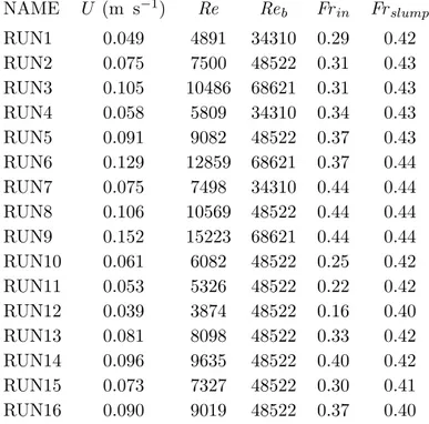
NAME ρ0 ρ1 g0′ h0 x0 R θ (kg m−3) (kg m−3) (m s−2) (m) (m) ( ) (◦) RUN1 1000 1015 0.15 0.200 0.100 2 0.0 RUN2 1000 1030 0.29 0.200 0.100 2 0.0 RUN3 1000 1060 0.59 0.200 0.100 2 0.0 RUN4 1000 1015 0.15 0.200 0.200 1 0.0 RUN5 1000 1030 0.29 0.200 0.200 1 0.0 RUN6 1000 1060 0.59 0.200 0.200 1 0.0 RUN7 1000 1015 0.15 0.200 0.400 0.5 0.0 RUN8 1000 1030 0.29 0.200 0.400 0.5 0.0 RUN9 1000 1060 0.59 0.200 0.400 0.5 0.0 RUN10 1000 1030 0.29 0.200 0.100 2 1.4 RUN11 1000 1030 0.29 0.200 0.100 2 2.5 RUN12 1000 1030 0.29 0.200 0.100 2 5.0 RUN13 1000 1030 0.29 0.200 0.200 1 1.4 RUN14 1000 1030 0.29 0.200 0.300 0.67 1.4 RUN15 1000 1030 0.29 0.200 0.200 1 2.5 RUN16 1000 1030 0.29 0.200 0.300 0.67 2.5

(34)

NAME U (m s−1) Re Reb Frin Frslump RUN1 0.049 4891 34310 0.29 0.42 RUN2 0.075 7500 48522 0.31 0.43 RUN3 0.105 10486 68621 0.31 0.43 RUN4 0.058 5809 34310 0.34 0.43 RUN5 0.091 9082 48522 0.37 0.43 RUN6 0.129 12859 68621 0.37 0.44 RUN7 0.075 7498 34310 0.44 0.44 RUN8 0.106 10569 48522 0.44 0.44 RUN9 0.152 15223 68621 0.44 0.44 RUN10 0.061 6082 48522 0.25 0.42 RUN11 0.053 5326 48522 0.22 0.42 RUN12 0.039 3874 48522 0.16 0.40 RUN13 0.081 8098 48522 0.33 0.42 RUN14 0.096 9635 48522 0.40 0.42 RUN15 0.073 7327 48522 0.30 0.41 RUN16 0.090 9019 48522 0.37 0.40

(35)

2.2.1 Analysis of the LES resolution

A preliminary analysis of the numerical results is performed in order to test the effectiveness of the model implementation as wall-resolving LES. A wall-resolving LES is defined as a simulation where the near wall streaks are directly resolved during the simulation. At the wall, the contribution of the Reynolds stresses is null, and the wall shear stress is totally related to the viscous part. Thus, following the considerations in Pope [2000] for a fully developed turbulent channel flow with a velocity Uc and a vertical dimension Hc, the wall shear stress τw can be defined as

τw = ρν ( d⟨Uc⟩ dy ) y=0 (2.16) The velocity scale and the length scale in the wall region, accounting for the viscosity and the wall shear stress, are the friction velocity uτ and viscous length scale δν, deﬁned as

uτ = √ τw ρ (2.17) and δν = ν uτ (2.18) The quantity y+_{is the distance from the wall measured in wall units: y}+₌

y/δν.

In a channel flow, it is possible to identify different regions basing on the y+ values. Namely, for y+ _{less than 50 the viscosity affects the flow dynamics,}

and the viscous wall region is defined. For higher values of y+ viscosity can be neglected and the region is called outer layer. When y+ < 5 the Reynolds shear stress is totally negligible if compared to the viscous one, and the viscous sublayer is identified. The log-law region is found from values of y+ > 30 up to part of the outer layer, where the mean velocity profile follows the von Kármán logarithmic power law. Finally, the region between the viscous sublayer and the log-low region (5 < y+ < 30) is commonly referred to as buffer layer. Figure 2.2 reports the division between layers varying y+, as shown in Pope [2000].

In order to correctly simulate the wall region, the use of about 8 grid points within the first 10 wall units in the wall-normal direction is commonly required and the first grid point would be located at about the first wall unit. Moreover, streaky structures generally have a characteristic spacing between 80 and 120 δnu, and a length of the order of 1000 δnu [Pope, 2000]. For the

(36)

Figure 2.2: Schematization of the wall regions deﬁned in terms of y+[Pope, 2000].

correct visualization of a streak, about 4 grid points and 20 grid points are required in the spanwise and in the streamwise directions. In this view, it is possible to deﬁne the dimensionless grid spacings

∆x+= ∆x uτ ν = ∆x δnu (2.19) ∆y+= ∆y/2 uτ ν = ∆y δnu (2.20) ∆z+= ∆z uτ ν = ∆z δnu (2.21) ∆x+, ∆y+ and ∆z+, in a wall resolving LES, should be respectively of the order of 50 (1000 δnudivided by 20 grid points) , 1 and 20 (80 δnudivided by 4 grid points), in order to exhaustively solves the viscous sublayer and to visualize the streaky structures.

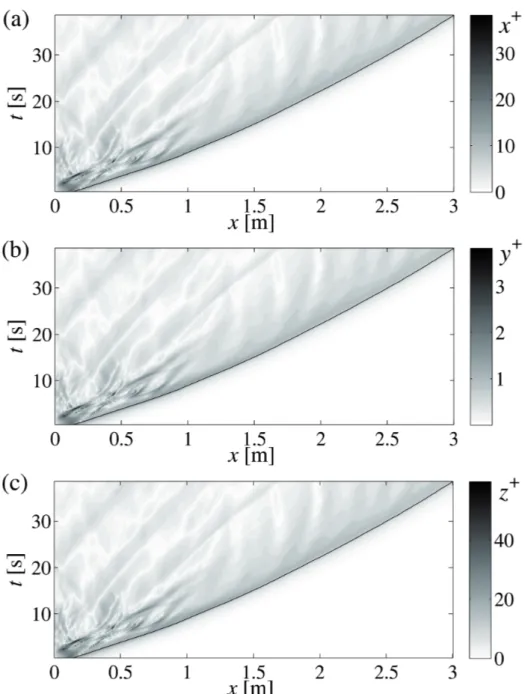
The maximum values of ∆x+, ∆y+ and ∆z+ are reported in Table 2.5 for each simulation. It is worth to mention that these values are obtained at an x-location close to the left wall of the tank, at the beginning of the simulations. These high values, indicating a non-optimal resolution for a canonical wall-resolving LES, occur when the lock ﬂuid collapses on the bottom surface and generates high values of the wall shear stress, especially close to the nose region. In Figures 2.3(a), (b) and (c) the contour plots of the values of ∆x+_{, ∆y}+_{and ∆z}+_{for RUN2, in dependence of x and t, are shown}

as representative of the overall trend observed in all the simulations. The black lines drawn in the ﬁgures are the position of the front of the current, xf. It is clear from the ﬁgure that high values of uτ, and consequently

(37)

the relevant values of the grid spacings, are found only at particular x-location and at particular times, i.e. at the beginning of the simulation. High values of uτ are also visible in correspondence of the nose of the gravity current during all the simulation, while in the rest of the body of the current negligible values of uτ are found. For this reason, the maximum values of ∆y+in correspondence of the times at which the gravity current has reached diﬀerent x-axis locations (x = 0.75 m, x = 1 m, x = 1.5 m and x = 1.75 m) are reported in Table 2.5. For example in RUN2, ∆x+ = 39.6, ∆y+ = 4.0 and ∆z+_{= 61.8 at the beginning of the simulation; then, when the current}

front reaches a distance on the x-axis of 1 m from the left wall of the tank, the resolution increases to ∆x+= 23.7, ∆y+= 2.4 and ∆z+= 37.0; ﬁnally, as soon as the front of the gravity current reaches half the length of the tank the resolution becomes 17.2, 1.7 and 26.9, in the three directions respectively, until the end of the simulation.

The goodness of the grid resolution is inversely proportional to Reb. Thus, cases characterized by g′₀=0.15 work better than RUN2, while the cases with g′₀=0.59 are worse. In the cases with smaller R the higher values of uτ last longer in space. Finally, in the up-sloping cases, as higher is θ, as smaller are the dimensionless grid spacings and, thus, the resolution is better. Note that the requirements of wall-resolving LES are based on the analysis of an equilibrium boundary layer, where fully developed streaks are present. It must be considered that the higher values of the dimensionless grid spacings are only occasional and local values, i.e. they are veriﬁed only at particular times and x-locations, and thus the areas over which the under-resolution occurs are small and rare (Figure 2.3). Moreover, the present ﬂow exhibits transitional and non-equilibrium conditions. Consequently, looking at the Figure 2.3, the resolution employed in the present study can be considered enough, because, although the maximum values reported in Table 2.5, during most of the duration of all the simulations a ∆y+ of the order of 1 is found.

(38)

Figure 2.3: Analysis of the grid resolution for RUN2: (a) ∆x+_{; (b) ∆y}+_{; (c) ∆z}+_. Values are plotted versus time and versus x-axis location.

(39)

NAME ∆x+ ∆y+ ∆z+ ∆y+ ∆y+ ∆y+ ∆y+ xf= xf= xf= xf= 0.75 m 1 m 1.5 m 1.75 m RUN1 27.0 2.7 42.2 2.2 1.8 1.2 1.2 RUN2 39.6 4.0 61.8 3.5 2.4 1.7 1.6 RUN3 51.9 5.2 81.1 4.6 2.7 2.2 2.0 RUN4 27.1 2.7 42.4 2.7 2.6 1.6 1.5 RUN5 33.9 3.4 53.0 3.4 2.9 2.0 1.9 RUN6 45.0 4.5 70.3 4.3 4.2 2.8 2.5 RUN7 25.7 2.6 40.1 2.6 2.6 2.5 1.9 RUN8 37.1 3.7 57.9 3.7 3.7 2.7 2.3 RUN9 47.2 4.7 73.8 4.7 4.7 4.3 2.8 RUN10 34.6 3.4 54.1 3.0 2.1 1.5 1.4 RUN11 32.1 3.2 50.2 2.9 2.2 1.5 1.3 RUN12 35.4 3.5 55.4 2.2 1.8 1.5 1.4 RUN13 33.7 3.4 52.6 3.4 2.8 2.1 1.9 RUN14 34.5 3.5 53.9 3.5 3.5 2.4 2.2 RUN15 33.5 3.4 52.3 3.4 2.8 2.1 1.9 RUN16 34.6 3.5 54.0 3.5 3.5 2.4 2.2

(40)

2.3 Numerical results and comparison with the

experiments

In order to assess the reliability of the numerical model, the comparison be-tween the laboratory experiments and the corresponding numerical simula-tions is presented in this section. The development of a lock-released gravity current can be considered essentially a two-dimensional phenomenon, with three dimensional effects developing in the cross-sectional plane being negli-gible compared to the main two-dimensional features. In the laboratory, to detect the main features of front position, a side-view of the advancement in time of the current is recorded during each laboratory experiment. On the other hand, three-dimensional LES are realized. Thus, in order to make comparisons between LES and experiments and in order to perform part of the post-processing of LES data, statistics are accumulated averaging along the spanwise direction of homogeneity. This operation is denoted with the symbol⟨ ⟩. The numerical dimensionless density field, ρ∗, is defined as

ρ∗(x, y, z, t) = ρ(x, y, z, t)− ρ0 ρ1− ρ0

(2.22) An example of the spanwise averaged dimensionless density field ⟨ρ∗⟩ is shown in Figure 2.4. Different profiles can be chosen to define the interface between the gravity current and the ambient fluid: six levels are adopted (as in Hacker et al. [1996]) in the color-map of Figure 2.4 (0.02≤ ⟨ρ∗⟩ < 0.05, 0.05 ≤ ⟨ρ∗⟩ < 0.20, 0.20 ≤ ⟨ρ∗⟩ < 0.40, 0.40 ≤ ⟨ρ∗⟩ < 0.60, 0.60 ≤ ⟨ρ∗⟩ < 0.80 and 0.80 ≤ ⟨ρ∗⟩ ≤ 1). In this work the interface is defined by the iso-density level corresponding to⟨ρ∗⟩ = 0.02. The influence of the iso-density threshold chosen to define the interface between the gravity current and the ambient fluid will be further discussed in the following of this thesis. The comparison between the numerical and the experimental front position is made, together with an analysis of the main features of the current in-ferred from the observation of its shape. The front position of the current xf is defined as the streamwise coordinate of the nose of the dense current (black dot in Figure 2.4), at a distance of 4 mm from the bed. This vertical distance was chosen in order to make the numerical results comparable with the space dimensions detectable by the resolution of the camera recording the laboratory experiments. The experimental front position is obtained by applying the threshold analysis of the grey levels of the images and following the time-advancement of the first point close to the bottom, detected as a pixel belonging to the nose of the current. The different phases of devel-opment of the gravity currents [Simpson, 1997] are also studied, and the

(41)

Figure 2.4: Spanwise averaged dimensionless density ﬁeld: interface taken at

⟨ρ∗_{⟩ = 0.02; iso-density levels deﬁned with ⟨ρ}∗_{⟩ = 0.05, ⟨ρ}∗_{⟩ = 0.2,}

⟨ρ∗_{⟩ = 0.4, ⟨ρ}∗_{⟩ = 0.6 and ⟨ρ}∗_{⟩ = 0.80. The front position of the}

gravity current is shown by the black dot.

dimensionless front position x∗_f and the dimensionless time T∗ are deﬁned as: x∗_f = xf(t)− x0 x0 (2.23) T∗ = t ub x0 (2.24) The comparison between laboratory measurements and numerical simula-tions in terms of the front velocity is presented in the following paragraphs, emphasizing the inﬂuence of the parameters varied herein.

A qualitative comparison between the gravity currents obtained by labo-ratory experiments and the corresponding numerical simulations was also performed, when available. For instance, Figure 2.5 shows the experimental frames captured during EXP2 (left part of the panel) and the contour maps of⟨ρ∗⟩ for RUN2 (right part of the panel) at the same times. The main fea-tures of the numerical gravity current are similar to the experimental ones. The position of the dense current along the x-axis is well reproduced by the numerical model, as well as the shape of the interface between the two fluids. Advancing in time, the dense current mixes with the ambient fluid, decreas-ing in density. The thickness of the head of the current decreases with time, while the tail region increases in length and becomes thinner. Both in the experimental and in the numerical images Kelvin-Helmholtz billows are vis-ible. These instabilities form at the interface between the two fluids due to the velocity shear and characterize the slumping phase [Figures 2.5(a), (b)]. In the self-similar phase, they lose their coherence and a smoother interface between the dense and the light fluid is observed [Figures 2.5(c), (d), (e), (f)]. Similarly, a good agreement between the numerical density fields and

(42)

Figure 2.5: Experimental frames of EXP2 (left hand side of the panel) and⟨ρ∗⟩

of RUN2 (right hand side of the panel) at diﬀerent times: (a) and (b)

T∗ ∼= 17.1; (c) and (d) T∗ ∼= 38.6; (e) and (f) T∗∼= 65.9; (g) and (h)

T∗∼= 90.0.

the experimental images was found in the other cases here analysed (not shown).

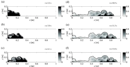
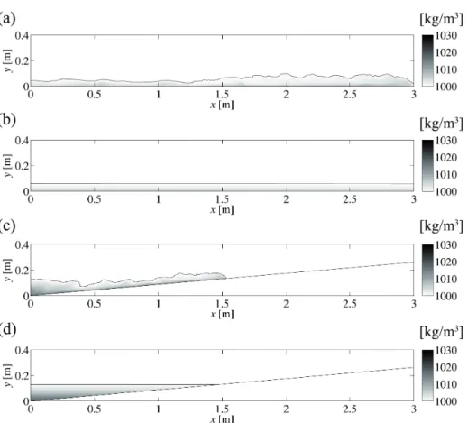
Experimental density fields were also evaluated following the procedure de-scribed in section 2.1.1. Figures 2.6 and 2.7 show the experimental and the numerical density fields evaluated for EXP3 and RUN3, respectively. The iso-density lines plotted in both the figures refers to levels of ⟨ρ∗⟩= 0.02, ⟨ρ∗_{⟩= 0.05, ⟨ρ}∗_{⟩= 0.08, ⟨ρ}∗_{⟩= 0.1, ⟨ρ}∗_{⟩= 0.2 and ⟨ρ}∗_{⟩= 0.5. Some} differ-ences can be observed in the area between the body and the tail regions of the gravity current, which in the numerical simulation appears to be more abrupt than in the experiments. Nevertheless, a very good agreement can be observed between the Figures 2.6 and 2.7. In the first time shown it is possible to observe the presence of a KH billow at the x-axis location corre-sponding to x = 0.5 m, that occurs both in the experiment [Figure 2.6(a)] and in the numerical simulation [Figure 2.7(a)]. The densest part of the gravity current, bounded by the iso-density level ⟨ρ∗⟩= 0.5 and visible as dark-black coloured area [Figures 2.6(a) and 2.7(a)], starts to dilute in the following times [Figures 2.6(b) and 2.7(b)]. Advancing in time, the dense

(43)

Figure 2.6: Dimensionless density ﬁeld⟨ρ∗⟩ for EXP3 (g0′ = 0.59 and R = 2) at diﬀerent times: (a) T∗ = 20.4, t = 6 s; (b) T∗ = 44.1, t = 13 s; (c)

T∗ = 72.2, t = 21 s; (d) T∗ = 92.1, t = 27 s. The iso-density levels drawn correspond to ⟨ρ∗⟩= 0.02, ⟨ρ∗⟩= 0.05, ⟨ρ∗⟩= 0.08, ⟨ρ∗⟩= 0.1,

⟨ρ∗_{⟩= 0.2 and ⟨ρ}∗_{⟩= 0.5.}

current mixes with the ambient ﬂuid, and the magnitude of the areas cor-responding to density values of ⟨ρ∗⟩= 0.2, clearly visible in Figures 2.6(b) and 2.7(b), gradually decreases in Figures 2.6(c) and 2.7(c). At the end of the experiment, lower and more homogeneously distributed values of the dimensionless density ﬁeld are visible in the body of the gravity current, for both EXP3 and RUN3 [Figures 2.6(d) and 2.7(d)].

Diﬀerences between the numerical results and the observed experiments are inevitably associated to the eﬀects of the gate removal, which is far from the numerical ideal operation, as well as to the boundary conditions imposed in the model, which are similar but not equal to the experimental condi-tions. Nevertheless, it is possible to assert that a good agreement between simulations and experiments is found.

(44)

Figure 2.7: Dimensionless density ﬁeld⟨ρ∗⟩ for RUN3 (g′₀= 0.59 and R = 2) at diﬀerent times: (a) T∗ = 20.4, t = 6 s; (b) T∗ = 44.1, t = 13 s; (c)

T∗ = 72.2, t = 21 s; (d) T∗ = 92.1, t = 27 s. The iso-density levels drawn correspond to ⟨ρ∗⟩= 0.02, ⟨ρ∗⟩= 0.05, ⟨ρ∗⟩= 0.08, ⟨ρ∗⟩= 0.1,

(45)

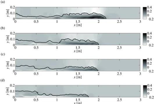
2.3.1 Inﬂuence of R and g′₀ on the front position

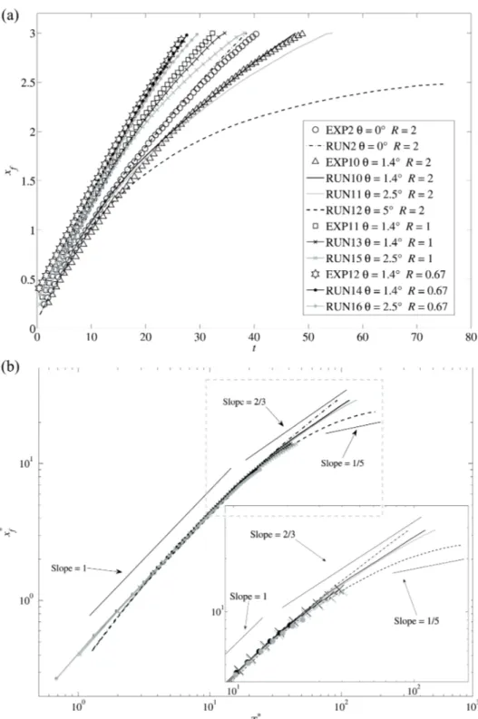
The numerical and the experimental xf versus time are shown in Figure 2.8 for the experiments EXP1 ÷ EXP9 and the corresponding numerical simu-lations RUN1 ÷ RUN9. Namely, in Figure 2.8(a) the front positions of the gravity currents for the cases in which the configuration of the fluid in the lock at t = 0 is vertically-oriented (R = 2) are displayed. Figure 2.8(b) re-ports the comparison of xf(t) for the cases characterized by a square-shaped initial lock fluid volume (R = 1). Finally, in Figure 2.8(c), the advancement of the fronts for the gravity currents with the horizontally-oriented initial lock fluid volume are presented (R = 0.5). In the figure, initial density differences of 15 kg/m3 are represented by square markers and solid lines. g′₀ = 0.29 cases are shown with circles and dash-dot lines. Triangle mark-ers and dashed lines are for the g′₀ = 0.59 cases. As expected, for fixed R, gravity currents with high g₀′ are faster than the currents with low g₀′. Furthermore, focusing on cases with the same initial density difference, the velocity of gravity currents is higher as R decreases. This is also visible looking at the values of Frslump in Tables 2.2 and 2.4, which represent the dimensionless slumping velocity of the different cases. For EXP1÷EXP9 Frslump is about 0.41 for R = 2, Frslump ∼ 0.46 R = 1 and Frslump ∼ 0.47 for R = 0.5 (Table 2.2). A similar trend occurs also in the numerical sim-ulations (Table 2.4). Moreover, in Figure 2.8, the curves of xf(t) are more bent in the vertically-oriented cases than in the horizontally-oriented ones. In fact, the front positions in Figure 2.8(c) are represented by straight lines, indicating a constant front velocity and the development of the slumping phase only. A good agreement between the numerical and the experimental front positions of the gravity currents is evident from the Figure 2.8. The different flow regimes of the gravity currents are discernible analysing the dimensionless front position x∗_f (defined in equation 2.23) versus the di-mensionless time T∗(equation 2.24) in a log-log plot [Rottman and Simpson, 1983]. Since the agreement between the laboratory experiments and the nu-merical simulations is good, and since all the nine x∗_f(T∗) collapse in one curve independent of g₀′, only the numerical results with g₀′ = 0.29 (RUN2, RUN5 and RUN8) are plotted in Figure 2.9 as examples. As discussed above, the propagation of a gravity current over a horizontal bed, accord-ing to the shallow-water theory, is commonly divided in different phases of spreading [Rottman and Simpson, 1983], namely a slumping phase, a self-similar phase and a final viscous phase. When the gate dividing the dense and the light fluids is removed, the a gravity current forms and starts mov-ing downstream.

(46)

Figure 2.8: Numerical and experimental front position versus time: (a) R = 2;

(b) R = 1; (c) R = 0.5. Square markers and solid lines correspond to the g₀′ = 0.15 cases, circles and dash-dot lines label the g₀′ = 0.29 cases, triangle markers and dashed lines are for the g₀′ = 0.59 cases

(47)

During the first phase of spreading, the front of the current moves at a con-stant velocity value and the slumping phase occurs. During this phase the bore and the current travel together downstream, and x∗_f increases linearly in time. The slumping phase is clearly visible in all the simulated cases, and it is well approximated by the linear function with angular coefficient equal to 1 (dashed line in Figure 2.9). Subsequently, when the bore reaches the nose of the current and overtakes it, a change in the dynamics of the flow occurs, and the transition to the self-similar phase takes place. During this second phase the current slows down and x∗_f follows the theoretical power law of t2/3. As expected, all the gravity currents slow down during the self-similar phase both in the simulations and in the experiments. The thin solid line with a slope = 2/3 in Figure 2.9 indicates the theoretical trend. The agreement with the theory is not complete, but a fair approximation of the theoretical 2/3 power law is visible both for the R = 2 and for the R = 1 cases. It must be underlined that the 2/3 power law was deducted from the analysis of horizontally-oriented cases, thus it does not work perfectly when R = 2. The limited length of the tank does not allow a complete develop-ment of the self-similar phase, neither for the gravity currents characterized by R = 1 nor for the ones with R = 0.5. Due to the same geometrical constrains, the viscous phase does not occur in these experiments and the front of the gravity current reaches the downstream wall of the tank before the viscous forces influence the flow dynamics. Thus, varying R, different flow regimes are reached at the end of each experiment. This implies that the cases with different R only show different durations of the same phe-nomenon and, for what concerns x∗_f(T∗), it is apparent that the influence of R is negligible for all the slumping and for the early beginning of the self-similar phases. In addition, since not even the effect of the variations of g₀′ is visible in the dimensionless plot of x∗_f, all the functions x∗_f(T∗) of the experiments from EXP1 to EXP9 collapse on the same curve.

(48)