The Italian regional dualism: A MARS and panel data analysis

(1)

© Southern Regional Science Association 2018. ISSN 1553-0892, 0048-749X (online)

www.srsa.org/rrs

The Review of Regional Studies

The Official Journal of the Southern Regional Science Association

The Italian Regional Dualism: A MARS and Panel Data Analysis

*

Iacopo Odoardia_{and Fabrizio Muratore}b

a_{Department of Philosophical, Pedagogical, and Economic-Quantitative Sciences, University of Chieti-Pescara, Italy} b_{National Foundation of Accountants, Economics, and Statistical Office, Italy}

Abstract: The income gap between the richest and the poorest areas in Italy has increased in the last decades. We study the sources of regional wealth that can explain the differences in income and compare rich and poor areas to provide suggestions on how to bridge the gap. A multivariate adaptive regression splines (MARS) analysis is used to detect the relevant GDP determinants, and a fixed effects model is used to investigate the regional characteristics. The effects of the 2007 crisis are evident in all regions, and some structural weaknesses in the less wealthy areas limit the opportunities to exit the recession and close many socioeconomic gaps with the wealthiest regions.

Keywords: North-South problem, regional inequality, MARS, panel data, regional policy JEL Codes: O15, R11, O18

1. INTRODUCTION

Many countries are characterized by strong regional disparities due to unequal development opportunities in different local socioeconomic contexts. Economic studies refer to these inequalities as North-South problems (Williamson, 1965). An evident dualism between areas of a country is present in many advanced economies, and despite signs of convergence at least until the 1980s (Barro and Sala-I-Martin, 1991), it seems that the risk of an increasing divergence is still a problem. Among the most studied cases, many refer to the coastal/inland dualism in China (Lin, Lin, and Ho, 2013; Li and Fang, 2014), the North/South differences in the U.S. (Tsionans, 2000; Caselli and Coleman, 2001), and the differences between the rich South and the relatively poor North of England (Martin, 1988; Dunford, 1995). Among the best-known cases, Italy is characterized by a strong regional dualism (Etzo, 2011) that is observable in the divergence between two economically opposite areas, in which some of the richest northern regions have an average income equal to almost twice that of the southern area.

The aim of this work is to investigate the causes of different income levels among the Italian regions by highlighting the local sources of wealth. In this paper, the reasons for the progressive distancing of the average incomes are sought through the study of 19 regressors that influence the GDP per capita. We compare the divergent macro areas using data on the 20 Italian regions for the period 2004–2013, thus including the crisis period and the subsequent recession.

Therefore, we do not test the dynamics of the well-known β and σ convergences (as in Azzoni (2001) for Brazil) as is often done in studies on regional gaps. In Italy, the North-South

*_{Acknowledgements. The authors want to thank the editor, Amanda Ross, and two anonymous referees for their valuable} comments.

Odoardi is Research Fellow in Economics at the University of Chieti-Pescara, Pescara, Italy. Muratore is a statistician at the National Foundation of Accountants, Rome, Italy. Corresponding Author: I. Odoardi E-mail: iacopo.odoardi@unich.it.

(2)

differences have grown in the last decades, and only club convergence within macro areas is recognized (Brida, Garrido, and Mureddu, 2014), while the strongest convergence process is present only among the wealthiest regions (Arbia and Basile, 2005). Even in the estimation of transnational clubs, the distance between areas is high: northern Italy joins the Central Europe group, and the southern area is in the group with the less wealthy regions of Greece, Spain, and Portugal (Von Lyncker and Thoennessen, 2017). Furthermore, the North-South income gap in Italy has worsened after the crisis of 2007 (Lagravinese, 2015).

Our approach to regional analysis consists of different related steps. Considering the North-South divergence as widely tested in the economic literature, our analysis starts with a selection of 19 variables covering various mutually related aspects of the local development processes. We divide the regions into homogeneous clusters according to the characteristics of the period under study for the models’ application because a proper grouping is essential for the regional analysis of the Italian context (as suggested by Terrasi, 1999). The grouping allows us to determine which regions form what the literature defines the “rich North” and the relatively “poor South.” In the first step, we exploit the knowledge present in a vast dataset using a MARS (multivariate adaptive regression splines) model that has the capability to determine relevant variables (Friedman, 1991). We apply MARS to these proper groups of regions to select the significant variables in each area with respect to the target variable, i.e., the GDP per capita. Subsequently, we control for the effect of unobserved heterogeneity using a panel data model, considering the relevance of the latter model as suggested by Arbia and Basile (2005) in a study on the convergence of the Italian provinces.

Although the MARS model is widely used in several scientific areas and one of its main purposes is to select important variables in large datasets, based on our knowledge, it has not been used in regional studies in combination with panel data techniques. The use of MARS in economics is not yet widespread, though this technique has been demonstrated to be more efficient than several econometric techniques, and it can find deeper relationships between variables. The efficiency of the MARS model was examined by Abraham, Steinberg, and Philip (2001), who compared MARS with recent models of soft computing (see also the model comparison in Fattahi, 2011).

Our contribution is twofold. First, we seek local sources of wealth to contribute to the understanding of the reasons of regional divergence. Second, our methods use the capabilities of different models with useful features to obtain more information from the data and their relationships with a complex variable such as GDP.

The contribution of MARS is important both to reduce econometric problems in the dataset (e.g., multicollinearity) and to find unobserved relationships among the variables. MARS is used when, for example, nonlinear relationships exist in the data or many explanatory variables related to the studied phenomenon are used. Thus, one of the innovative aspects of this work is the opportunity to consider a broad set of variables suggested by regional studies for the Italian context and take advantage of this non-parametric technique that can analyze them jointly to efficiently detect the most important ones.

From the results and comparing the findings of the economic literature on the Italian dualism, we draw policy suggestions with the aim of encouraging convergence. In fact, the comparison between areas can suggest the points for intervention to correct the negative performances of the relatively poorest area and try to bridge the socioeconomic gaps. In our

(3)

findings, structural weaknesses in the southern area are highlighted, while only some aspects of the North’s development deserve to be imitated during the knowledge economy era, thus favoring a common growth path for the regional convergence. The need to exploit local features is evident, but long-term growth must take into account both the knowledge economy characteristics and Italy’s role in the globalized economy. For both of these aspects of development, South Italy is still struggling.

The next section provides an overview of the Italian context; Section 3 outlines the methods used, and the variables are presented in Section 4. Section 5 shows the division of the regions into macro areas, and in Section 6, we propose the MARS and the fixed effects model results. In the last section, we discuss our results with the aim of proposing policies to encourage growth in the less wealthy area, drawing on what works well in the most developed regions.

2. SOME ASPECTS OF THE ITALIAN NORTH-SOUTH DIVIDE

The presence of large disparities in GDP among areas of the same country is a well-known problem in economics. The economic and social gaps between North and South, which are classified as “rich” and “poor” areas, characterize many contexts. In 1965, Williamson described the North-South problem as a widespread question in almost all developed countries and without a common explanation because of the lack of studied relationships between regional inequalities and the national development process. The strong differences suggest investigating two distinct geographical contexts (the above described North-South, coastline-hinterland, etc.).

Evident differences in the local economic development processes have been present in Italy since the unification of the country in 1861 (Daniele and Malanima, 2007), while some traces of income convergence were observed until the 1980s (Barro and Sala-I-Martin, 1991). Development paths have always been different between the North, which was industrialized and close to the European markets, and the South, which was initially agricultural, plagued by inefficiencies and clientelism, and characterized by poor economic performance despite decades of extraordinary public interventions (Felice, 2007). Growth opportunities were therefore influenced both by the endowment of natural resources and by the different social and cultural capital at the local level.

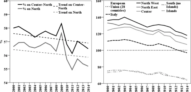
Even the different rates of economic growth affect the divergence (see Islam, 2003). For the Italian case, the average variation in the GDP per capita (constant 2010 values) in the period 1996–2014 was 0.08 percent for the North, 0.1 percent for the Center, and 0 percent for the South (our elaborations on Istat data). Gaps are then more difficult to fill; the South grows less than the North, and the differences are evident in Figure 1 showing the GDP per capita of the South as a percentage of those of the Center-North and of the North. In Figure 1, the decreasing trends show that the income of the “poor” is ever more distant from that of the “rich.” This difference is also observed from the comparison of the GDP of the Italian macro-areas with the European average GDP in the right graph.

It is evident that the first negative effects of the import crisis (peak in 2009, left graph) hit the northern area that is more exposed to exogenous influences, but the foreign markets have permitted the faster recovery compared with the South (see the minimum values of the ratios in 2011––2014). The North-South differences are even more evident in the right graph, observing the positioning of the macro areas above and below the European average GDP per inhabitant (horizontal dotted line). The differences are due to the opening to international markets, the

(4)

Figure 1: GDP Per Capita (at Market Prices, Constant 2010 Values) of the South of Italy as a Percentage of the Other Macro Areas (Left Graph) and GDP Per Inhabitant (at Current

Prices) of the Italian Macro Areas on the Basis of the EU Average (=100, Right Graph)

Source: Authors’ elaboration based on Istat and Eurostat data.

disposable physical and human capital, and the entrepreneurial vitality. However, the endowment of social capital and the societal structure are also different and help to explain the persistent gaps in income and productivity (Helliwell and Putnam, 1995). Other effects exist: for Alesina, Danninger, and Rostagno (1999), the large presence of public employment (considered as a redistributive device) and other types of subsidies discourage market linked activities in the South, and the organization of the local welfare state is inefficient in the southern area because of historical weaknesses and recent political errors (Fargion, 1996).

In contrast, positive effects could arise from the existing relationships between regions or from the possible mobility of productive factors. For example, according to Pedroni and Yao (2006), the income differences in China are due to interprovincial labor (and factor) mobility, in addition to geographic factors and market openness. In Italy, the mobility (or the propensity to migrate) represents a problem particularly in southern area because of its related costs, demographic factors (e.g., the aging of the population), and the scarce efficiency in the matching of demand/supply of labor among these regions (Faini et. al., 1997).

3. METHODS

Our analysis concerns different steps. After a proper division of the Italian regions based on the current socioeconomic characteristics to represent the North-South dualism, we apply a MARS model to select the relevant variables for each group. Then, we apply a fixed effects model to examine dependency relationships with local GDP.

3.1 MARS Model

Multivariate adaptive regression splines analysis is a technique widely used in many areas of study and increasingly exploited in the economics field for its ability to manage data complexities efficiently, particularly when there are complex relationships between data and

(5)

non-© Southern Regional Science Association 2018.

linearity in interactions. Such complexity is present between a multifaceted variable representing economic growth and the many factors influencing it, as tested by Annoni and Rubianes (2016) for 268 European regions. The authors also suggest the application of MARS method as an efficient opportunity to model complex relationships (as expressed by Varian, 2014). Deichman et. al. (2002) demonstrate the greater efficiency of MARS compared to logistic models on marketing strategies. Zareipour, Bhattacharya, and Canizares, (2006) use MARS to forecast the hourly energy price because this technique is considered adequate when a large number of explanatory variable candidates need to be included in the analysis. Lee and Choi (2011) use MARS to observe the nonlinear relationship between the effects of speculative house flippers on housing prices.

Some tests have been made in applying this method to regional gaps (Chen et. al., 2018; Odoardi et. al., 2018), while our analysis is composed of more steps. We use MARS to detect important variables in a large dataset (see Hastie, Tibshirani, and Friedman, 2001) that allows us to simultaneously test the role of many variables (see the model comparison for the important variables in Mina and Barrios, 2010). A panel data analysis is used for further investigations, considering the strong regional complexity in Italy.

In synthesis, MARS model is an application of techniques for solving regression-type problems, and its objective is to estimate the values of a dependent variable from a set of predictors considering a non-parametric regression technique. A positive aspect in our study on the GDP is that a non-parametric modeling approach does not need to identify the functional relationship between the target and the independent variables.

MARS was proposed by Jerome H. Friedman (1991) to organize the relationships between several input variables and a target variable. The training datasets are partitioned into separate piecewise linear segments (splines) of differing gradients (slope). The splines are connected efficiently, and the piecewise curves (polynomials, that are the so-called basis functions) result in a flexible model.

It is possible to have collinearity between some variables and MARS can help solve the problem thanks to the two phases that constitute the model: the forward pass and the backward pass. The forward pass phase builds an overfit model that has a good fit to the data. The backward pass prunes the model to achieve a better generalization ability. It considers the terms individually, removing the least effective term until it finds the best submodel. The backward pass can choose any term to delete, whereas the forward pass can only see the next pair of terms at each step. Therefore, the MARS technique does automatic variable selection (it includes important variables in the model and excludes unimportant ones) that avoids arbitrariness in the selection, particularly in the presence of collinearity and concurvity (see also Friedman, 1993).

MARS constructs the functional relation from a set of coefficients and basis functions that depend on the dataset used in each case (see Felicisimo et. al., 2013). Therefore, the relationship is additive and interactive, involving fewer variable interactions (Lee et. al., 2006). This model uses two-sided truncated functions of the form ±(𝑥𝑥 − 𝑡𝑡)₊ as basis functions for linear or nonlinear expansion, which approximates the relationships between the response and predictor variables.

If we consider the GDP per capita as 𝑦𝑦 and a matrix of 𝑝𝑝 input variables as 𝑋𝑋 = �𝑋𝑋1, … , 𝑋𝑋𝑝𝑝�, the model is:

(6)

in which 𝑓𝑓 is the MARS model (containing basis functions that are spline piecewise polynomial functions), and 𝑒𝑒 is the fitting error. Piecewise linear functions must have the form 𝑚𝑚𝑚𝑚𝑥𝑥(0, 𝑥𝑥 − 𝑡𝑡), and the knot is defined at value 𝑡𝑡. The term max is used because the positive part is considered; otherwise, 0 is assigned. Then,

𝑚𝑚𝑚𝑚𝑥𝑥(0, 𝑥𝑥 − 𝑡𝑡) = �𝑥𝑥 − 𝑡𝑡, if 𝑥𝑥 ≥ 𝑡𝑡_{0, otherwise}

The basis functions have the form 𝐵𝐵_𝑚𝑚(𝑥𝑥) = 𝐼𝐼[𝑥𝑥 ∈ 𝑅𝑅_𝑚𝑚], in which 𝐼𝐼 is an indicator function with value 1 if its argument is true (otherwise it is 0), and they can obtain the multivariate equation in the form:

(2) 𝑓𝑓̂(𝑥𝑥) = ∑𝑚𝑚_𝑖𝑖=1𝑚𝑚_𝑚𝑚𝐵𝐵_𝑚𝑚(𝑥𝑥) .

The multivariate splines algorithm permits models from two-sided truncated functions of the predictors (𝑥𝑥) that are 𝑏𝑏_𝑞𝑞±(𝑥𝑥 − 𝑡𝑡) = [±(𝑥𝑥 − 𝑡𝑡)]₊𝑞𝑞. The basis functions generalize spline fitting to higher dimensions. The multivariate spline basis function has the form:

(3) 𝐵𝐵_𝑚𝑚(𝑞𝑞)(𝑥𝑥) = ∏ �𝑠𝑠_{𝑘𝑘𝑚𝑚}∙ �𝑥𝑥_{𝑣𝑣(𝑘𝑘,𝑚𝑚)}− 𝑡𝑡_{𝑘𝑘𝑚𝑚}��

+ 𝑞𝑞 𝐾𝐾𝑚𝑚

𝑘𝑘=1 .

The basis functions originate from recursive partitioning useful for selecting a small subset of regressor functions. Finally, a form of the MARS model (Friedman, 1991) is present in the Equation (4):

(4) 𝑓𝑓̂(𝑥𝑥) = 𝑚𝑚₀+ ∑𝑀𝑀_𝑚𝑚=1𝑚𝑚_𝑚𝑚∏ �𝑠𝑠_{𝑘𝑘𝑚𝑚}∙ �𝑥𝑥_{𝑣𝑣(𝑘𝑘,𝑚𝑚)}− 𝑡𝑡_{𝑘𝑘𝑚𝑚}��

+ 𝐾𝐾𝑚𝑚

𝑘𝑘=1 .

In Equation (4), 𝑚𝑚₀ is the coefficient of the constant basis function 𝐵𝐵₁, and the sum is over the basis functions 𝐵𝐵_𝑚𝑚 in Equation (3).

We calculate the generalized cross validation (GCV) error for each group of regions. This is a measure of the goodness of fit, considering the model complexity and the residual error:

(5) 𝐺𝐺𝐺𝐺𝐺𝐺 = ∑ �𝑦𝑦𝑖𝑖−𝑓𝑓(𝑥𝑥𝑖𝑖)�

2 𝑁𝑁

𝑖𝑖=1

�1−_𝑁𝑁𝐶𝐶�2

with 𝐺𝐺 = 1 + 𝑐𝑐𝑐𝑐, 𝑁𝑁 is the number of cases, and 𝑐𝑐 is the effective degrees of freedom, which is equal to the number of independent basis functions. The quantity 𝑐𝑐 is the penalty for adding a basis function (Hill and Lewicki, 2006).

3.2 Fixed Effects Model

We use a fixed effects model (FE) to find relationships between variables within groups (Elhorst, 2014) and control for unobservable heterogeneity. This model is used in regional studies, for example, on convergence influenced by migration (Ozgen, Nijkamp, and Poot, 2010) or by human capital, (Ramos, Suriñach, and Artís, 2010) and to study economic growth (Dall’Erba and Fang, 2015).

In the FE model, the individual effects are considered fixed and are included among the explanatory variables as individual constants. This technique imposes time-independent effects for each object that are possibly correlated with the regressors (Fitzmaurice, Laird, and Ware, 2004) if the fixed effects are assumed. FE can be considered an appropriate model because we consider all the Italian regions divided into groups, thus not a sample, and the number of regions is relatively small. For the panel data analysis, our equation can be written as:

(7)

(6) 𝐺𝐺𝐺𝐺𝐺𝐺_{𝑖𝑖𝑖𝑖} = 𝛽𝛽₀+ 𝛽𝛽₁𝑥𝑥_{𝑖𝑖𝑖𝑖}+ . . . +𝛽𝛽₁₉𝑥𝑥_{𝑖𝑖𝑖𝑖}+ 𝜀𝜀_{𝑖𝑖𝑖𝑖}

in which the regional GDP per capita is the dependent variable, and 𝑥𝑥_{𝑖𝑖𝑖𝑖} are the 19 independent variables (discussed in Section 4) for the 20 Italian regions (𝑖𝑖), considering the period 2004–2013 (𝑡𝑡). The stochastic error term is 𝜀𝜀_{𝑖𝑖𝑖𝑖}, while 𝛽𝛽₀, … , 𝛽𝛽₁₉ are the estimated parameters.

4. SELECTION OF THE VARIABLES AMONG THE CAUSES OF THE NORTH-SOUTH DUALISM

The variable that represents the level of economic development in studies on regional inequality and on the North-South problem is the GDP per capita. This variable is studied by Barro and Sala-I-Martin (1991) in a cross-country study on regional convergence considering the contribution of the various economic sectors (i.e. construction, manufacturing, service, etc.), and Jian, Sachs, and Warner (1996) consider the role played by the “coastal effect” to indicate how the opening to foreign markets is an important source of possible convergence of the GDP per capita in the Chinese provinces. We consider the regional GDP per capita (constant 2010 values, Istat data) as the target variable to have a direct comparison that is not affected by inflation.

In our analyses, a relevant group of independent variables refers to human capital. This important asset can explain part of the divergence in economic growth rates of different areas as observed by Démurger (2001). The economic role of human capital has been tested for decades (see Goldin, 2016) and represents one of the main competitive assets of advanced economies (Aghion and Howitt, 1998; Levine, 1998). The human capital endowment may be considered one of the most important economic assets in the regional income determination (Gennaioli et. al., 2013) together with other types of capital equipment and infrastructure (Fleisher, Li, and Zhao, 2010).

Human capital is significant in countries oriented to a high-quality production with high added value. This is possible thanks to the paths of education (Breton, 2013) and vocational training (Edwards et. al., 2002). Proxies of human capital linked to school and university education and lifelong learning must be considered. However, the positive effects of human capital are not immediately observable if other structural features do not co-exist to exploit the skills and capabilities of workers. The failure to fully exploit the investment in education may be caused, for example, by the scarcity of social and cultural capital (Throsby, 1999; De Graaf, De Graaf, and Kraaykamp, 2000).

These aspects could be relevant in the poorest areas of the country, showing that even the widespread presence of (public) higher education does not automatically influence the economic development through human capital enrichment. For example, a North-South gap in human capital exists in Italy for Abramo, D’Angelo, and Rosati (2016) because of the different quality and competitiveness of the universities.

Obviously, the level of human capital describes a qualitative aspect of the labor factor affecting its productivity level (Abel, Dey, and Gabe, 2012; Bowlus and Robinson, 2012) and therefore influencing the total factor productivity, as highlighted by Benhabib and Spiegel (1994). The productivity level is directly linked to the level of human capital (Fleisher, Li, and Zhao, 2010), and as studied by Gitto and Mancuso (2015), marked differences between the Center-North and the South are observed in the Italian case.

(8)

We also consider variables representing the characteristics of local businesses because these data are not often used in relation to GDP but are crucial in regional development (Van Stel, Carree, and Thurik, 2005). Furthermore, businesses’ characteristics are more important in the light of an effective North-South dualism in models of production because of the different level of industrialization (Imbriani et. al., 2014). North-South differences exist because of the natural characteristics and the proximity to foreign markets, which previously favored the location of businesses in the northern regions (A’Hearn and Venables, 2013).

Export values must also be included because export is one of the main components of aggregate demand, and according to Jian, Sachs, and Warner (1996), foreign trade is one of the most important opportunities for local development in China. Furthermore, export is linked to firms’ characteristics and can be a potential strength in southern Italy if encouraged through planning and exploiting local characteristics (Capello, 2016).

Finally, the last group of variables considers the role of the local financial systems. In fact, structural inefficiencies are present in regional financial markets, particularly in the South (Ferri and Messori, 2000), and the 2007 crisis has worsened the situation, causing a so-called credit crunch, in which it was more difficult to grant loans to consumer households and businesses.

4.1 List of Independent Variables

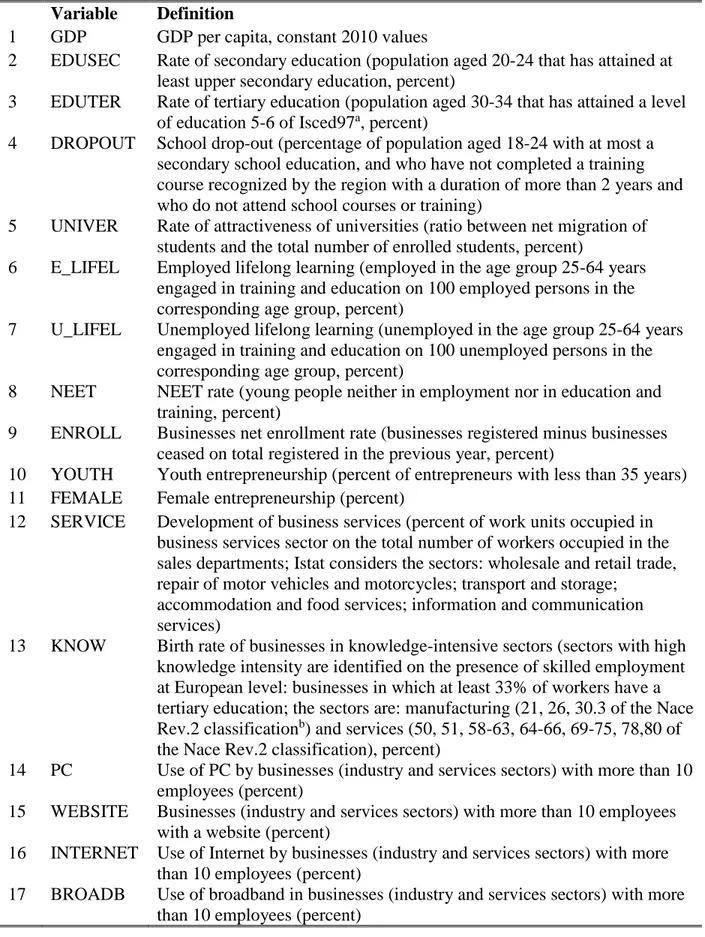
Variables that characterize the socioeconomic contexts of the regions and that are some of the causes of dualism are described in Table 1. The source of the data is Istat, the Italian National Institute of Statistics (Istituto Nazionale di Statistica), for the period 2004–2013. We consider the Istat data on “Territorial indicators for development policies.1” The first variable is the dependent variable; variables 2–8 concern human capital, and variables 9–20 concern businesses characteristics, export and the financial systems.

With regard to the chosen variables, an endogeneity problem can be present as discussed by Durlauf (2009) and others. This problem also occurs in models that are comparable with an augmented Solow model (Mankiw, Romer, and Weil, 1992). However, our aim is not to study economic growth but to seek the effective determinants of GDP. The presence of effects due to omitted variables (see Rose, 2001) is also possible.

In the selection of the variables, we do not consider similar or highly correlated independent variables that can cause redundancy. In addition, an excessive number of independent variables or long time series would lead to an overfitting problem (which could worsen the predictive capacity of the model).

5. CLUSTERING OF THE ITALIAN REGIONS

An official classification of the Italian regions in macro areas exists because of the historical, social, and economic evolution, and it is used by research and statistics institutions such as Istat and Eurostat. This traditional division compiles structural characteristics and common pathways of groups of regions that may no longer be valid, particularly in the period after the 2007 crisis. We apply two types of clustering analysis to have a correct grouping of the regions: factorial k-means and hierarchical. In the analysis, we consider all the independent variables and the GDP per capita with the aim of obtaining clusters that take into account many local aspects, in addition to regional wealth. We expect that the division between the geographical North and South will be

(9)

Table 1: Variable Descriptions Variable Definition

1 GDP GDP per capita, constant 2010 values

2 EDUSEC Rate of secondary education (population aged 20-24 that has attained at least upper secondary education, percent)

3 EDUTER Rate of tertiary education (population aged 30-34 that has attained a level of education 5-6 of Isced97a, percent)

4 DROPOUT School drop-out (percentage of population aged 18-24 with at most a secondary school education, and who have not completed a training course recognized by the region with a duration of more than 2 years and who do not attend school courses or training)

5 UNIVER Rate of attractiveness of universities (ratio between net migration of students and the total number of enrolled students, percent)

6 E_LIFEL Employed lifelong learning (employed in the age group 25-64 years engaged in training and education on 100 employed persons in the corresponding age group, percent)

7 U_LIFEL Unemployed lifelong learning (unemployed in the age group 25-64 years engaged in training and education on 100 unemployed persons in the corresponding age group, percent)

8 NEET NEET rate (young people neither in employment nor in education and training, percent)

9 ENROLL Businesses net enrollment rate (businesses registered minus businesses ceased on total registered in the previous year, percent)

10 YOUTH Youth entrepreneurship (percent of entrepreneurs with less than 35 years) 11 FEMALE Female entrepreneurship (percent)

12 SERVICE Development of business services (percent of work units occupied in business services sector on the total number of workers occupied in the sales departments; Istat considers the sectors: wholesale and retail trade, repair of motor vehicles and motorcycles; transport and storage;

accommodation and food services; information and communication services)

13 KNOW Birth rate of businesses in knowledge-intensive sectors (sectors with high knowledge intensity are identified on the presence of skilled employment at European level: businesses in which at least 33% of workers have a tertiary education; the sectors are: manufacturing (21, 26, 30.3 of the Nace Rev.2 classificationb) and services (50, 51, 58-63, 64-66, 69-75, 78,80 of the Nace Rev.2 classification), percent)

14 PC Use of PC by businesses (industry and services sectors) with more than 10 employees (percent)

15 WEBSITE Businesses (industry and services sectors) with more than 10 employees with a website (percent)

16 INTERNET Use of Internet by businesses (industry and services sectors) with more than 10 employees (percent)

17 BROADB Use of broadband in businesses (industry and services sectors) with more than 10 employees (percent)

(10)

Table 1 (Continued)

18 EXPORT Export to GDP ratio (percent)

19 FINANC Risk on financing (default rate of cash loans, ratio of non-performing loans adjusted on performing loans, percent)

20 RATE Financing capacity (differential in lending rates on loan facilities in the Italian regions compared to the Center-North average; the lending rates are on total cash loans (self-liquidating, term, and revocable liabilities))

a_{International Standard Classification of Education: http://www.uis.unesco.org/Library/Documents/isced97-en.pdf}

b_{http://ec.europa.eu/eurostat/ramon/nomenclatures/index.cfm?TargetUrl=LST_NOM_DTL&StrNom=NACE_REV2&StrLang} uageCode=EN&IntPcKey=&StrLayoutCode=

confirmed for most regions because of the discussed local differences and because the economic performance of each region affects the neighboring regions (Ertur, Le Gallo, and Baumont, 2006). The cluster analysis is repeated for the 10-year period and each region is included in its most frequent group. In Table 2, the clustering results are compared with the regional GDP per capita and the Istat official grouping (the North is divided into the West and East areas, the Mezzogiorno is composed of the geographical southern regions and the two major islands).

Table 1: Two Types of Clustering Applied to the Italian Regions (the Numbers Identify Clusters of Regions) Ordered by the Average GDP Per Capita 2004–2013

Regions

Factorial K-means

Factorial

Hierarchical Istat groups

GDP per capita average 2004– 2013 (euro)

Trentino-Alto Adige 2 2 North East (North) 36091

Lombardy 2 2 North West (North) 36005

Aosta Valley 2 2 North West (North) 35971

Lazio 2 2 Center 34537

Emilia-Romagna 2 2 North East (North) 33315

Veneto 3 3 North East (North) 30856

Liguria 3 3 North West (North) 30402

Piedmont 3 3 North West (North) 29460

Tuscany 3 3 Center 29457

Friuli-Venezia Giulia 3 3 North East (North) 29116

Marche 3 3 Center 26585

Umbria 3 3 Center 25717

Abruzzo 3 1 South (Mezzogiorno) 23814

Molise 1 1 South (Mezzogiorno) 21238

Sardinia 1 1 Islands (Mezzogiorno) 20437

Basilicata 1 1 South (Mezzogiorno) 19261

Campania 1 1 South (Mezzogiorno) 18185

Sicily 1 1 Islands (Mezzogiorno) 18047

Apulia 1 1 South (Mezzogiorno) 17522

Calabria 1 1 South (Mezzogiorno) 17017

(11)

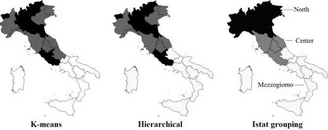
Figure 2: Graphical Representation of the Italian Regions Considering K-Means, Hierarchical Clusters, and Comparison with the Istat Groups (Each Color Represents a

Cluster)

Source: Authors’ elaboration based on Istat data.

The hierarchical clusters appear less defined in the considered period2 because some regions of central Italy are not clearly divided into the groups of the Center-North and the South. For this problem, we consider the k-means divisions as the most appropriate. Figure 2 represents the abovementioned cluster divisions for a better representation of the possible groups of regions. We note that the two cluster techniques suggest the same two groups, formed by the geographical central and northern regions (black and gray regions). Considering these groups and the GDP per capita values (Table 2), the white regions in the k-means map constitute the relatively poor “South” and are approximately in the official Mezzogiorno area (compare with the right map). We consider the other two groups as both representatives of the wealthiest macro area. The black regions in the k-means map (hereinafter Center-North 1) are those with a higher income and the greatest economic development and include the cities of Rome and Milan. In the gray regions (hereinafter Center-North 2), manufacturing firms play the most important role because of the widespread presence of small and medium enterprises.

Furthermore, this grouping allows us to increase the comparability of data for economic homogeneity and the numbers of the population involved. In fact, the Center-North 1 has a population of 21,529,780; Center-North 2 has 18,360,660 inhabitants, and the South group has 19,573,598 inhabitants3 (in 2015, on Istat data).

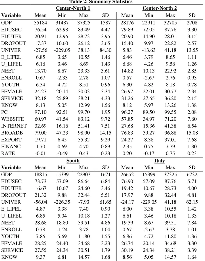
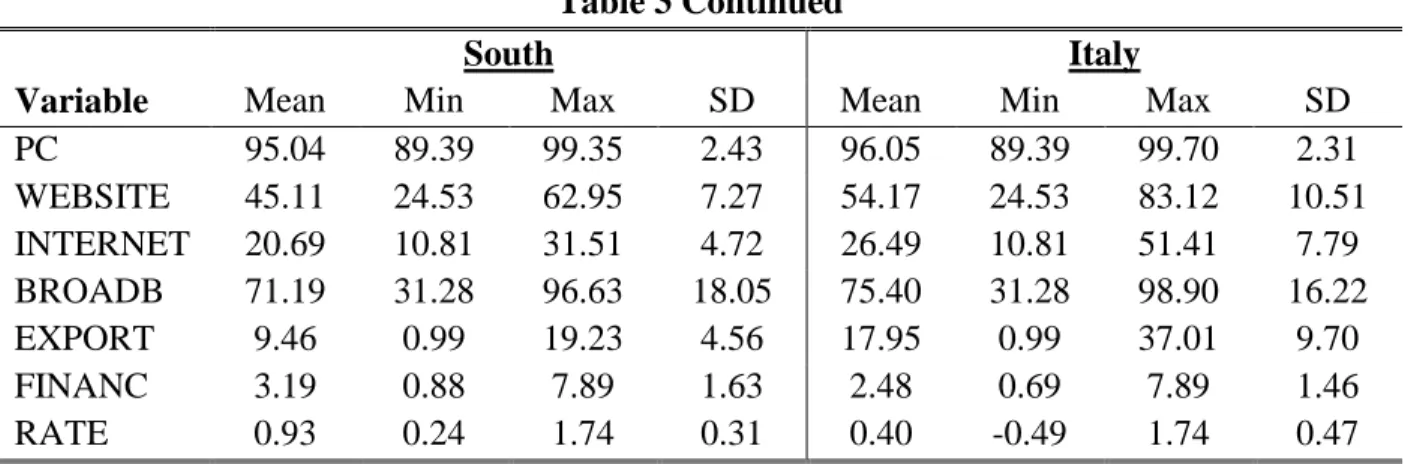
After grouping the regions, Table 3 reports the statistical summary of the variables considered for the three groups and for Italy. We observe similar educational values in all regions, while the aspects that negatively affect human capital are different (high NEET and dropout rates in the South). Differences are also present in the business-specific variables because of the different level of economic development, and this is reflected in the export values. Obviously, a series of local inefficiencies also causes negative consequences that are synthetically illustrated by

2_{As the analysis covers 10 years, in a few cases, regions spend 5 years in two different clusters; in these cases, we have included} the region in the cluster according to the other clustering technique.

(12)

financial data in the South, distant from the national average, and that limit economic growth, or in this case, the economic recovery during a recession.

Table 2: Summary Statistics

Center-North 1 Center-North 2

Variable Mean Min Max SD Mean Min Max SD

GDP 35184 31487 37325 1587 28176 22911 32705 2708 EDUSEC 76.54 62.98 83.49 4.47 79.89 72.05 87.76 3.30 EDUTER 20.91 12.96 28.73 3.95 20.90 14.90 28.01 3.15 DROPOUT 17.37 10.60 26.12 3.65 15.40 9.97 22.82 2.57 UNIVER -27.56 -229.05 38.13 84.30 5.83 -13.63 41.18 13.55 E_LIFEL 6.85 3.65 10.55 1.46 6.46 3.79 8.65 1.11 U_LIFEL 6.16 3.46 8.69 1.43 6.68 4.26 9.56 1.26 NEET 13.70 8.67 23.33 3.61 14.82 10.13 22.92 2.85 ENROLL 0.67 -2.33 2.78 1.07 0.57 -2.67 2.76 0.93 YOUTH 6.34 4.72 8.51 0.96 6.30 4.82 8.18 0.78 FEMALE 24.27 20.14 30.03 3.34 26.97 22.01 30.77 2.34 SERVICE 32.18 25.89 38.21 4.33 31.26 27.65 36.20 2.15 KNOW 8.13 5.05 12.99 1.56 8.12 5.97 13.26 1.38 PC 97.10 92.51 99.70 1.95 96.27 89.50 99.55 2.08 WEBSITE 60.97 41.54 83.12 9.72 57.85 34.97 71.20 7.60 INTERNET 32.69 16.16 51.41 7.51 27.68 15.36 41.38 6.54 BROADB 79.00 47.23 98.90 14.15 76.83 39.27 96.88 15.08 EXPORT 19.71 6.45 35.32 9.29 24.27 8.38 37.01 7.68 FINANC 1.70 0.69 4.70 0.89 2.35 0.75 7.79 1.30 RATE -0.01 -0.49 0.43 0.23 0.20 -0.17 0.75 0.23 South Italy

GDP 18815 15399 22907 1671 26652 15399 37325 6732 EDUSEC 73.73 57.09 86.64 6.84 76.90 57.09 87.76 5.71 EDUTER 16.67 10.67 24.60 3.46 19.42 10.67 28.73 4.00 DROPOUT 21.32 9.88 32.44 5.51 17.97 9.88 32.44 4.81 UNIVER -56.04 -226.35 -7.93 61.65 -24.17 -229.05 41.18 62.15 E_LIFEL 4.87 3.38 7.40 0.90 6.00 3.38 10.55 1.42 U_LIFEL 6.85 5.04 10.18 1.27 6.61 3.46 10.18 1.33 NEET 28.68 18.80 39.51 4.86 19.39 8.67 39.51 7.84 ENROLL 0.78 -1.24 3.78 1.04 0.67 -2.67 3.78 1.01 YOUTH 7.86 5.69 11.80 1.55 6.86 4.72 11.80 1.36 FEMALE 28.25 24.40 34.68 3.23 26.74 20.14 34.68 3.30 SERVICE 27.55 24.34 30.51 1.79 30.19 24.34 38.21 3.39 KNOW 9.37 6.81 14.57 1.68 8.56 5.05 14.57 1.64

(13)

Table 3 Continued

South Italy

PC 95.04 89.39 99.35 2.43 96.05 89.39 99.70 2.31 WEBSITE 45.11 24.53 62.95 7.27 54.17 24.53 83.12 10.51 INTERNET 20.69 10.81 31.51 4.72 26.49 10.81 51.41 7.79 BROADB 71.19 31.28 96.63 18.05 75.40 31.28 98.90 16.22 EXPORT 9.46 0.99 19.23 4.56 17.95 0.99 37.01 9.70 FINANC 3.19 0.88 7.89 1.63 2.48 0.69 7.89 1.46 RATE 0.93 0.24 1.74 0.31 0.40 -0.49 1.74 0.47

Table 3: Summary Statistics for MARS

GDP per capita Center-North 1 Center-North 2 South Italy

Mean (observed) 35183.54 28176.01 18815.34 26651.66

Standard deviation (obs.) 1586.81 2708.21 1671.44 6732.38

Mean (predicted) 35183.54 28176.01 18815.34 26651.66

Standard deviation (predict.) 1571.45 2681.55 1641.67 6595.18

Mean (residual) 0.00 0.00 0.00 0.00

Standard deviation (residual) 220.23 379.09 314.09 1352.20

R2 0.98 0.98 0.96 0.96

R2 adjusted 0.97 0.98 0.96 0.96

GCV 190127.4 378277.6 215702.0 2376237.0

6. MARS AND PANEL DATA ANALYSIS 6.1 MARS Results

We consider all independent variables in the MARS analysis to select the effective determinants of GDP (i.e., those included in the resulting equations) useful in the following step of the analysis. Below, we report in Table 4 the summary results for the MARS models.

In the following, the equations for the groups of regions and for Italy are presented:

GDPCN1 = 31097.32 + 915.16 * max (0; FEMALE - 23.71) + 1270.66 * max (0; 23.71 -

FEMALE) + 149.36 * max (0; EXPORT - 11.76) - 3773.75 * max (0; FINANC - 1.76) - 58.21 * max (0; UNIVER - 14.51) + 2897.57 * max (0; FINANC - 2.05) + 63.94 * max (0; WEBSITE - 59.60) + 97.02 * max (0; 59.60 - WEBSITE) - 547.55 * max (0; 6.29 - YOUTH) - 58.20 * max (0; 78.76 - BROADBAND) + 226.74 * max (0; 18.98 - EDUTER) + 758.10 * max (0; ENROLL - 1.09) GDPCN2 = 26583.02 - 4404.89 * max (0; RATE - 0.07) -2795.87 * max (0; 0.07 - RATE) +

983.91 * max (0; 2.48 - FINANC) + 72.63 * max (0; UNIVER - 0.32) + 168.96 * max (0; 0.32 - UNIVER) - 398.24 * max (0; 32.52 - SERVICE) - 140.81 * max (0; NEET - 13.80) + 597.98 * max

(14)

(0; 13.80 - NEET) + 1921.85 * max (0; FEMALE - 28.99) + 254.42 * max (0; 28.99 - FEMALE) + 61.83 * max (0; EXPORT - 16.38) + 384.95 * max (0; 16.38 - EXPORT) + 108.56 * max (0; 78.34 - EDUSEC) - 1340.25 * max (0; FEMALE - 28.04) -76.33 * max (0; UNIVER - 19.25)

GDPS = 18940.82 - 124.71 * max (0; NEET - 28.23) + 176.74 * max (0; 28.23 - NEET) +

48.04 * max (0; UNIVER + 56.04) + 113.98 * max (0; INTERNET - 24.15) - 346.49 * max (0; 7.90 - U_LIFEL) - 1360.69 * max (0; RATE - 0.79) + 301.04 * max (0; FEMALE - 28.85) - 195.58 * max (0; 93.92 - PC) - 39.27 * max (0; BROADB - 59.29) - 23.73 * max (0; 59.29 - BROADB) - 54.60 * max (0; UNIVER + 22.68)

GDPIT = 15028.59 + 623.30 * max (0; 28.42 - NEET) + 220.77 * max (0; INTERNET -

25.07) - 157.07 * max (0; EDUSEC - 71.33) + 925.28 * max (0; SERVICE - 33.66) - 162.25 * max (0; 33.66 - SERVICE) + 86.07 * max (0; UNIVER - 12.89) + 12.92 * max (0; 12.89 - UNIVER) + 1598.14 * max (0; 2.13 - FINANC) + 4746.39 * max (0; 0.88 - RATE) + 113.47 * max (0; 32.11 - EXPORT) + 788.29 * max (0; 6.50 - U_LIFEL) + 201.88 * max (0; WEBSITE - 66.31)

The observation of the significant variables provides some indications of the local economic specialization. The strength of export is observed in the Center-North, but at the same time, the risk of default of loans slows down the economic recovery. Some ICT indicators seem relevant in the South, even if the difficulty of financing innovation is highlighted by the higher cost of financing rates compared to the rest of the country.

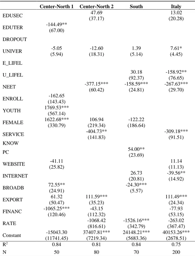
6.2 Fixed Effects Results

We present the results of the fixed effects model (Table 5) for the three groups presented in Section 5. For each group, only the important variables found with MARS are used. The same analysis is carried out for Italy (all regions). The dependent variable is the regional GDP per capita. The results of the three groups show two important aspects that demonstrate the strong effect of the 2007 crisis and the prolonged recession: the importance of credit linked to the businesses’ activities and the lack of attention to human capital. The first aspect is known as a result of the credit crunch issue; the second aspect concerns Italy’s failure to take advantage of the returns from education. For this reason, the relationship between education (and lifelong learning) and GDP is weak (or negative in some regions of the North, see the findings of Di Liberto, 2008), and the relationship may worsen in time of recession.

The industrial tradition is highlighted in the results of the two North-Central groups. Youth and female entrepreneurship are emphasized in the first group, while in the second group, which has an economy focused on manufacturing, the export shows a direct relation, although it is weakened in times of crisis. In fact, foreign trade could be more important because the strength of the manufacturing sector (the most affected by the crisis for Lagravinese, 2015) is hampered by the negative sign of the services for businesses.

Among the southern relevant variables, not enough signs of economic recovery are found and ICT-related indicators of businesses are conflicting. The rate of the young people NEET is a serious problem inducing social distress in all regions in a period of high unemployment, although with large regional differences. This rate is approximately 10–20 percent in the Center-North and 35–40 percent in several southern regions (in the last years of the analysis, via Istat data), and it is linked to the unemployment rate, which is approximately 20 percent in the Mezzogiorno area (8 percent in the North), and to the youth unemployment rate that is over 50 percent (30 percent in the North). These rates are not an encouraging sign for the formation of human capital.

(15)

Table 4: Fixed Effects Model Results for the Three Groups and for Italy

Center-North 1 Center-North 2 South Italy

EDUSEC 47.69 (37.17) 13.02 (20.28) EDUTER -144.49** (67.00) DROPOUT UNIVER -5.05 (5.94) -12.60 (18.31) 1.39 (5.14) 7.61* (4.45) E_LIFEL U_LIFEL 30.18 (92.37) -158.92** (76.65) NEET -377.15*** (60.42) -158.59*** (24.81) -267.63*** (29.70) ENROLL -162.65 (143.43) YOUTH 1769.53*** (567.14) FEMALE 1622.68*** (330.79) 106.94 (219.34) -122.22 (186.64) SERVICE -404.73** (141.83) -309.18*** (91.51) KNOW PC 54.00** (23.69) WEBSITE -41.11 (25.82) 11.14 (11.13) INTERNET 26.73 (20.81) -39.56** (14.92) BROADB 72.55** (24.91) -24.30*** (5.57) EXPORT 61.32 (50.47) 111.59*** (35.23) 111.49*** (24.34) FINANC -1065.25*** (120.46) -43.15 (112.32) -77.93 (53.15) RATE -1068.42 (816.61) -1526.16*** (342.79) -263.02 (367.47) Constant -15043.30 (11741.45) 37407.81*** (7219.34) 24148.21*** (5683.36) 40153.26*** (2678.51) R2 _0.84 _0.81 _0.84 _0.75 N 50 80 70 200

Note: p<0.10*, p<0.05**, p<0.01***. Source: Authors’ elaboration based on Istat data.

Finally, we note that the results of Italy are similar (3 relevant variables out of 6) to the Center-North 2 group, which is also the closest in terms of average GDP per capita. In particular, the importance of export can represent the strength of the recovery after the crisis, but local differences are observed. The NEET problem, linked to high unemployment and the inability to

(16)

leverage business services to increase efficiency and competitiveness, is confirmed at the national level.

7. POLICY IMPLICATIONS AND CONCLUSIONS

Regional economic integration serves to promote the economic and social cohesion for a common development path, and this promotion is confirmed by the fact that a common developmental path is considered among the European Union’s main objectives (Monfort, 2008). The purpose of obtaining a balanced and joint growth has led, for example, to investing over 350 billion euros during the financial programming period 2007–2013, and over 300 billion are planned in the period 2014–2020.4 The European Union (2012) Treaty expresses this concept:

In order to promote its overall harmonious development, the Union shall develop and pursue its actions leading to the strengthening of its economic, social, and territorial cohesion. In particular, the Union shall aim at reducing disparities between the levels of development of the various regions and the backwardness of the least favoured regions.

–EU Treaty, Article 174 (ex Article 158 TEC)

The European efforts have existed for decades, while strong criticisms have been expressed about their effectiveness (see, among others, Sapir et. al., 2004).

Although there are traces of convergence for clubs of regions (De Siano and D’Uva, 2006; Borsi and Metiu, 2013), it is evident from our preliminary analysis that economically backward regions remain on development paths far from the richest areas, showing signs of divergence even within countries. This situation is evident in Italy, and the 2007 crisis, followed by a prolonged recession, has certainly contributed negatively.

The presence of a part of a country less economically developed is a problem that has existed in Italy for decades (Daniele and Malanima, 2011), and there is no evidence that the regional gaps are declining. Italy is a country in which some northern regions have an average income 30 percent higher than the EU average, and several southern regions are 40 percent below. At the national level, the strong inequality causes an average income of the richest area equal to almost double that of the poorest regions of the so-called Mezzogiorno (formed by the geographic South and the major islands).

We analyze the reasons for the growing differences in income by studying the differences in the sources of local wealth. Two preliminary considerations have been made: the usefulness of obtaining clusters of regions referring to the period under study and the opportunity of the implementation of a data mining technique to filter the variables (among 19 regressors) most useful to be analyzed in the local contexts.

The Center-North/South division is evident in our clusters, and it largely confirms the findings of Brida, Garrido, and Mureddu (2014). Furthermore, the gaps in many socioeconomic variables and the different determinants of GDP per capita show ample evidence to the strengthening of the dualism.

(17)

We use a MARS model, a non-parametric technique, to study relations among variables in a large dataset with the objective of obtaining information on the effective factors influencing the regional GDP. The relevant statistical variables depict sources of dualism (e.g., the export strength) but also common problems induced by the prolonged recession (such as the NEET rate and the scarce relevance of human capital).

The variables selected using MARS allow obtaining group-specific results using a fixed effects model. The results confirm the presence of a negative phase of the economic cycle in Italy, which is amplified by the lack of economic recovery that was expected for 2010. The analysis reveals that some local strengths allow a (weak) recovery starting from the relations with foreign markets and promoting new categories of entrepreneurs. These strengths, however, continue to favor only the richest area in the country.

These findings are confirmed in different ways by the comparison of two groups of regions representing the wealthiest Center-North area with the “poor” South. The first group, formed by the wealthiest regions, highlights the importance of young and female entrepreneurship, which are the only categories capable to withstand the crisis and to recover more quickly thanks to their characteristics: multiculturality and predisposition to innovation. This fact is also detected by Unioncamere (2016), the Union of Chambers of Commerce of Italy. The second Center-North group bases its strength on manufacturing enterprises (non-high-tech) and the presence in international markets.

The economic support of human capital, which should be the main economic resource in the knowledge economy era, is absent, confirming the findings of Di Liberto (2008). In the North, this deficiency could be affected by the importance of the manufacturing sector employing untrained workers; in the South, the low-tech specialization induces a higher school dropout (19 percent in 2015, almost double that of the North) and, in some cases, the migration of trained workers (Faggian, Rajbhandari, and Dotzel, 2017). High education and the lifelong learning process are more widespread in the North, while it lacks the capacity to fully exploit this resource.

In summary, the strong industrial development in the North provides adequate growth rates even in times of recession, thanks to the development of local financial systems, despite the inability to properly capitalize on the local human capital. These conditions are lacking in the South, and it is probably not useful to search for industrial convergence in the era of intangible resources. Moreover, under the same conditions, labor productivity in the South seems to be lower, as discussed below.

In general, the human capital role is not properly exploited because of the general low-tech specialization and the lack of understanding of the importance of advanced education (and even more of lifelong learning). This is a missed opportunity of convergence because education is a major factor influencing productivity, and increased productivity is a major source of catch up in Italy (Di Liberto, Pigliaru, and Mura, 2008).

During the years of prolonged recession, credit is another relevant and common aspect involving the North and the South. The risk of credit default is relevant in the wealthiest Center-North group because of non-performing businesses during the recession period. In the southern regions, the indicator of the North-South differential rates shows how the scarce financial resources to provide loans were hampered by higher costs, thus affecting consumption and investment opportunities. In synthesis, the South’s financial structural weaknesses strongly affect

(18)

economic recovery during the recession period, and the increase in the efficiency of local financial systems seems an indispensable condition for spreading new investments.

However, the Italian disparities configure different possible policy responses to the described major economic problems to enhance economic and social integration. A first aspect regards the historical regional differences in Italy, thus inducing the exploitation of the local characteristics of the regions, as contemplated in the discussions on the EU smart specialization strategy (Camagni and Capello, 2013).

Another important aspect that we have observed and that deserves the attention of policy makers regards human capital, which should be considered for a homogeneous and consistent growth path. The scarce relationship between (advanced) education and GDP is a major weakness in all regions, and human capital can represent a possible source of economic recovery in the South and, consequently, of economic convergence. Positive aspects had been observed before the 2007 crisis in the Mezzogiorno (see the “New Regionalism” by Rossi, 2004), although there were strong territorial differences. In addition to a different specialization of businesses, structural changes in society are needed to realize the importance of human capital, and this should lead to the expected economic development instead of further industrialization. In fact, other types of capital are needed to enhance the human capital development as highlighted, for example, by Tabellini on the role of the culture:

Culture is measured by indicators of individual values and beliefs, such as trust and respect for others, and confidence in individual self-determination.

–Tabellini (2010, p. 677).

The different historical paths have caused delays in the southern social capital formation, which is currently one of the causes of the weaker economic development (Putnam, 1993). For example, Felice and Vasta (2015) suggest that there has been a high convergence in life expectancy, incomplete convergence in education, and divergence in GDP among the Italian regions, and the social component has played a key role at the expense of the South.

Despite the well-known differences in cultural, social, and human capital,5_{these are all}

fundamental aspects, and they must co-exist to support economic development. Higher education and lifelong learning need to become the conscious goal of businesses and households. Concerning education, structural weaknesses are found in the South, while only delays due to the recession period are present in the Center-North.

The aforementioned southern weaknesses, because of the South’s history and the wrong decisions of policy makers (Trigilia, 2012), are more evident during times of crisis and are among the major causes of the increasing North-South dualism. The inadequacies, from social to human capital, affect the productivity of workers and businesses, the efficiency of local financial systems, and, consequently, the ability to innovate and export. As mentioned, the data show that these problems add to the difficulty of accessing credit. Investments in education and training, linked to continuous innovation by businesses, seem to be points of strength for returning to growth and to fill, in the long-run, both social and economic gaps with the North.

This article is a first application of the presented method, consisting of several steps of analysis. An interesting development of the research, useful to exploit the capabilities of the

(19)

MARS model, could be to consider a larger dataset or to increase the sample size. A limitation is given by the availability of data, while at least two alternatives exist: considering a lowest administrative grouping (e.g., the provinces in the Italian case) or comparing the regions of more countries.

REFERENCES

A’Hearn, Brian and Anthony J. Venables. (2013) “Regional Disparities: Internal Geography and External Trade,” in Gianni Toniolo, ed., The Oxford Handbook of the Italian Economy

Since Unification. Oxford University Press: Oxford, U.K., pp. 599–630.

Abel, Jaison R., Ishita Dey, and Todd M. Gabe. (2012) “Productivity and the Density of Human Capital,” Journal of Regional Science, 52, 562–586.

Abraham, Ajith, Dan Steinberg, and Ninan Sajeeth Philip. (2001) “Rainfall Forecasting Using Soft Computing Models and Multivariate Adaptive Regression Splines,” IEEE SMC

Transactions - Special Issue on Fusion of Soft Computing and Hard Computing in

Industrial Applications.

Abramo, Giovanni, Ciriaco A. D’Angelo, and Francesco Rosati. (2016) “The North–South Divide in the Italian Higher Education System,” Scientometrics, 109, 2093–2117.

Aghion, Philippe and Peter W. Howitt. (1998) Endogenous Growth Theory. MIT Press: Cambridge, MA.

Alesina, Alberto F., Stephan Danninger, and Massimo Rostagno. (1999) “Redistribution Through Public Employment: The Case of Italy,” IMF WP No. 99/177, International Monetary Fund.

Annoni, Paola and Angél Catalina Rubianes. (2016) “Tree-Based Approaches for Understanding Growth Patterns in the European Regions,” Region, 3, 23–45.

Arbia, Giuseppe and Roberto Basile. (2005) “Spatial Dependence and Non-linearities in Regional Growth Behaviour in Italy,” Statistica, 65, 145–167.

Azzoni, Carlos R. (2001) “Economic Growth and Regional Income Inequality in Brazil,” Annals

of Regional Science, 35, 133–152.

Barro, Robert J. and Xavier Sala-I-Martin. (1991) “Convergence Across States and Regions,”

Brookings Papers on Economic Activity, 22, 107–182.

Benhabib, Jess and Mark M. Spiegel. (1994) “The Role of Human Capital in Economic Development: Evidence from Aggregate Cross-country Data,” Journal of Monetary

Economics, 34, 143–173.

Borsi, Mihály T. and Norbert Metiu. (2013) “The Evolution of Economic Convergence in the European Union,” Deutsche Bundesbank Discussion Paper No. 28/2013.

Bowlus, Audra J. and Chris Robinson. (2012) “Human Capital Prices, Productivity, and Growth,”

American Economic Review, 102, 3483–3515.

Breton, Theodore R. (2013) “Were Mankiw, Romer, and Weil Right? A Reconciliation of the Micro and Macro Effects of Schooling on Income,” Macroeconomic Dynamics, 17, 1023– 1054.

(20)

Brida, Juan G., Nicolás Garrido, and Francesco Mureddu. (2014) “Italian Economic Dualism and Convergence Clubs at Regional Level,” Quality & Quantity, 48, 439–456.

Camagni, Roberto and Roberta Capello. (2013) “Regional Innovation Patterns and the EU Regional Policy Reform: Toward Smart Innovation Policies,” Growth and Change, 44, 355–389.

Capello, Roberta. (2016) “What Makes Southern Italy Still Lagging Behind? A Diachronic Perspective of Theories and Approaches,” European Planning Studies, 24, 668–686. Caselli, Francesco and Wilbur J. Coleman II. (2001) “The U.S. Structural Transformation and

Regional Convergence: A Reinterpretation,” Journal of Political Economy, 109, 584–616. Chen, Shu-Heng, Hung-Wen Lin, Edgardo Bucciarelli, Fabrizio Muratore, and Iacopo Odoardi. (2018) “A Data Mining Analysis of the Chinese Inland-Coastal Inequality,” in Edgardo Bucciarelli, Shu-Heng Chen, and Juan M. Corchado, eds., Decision Economics. Springer: Cham, pp. 96–104.

Dall’Erba, Sandy and Fang Fang. (2015) “Meta-Analysis of the Impact of European Union Structural Funds on Regional Growth,” Regional Studies, 51, 822–832.

Daniele, Vittorio and Paolo Malanima. (2007) “Il Prodotto delle Regioni e il Divario Nord-Sud in Italia 1861–2004,” Journal of Economic Policy, 97, 267–316.

_____. (2011) Il Divario Nord-Sud in Italia 1861–2011. Rubbettino: Soveria Mannelli.

De Graaf, Nan D., Paul M. De Graaf, and Gerbert Kraaykamp. (2000) “Parental Cultural Capital and Educational Attainment in the Netherlands: A Refinement of the Cultural Capital Perspective,” Sociology of Education, 73, 92–111.

De Siano, Rita and Marcello D’Uva. (2006) “Club Convergence in European Regions,” Applied

Economics Letters, 13, 569–574.

Deichmann, Joel, Abdolreza Eshghi, Dominique Haughton, Selin Sayek, and Nicholas Teebagy. (2002) “Application of Multiple Adaptive Regression Splines (MARS) in Direct Response Modeling,” Journal of Interactive Marketing, 16, 15–27.

Démurger, Sylvie. (2001) “Infrastructure Development and Economic Growth: An Explanation for Regional Disparities in China?,” Journal of Comparative Economics, 29, 95–117. Di Liberto, Adriana, Francesco Pigliaru, and Roberto Mura. (2008) “How to Measure the

Unobservable: A Panel Technique for the Analysis of TFP Convergence,” Oxford

Economic Papers, 60, 343–368.

Di Liberto, Adriana. (2008) “Education and Italian Regional Development,” Economics of

Education Review, 27, 94–107.

Dunford, Mick. (1995) “Metropolitan Polarization, the North-South Divide, and Socio-Spatial Inequality in Britain: A Long-Term Perspective,” European Urban and Regional Studies, 2, 145–170.

Durlauf, Steven N. (2009) “The Rise and Fall of Cross-Country Growth Regressions,” History of

Political Economy, 41, 315–333.

Edwards, Richard, Stewart Ranson, and Michael Strain. (2002) “Reflexivity: Towards a Theory of Lifelong Learning,” International Journal of Lifelong Education, 21, 525–536.

(21)

Elhorst, J. Paul. (2014) “Spatial Panel Data Models,” in J. Paul Elhorst, ed., Spatial Econometrics. Springer-Verlag: Berlin Heidelberg, 37–93.

Ertur, Cem, Julie Le Gallo, and Catherine Baumont. (2006) “The European Regional Convergence Process, 1980–1995: Do Spatial Regimes and Spatial Dependence Matter?,” International

Regional Science Review, 29, 3–34.

Etzo, Ivan. (2011) “The Determinants of the Recent Interregional Migration Flows in Italy: A Panel Data Analysis,” Journal of Regional Science, 51, 948–966.

European Union. (2012) “Consolidated Version of the Treaty on the Functioning of the European Union,” Official Journal of the European Union C 326, 55, 47–199.

Faggian, Alessandra, Isha Rajbhandari, and Kathryn R. Dotzel. (2017) “The Interregional Migration of Human Capital and Its Regional Consequences: A Review,” Regional Studies, 51, 128–143.

Faini, Riccardo, Giampaolo Galli, Pietro Gennari, and Fulvio Rossi. (1997) “An Empirical Puzzle: Falling Migration and Growing Unemployment Differentials Among Italian Regions,”

European Economic Review, 41, 571–579.

Fargion, Valeria. (1996) “Social Assistance and the North–South Cleavage in Italy,” South

European Society and Politics, 1, 135–154.

Fattahi, Shahram. (2011) “A Comparative Study of Parametric and Nonparametric Regressions,”

Iranian Economic Review, 16, 19–43.

Felice, Emanuele. (2007) Divari Regionali e Intervento Pubblico: Per una Rilettura dello Sviluppo

in Italia. Il Mulino: Bologna.

Felice, Emanuele and Michelangelo Vasta. (2015) “Passive Modernization? The New Human Development Index and Its Components in Italy’s Regions (1871–2007),” European

Review of Economic History, 19, 44–66.

Felicisimo, Ángel M., Aurora Cuartero, Juan Remondo, and Elia Quirós. (2013) “Mapping Landslide Susceptibility with Logistic Regression, Multiple Adaptive Regression Splines, Classification and Regression Trees, and Maximum Entropy Methods: A Comparative Study,” Landslides, 10, 175–189.

Ferri, Giovanni and Marcello Messori. (2000) “Bank–Firm Relationships and Allocative Efficiency in Northeastern and Central Italy and in the South,” Journal of Banking &

Finance, 24, 1067–1095.

Fitzmaurice, Garrett M., Nan M. Laird, and James H. Ware. (2004) Applied Longitudinal Analysis. John Wiley & Sons: Hoboken, NJ.

Fleisher, Belton, Haizheng Li, and Min Qiang Zhao. (2010) “Human Capital, Economic Growth, and Regional Inequality in China,” Journal of Development Economics, 92, 215–231. Friedman, Jerome H. (1991) “Multivariate Adaptive Regression Splines,” Annals of Statistics, 19,

1–67.

_____. (1993) “Fast MARS,” Department of Statistics - Stanford University Technical Report No.

(22)

Gennaioli, Nicola, Rafael La Porta, Florencio Lopez-de-Silanes, and Andrei Shleifer. (2013) “Human Capital and Regional Development,” Quarterly Journal of Economics, 128, 105– 164.

Gitto, Simone and Paolo Mancuso. (2015) “The Contribution of Physical and Human Capital Accumulation to Italian Regional Growth: A Nonparametric Perspective,” Journal of

Productivity Analysis, 43, 1–12.

Goldin, Claudia. (2016) “Human Capital,” in Claude Diebolt and Michael Haupert, eds.,

Handbook of Cliometrics. Springer-Verlag: Berlin Heidelberg, pp. 55–86.

Hastie, Trevor, Robert Tibshirani, and Jerome Friedman. (2001) The Elements of Statistical

Learning: Data Mining, Inference and Prediction. Springer-Verlag: New York, NY.

Helliwell, John F. and Robert D. Putnam. (1995) “Economic Growth and Social Capital in Italy,”

Eastern Economic Journal, 21, 295–307.

Hill, Thomas and Pawel Lewicki. (2006) Statistics: Methods and Applications. A Comprehensive

Reference for Science, Industry, and Data Mining. StatSoft: Tulsa, OK.

Imbriani, Cesare, Rosanna Pittiglio, Filippo Reganati, and Edgardo Sica. (2014) “How Much Do Technological Gap, Firm Size, and Regional Characteristics Matter for the Absorptive Capacity of Italian Enterprises?,” International Advances in Economic Research, 20, 57– 72.

Islam, Nazrul. (2003) “What Have We Learned From the Convergence Debate?,” Journal of

Economic Surveys, 17, 309–362.

Jian, Tianlun, Jeffrey D. Sachs, and Andrew M. Warner. (1996) “Trends in Regional Inequality in China,” China Economic Review, 7, 1–21.

Lagravinese, Raffaele. (2015) “Economic Crisis and Rising Gaps North-South: Evidence from the Italian Regions,” Cambridge Journal of Regions, Economy, and Society, 8, 331–342. Lee, Jin Man and Jin Wook Choi. (2011) “The Role of House Flippers in a Boom and Bust Real

Estate Market,” Journal of Economic Asymmetries, 8, 91–109.

Lee, Tian-Shyug, Chih-Chou Chiu, Yu-Chao Chou, and Chi-Jie Lu. (2006) “Mining the Customer Credit Using Classification and Regression Tree and Multivariate Adaptive Regression Splines,” Computational Statistics & Data Analysis, 50, 1113–1130.

Levine, David I. (1998) Working in the Twenty-First Century: Policies for Economic Growth

Through Training, Opportunity, and Education. M. E. Sharpe: Armonk, NY.

Li, Guangdong and Chuanglin Fang. (2014) “Analyzing the Multi-Mechanism of Regional Inequality in China,” Annals of Regional Science, 52, 155–182.

Lin, Pei-Chien, Chun-Hung Lin, and I-Ling Ho. (2013) “Regional Convergence or Divergence in China? Evidence from Unit Root Tests with Breaks,” Annals of Regional Science, 50, 223– 243.

Mankiw, Gregory N., David Romer, and David N. Weil. (1992) “A Contribution to the Empirics of Economic Growth,” Quarterly Journal of Economics, 107, 407–437.

Martin, Ron. (1988) “The Political Economy of Britain’s North-South Divide,” Transactions of

(23)

Mina, Christian D. and Erniel B. Barrios. (2010) “Profiling Poverty with Multivariate Adaptive Regression Splines,” Philippine Journal of Development, 37, 55–97.

Monfort, Philippe. (2008) “Convergence of EU Regions - Measures and Evolution,” European

Union Regional Policy WP 01/2008.

Odoardi, Iacopo, Fabrizio Muratore, Edgardo Bucciarelli, and Shu-Heng Chen. (2018) “Looking for Regional Convergence: Evidence from the Italian Case with Multivariate Adaptive Regression Splines,” in Edgardo Bucciarelli, Shu-Heng Chen, and Juan M. Corchado, eds.,

Decision Economics. Springer: Cham, pp. 77–85.

Ozgen, Ceren, Peter Nijkamp, and Jacques Poot. (2010) “The Effect of Migration on Income Growth and Convergence: Meta-Analytic Evidence,” Papers in Regional Science, 89, 537– 561.

Pedroni, Peter and James Yudong Yao. (2006) “Regional Income Divergence in China,” Journal

of Asian Economics, 17, 294–315.

Putnam, Robert D. (1993) Making Democracy Work: Civic Traditions in Modern Italy. Princeton University Press: Princeton, NJ.

Ramos, Raul, Jordi Suriñach, and Manuel Artís. (2010) “Human Capital Spillovers, Productivity and Regional Convergence in Spain,” Papers in Regional Science, 89, 435–447.

Rose, Elaina. (2001) “Ex Ante and Ex Post Labor Supply Response to Risk in a Low-Income Area,” Journal of Development Economics, 64, 371–388.

Rossi, Ugo. (2004) “New Regionalism Contested: Some Remarks in Light of the Case of the Mezzogiorno of Italy,” International Journal of Urban and Regional Research, 28, 466– 476.

Sapir, André, Philippe Aghion, Giuseppe Bertola, Martin Hellwig, Jean Pisani-Ferry, Dariusz Rosati, José Viñals, Helen Wallace, Marco Buti, Mario Nava, and Peter M. Smith. (2004)

An Agenda for a Growing Europe: The Sapir Report. Oxford University Press: Oxford,

U.K.

Tabellini, Guido. (2010) “Culture and Institutions: Economic Development in the Regions of Europe,” Journal of the European Economic Association, 8, 677–716.

Terrasi, Marinella. (1999) “Convergence and Divergence Across Italian Regions,” Annals of

Regional Science, 33, 491–510.

Thompson, Jennifer J., Evan Conaway, and Erin L. Dolan. (2016) “Undergraduate Students’ Development of Social, Cultural, and Human Capital in a Networked Research Experience,” Cultural Studies of Science Education, 11, 959–990.

Throsby, David. (1999) “Cultural Capital,” Journal of Cultural Economics, 23, 3–12.

Trigilia, Carlo. (2012) Non c’è Nord Senza Sud. Perché la Crescita dell’Italia si Decide nel

Mezzogiorno. Il Mulino: Bologna.

Tsionas, Efthymios G. (2000) “Regional Growth and Convergence: Evidence from the United States,” Regional Studies, 34, 231–238.

Unioncamere. (2016) Impresa in Genere - 3° Rapporto Nazionale Sull’Imprenditoria Femminile. Chambers of Commerce of Italy.

(24)

Van Stel, André, Martin Carree, and Roy Thurik. (2005) “The Effect of Entrepreneurial Activity on National Economic Growth,” Small Business Economics, 24, 311–321.

Varian, Hal R. (2014) “Big Data: New Tricks for Econometrics,” Journal of Economic

Perspectives, 28, 3–28.

Von Lyncker, Konrad and Rasmus Thoennessen. (2017) “Regional Club Convergence in the EU: Evidence from a Panel Data Analysis,” Empirical Economics, 52, 525–553.

Williamson, Jeffrey G. (1965) “Regional Inequality and the Process of National Development: A Description of the Patterns,” Economic Development and Cultural Change, 13, 1–84. Zareipour, Hamidreza, Kankar Bhattacharya, and Claudio A. Canizares. (2006) “Forecasting the

Hourly Ontario Energy Price by Multivariate Adaptive Regression Splines,” 2006 IEEE Power Engineering Society General Meeting, Montreal, Quebec.