Università degli Studi di Ferrara
DOTTORATO DI RICERCA IN
Matematica e Informatica
CICLO XVIII
COORDINATORE Prof. Massimiliano Mella
Region-of-interest CT problem:
effective forward operator and
iterative shearlet-based regularization
Settore Scientifico Disciplinare MAT/08
Dottorando
Dott. Bubba Tatiana Alessandra
Tutore
Prof. Zanghirati Gaetano
Abstract
Region-of-interest Computed Tomography (ROI CT) is an X-ray based incomplete data imaging acquisition mode. Currently, it is among the “hot topics” in the field of ray tomographic imaging, due to its potential to lower exposure to X-ray radiation and to reduce the scanning time. This is particularly appealing, especially for the medical imaging community, due to a wide range of applications in biomedical imaging, such as contrast-enhanced cardiac imaging or positioning of intracranial stents.
However, this problem is rather challenging because of the truncation of pro-jections, i.e., of the acquired data. CT is in general an ill-posed problem, and the ill-posedness becomes severe due to incompleteness of the ROI CT dataset, even more as the ROI size gets smaller. Therefore, one of the major issues is that tra-ditional or naive local reconstruction algorithms may be very unstable and might produce unreliable reconstructions, when applied directly to incomplete data, set-ting missing projections to zero. So far, both ad hoc analytic formulae and iterative numerical schemes have been proposed in the literature to address this problem, but typically rely on restrictive assumptions.
This thesis addresses the connection of the reconstruction problem and the incompleteness of the ROI CT data. The main goal is to obtain a stable and feasible reconstruction, possibly under reliable noise circumstances, and without any assumptions either on the size or on the location of the ROI. This would be impossible due to non-uniqueness of the interior problem.
To this end, we formulate the ROI CT reconstruction problem as a convex optimization problem with different regularization levels. A regularized functional based on shearlets, a new multiscale method whose main features are relevant in CT-like applications, is possibly coupled with a Total Variation regularization term. Both a smooth and a nonsmooth version of this convex problem are inves-tigated.
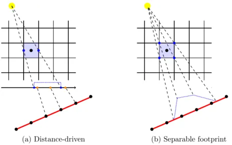
An accurate and flexible forward projection technique, called distance-driven, is considered to study the problem, and an efficient implementation is developed to provide a faster digital reconstruction framework. This original contribution goes beyond the ROI CT problem and applies to more general CT problems.
Two iterative approaches are proposed and analyzed to face the numerical so-lution of the derived convex optimization problem. A scaled gradient projection method for the smooth approach and a variable metric inexact line-search algo-rithm for the nonsmooth case. Both methods have been proposed very recently, and, to the best of our knowledge, it is the first time that their performance is investigated in CT-like applications.
All experimental studies presented make use of simulated data, in the case of 2D fan-beam CT. The numerical tests illustrated in this thesis show that our approach is insensitive to the location of the ROI and remains very stable also when the ROI size is rather small.
The findings and conclusions of this work have a number of important impli-cations for future research. Therefore, suggestions for further work will be given for each addressed topic.
Sommario
La tecnica di Tomografia Computerizzata ristretta a regioni-di-interesse (ROI CT) rientra tra le modalità di acquisizione di immagini tomografiche, mediante raggi X, da dati incompleti. Attualmente, è tra i “temi caldi” nel campo dell’imaging tomografico, poiché offre al contempo la possibiltà di diminuire l’esposizione a radiazioni derivanti dai raggi X e ridurre il tempo di scansione. Per la comunità medica, ROI CT riveste un ruolo di particolare interesse, grazie al gran numero di applicazioni in imaging biomedico, tra cui l’imaging cardiaco con intensificazione di contrasto e il posizionamento di stent intracranici.
Tuttavia, si tratta di un problema piuttosto difficile a causa del troncamento delle proiezioni, cioè dei dati acquisiti. CT è in generale un problema mal posto e, a causa dell’incompletezza dei dati, la mal posizione tende a peggiorare, sem-pre più con il diminuire della dimensione della regione-di-interesse. Perciò, uno dei principali problemi è che gli algoritmi classici o ricostruzioni locali naive pos-sono rivelarsi estremamente instabili, restituendo ricostruzioni inaffidabili, quando applicati ai dati incompleti, ponendo a zero le proiezioni mancanti. A oggi, per affrontare questo problema, sono stati proposti in letteratura sia formule analitiche ad hoc sia schemi numerici iterativi, ma tipicamente si basano su ipotesi restrittive. Questa tesi si propone di investigare la connessione tra il problema di ri-costruzione e l’incompletezza dei dati derivanti dal problema ROI CT. L’obiettivo principale è di ottenere una ricostruzione stabile e ammissibile, possibilmente sotto ipotesi realistiche per il rumore e senza nessun tipo di ipotesi sulla dimensione o posizione della ROI. Ciò sarebbe impossibile a causa della non-unicità dell’interior problem.
A tal fine, ROI CT viene formulato come problema convesso di ottimizzazione, con diversi livelli di regolarizzazione. Si considera un funzionale di regolarizzazione basato sulle shearlets, un metodo multiscala introdotto di recente le cui caratteris-tiche sono rilevanti in applicazioni tomografiche, eventualmente combinato con un termine di tipo Variazione Totale. Di questo problema convesso vengono investi-gate sia una versione differenziabile sia una non differenziabile.
Per lo studio del problema, viene considerata una tecnica accurata e flessibile per la proiezione in avanti, chiamata distance-driven, per la quale è stata sviluppata
un’implementazione efficiente in grado di fornire un ambiente di ricostruzione più veloce. Si tratta di un contributo originale che va al di là del solo problema ROI CT e si applica in generale a tutti i problemi di tipo CT.
Per la soluzione numerica del problema convesso di ottimizzazione vengono proposti e analizzati due approcci iterativi. Per la formulazione differenziabile viene considerato il metodo del gradiente scalato proiettato, mentre per la versione non differenziabile si considera l’algoritmo a metrica variabile inesatta con ricerca in linea. Entrambi i metodi sono stati proposti molto recentemente e, per quanto si è a conoscenza, è la prima volta che queste tecniche vengono investigate in applicazioni di tipo CT.
Tutti gli studi sperimentali che vengono presentati fanno uso di dati simulati nel caso della geometria 2D a ventaglio. I test numerici che vengono illustrati nella tesi mostrano che l’approccio presentato non è influenzato dalla posizione della ROI e rimane molto stabile anche quando la dimensione della ROI è piuttosto piccola.
I risultati e le conclusione di questo lavoro hanno importanti implicazioni per le ricerche future: per ciascun argomento trattato verranno dati spunti per il lavoro futuro.
Acronyms
1D 1-dimensional
2D 2-dimensional
3D 3-dimensional
ART algebraic reconstruction technique
BB Barzilai-Borwein (steplength updating rules) CBGP cyclic scaled gradient projection
CPU central processing unit
CT computed tomography DM data mismatch DBP differentiated back-projection EM expectation maximization ES early stopping FBP filtered back-projection
FDK Feldkamp, Davis, and Kress algorithm FOV field of view
GB gigabyte
GHz gigahertz
GPU graphics processing unit
IRR iterative reconstruction-reprojection
LS least square
LSCG LS conjugate gradient
MAP maximum a posteriori
MART multiplicative ART
MBIR model-based iterative reconstruction
ML maximum likelihood
ML-EM maximum likelihood expectation-maximization MRA multiresolution analysis
MRI magnetic resonance imaging NDT nondestructive material testing
OS ordered subsets
PET positron emission tomography v
PSNR peak-signal-to-noise ratio ROI region-of-interest
ROI CT region-of-interest tomography
SART simultaneous ART
SIRT simultaneous iterative reconstruction technique SGP scaled gradient projection (method)
SPECT single photon emission computed tomography SVD singular values decomposition
TB terabyte
TV total variation
Symbols
⊗ Kronecker product ⟨·, ·⟩ inner product in Rn ⌈·⌉ ceil function ⌊·⌋ floor function ∥ · ∥p p-norm in Lp∥ · ∥D norm induced by the symmetric positive definite matrix D
ˆ
g Fourier transform of the function g
0n n-dimensional zero vector
On n-dimensional zero matrix
1n n-dimensional all-ones vector
1A characteristic function of the set A
1n n-dimensional identity matrix
R+ set of positive real number (not including zero) R− set of negative real number (including zero)
R+0 set of positive real number (including zero)
R∗ set of real number (not including zero)
Zn n-dimensional integer space
Rn n-dimensional euclidean space
Cn n-dimensional complex space
a scaling parameter (unless otherwise specified)
a = (au, av) detector offset
A generic point on the object – Chapter 3
A set of rotation angles
Aa scaling matrix depending on the scaling parameter a
An n-dimensional full affine group of motions
α steplength (unless otherwise specified)
αk steplength at iteration k
b pixels or voxels basis function for object discretization bi i-th (generic) basis function for object discretization
B2(0, r) 2D euclidean ball centered in 0 with radius r
B∞(0, r) infinity-norm centered in 0 with radius r
B linear operator for proximal inexact computation (VMILA)
β elevation angle of a cone-beam system– Chapter 3
β backtracking parameter – Chapters 5, 6
cx, cy, c1 flags in distance-driven vectorized approach
c(n) vector of the center coordinates of the object voxel n
C isocenter – Chapter 3
C (generic) convex set
Cn
unit cylinder in Rn
C centered cube of the shearlets 3D frequency domain parti-tion
Ci i-th cone of the shearlets 2D frequency domain partition
Cn(·) class of functions differentiable with continuity up to order
n
C∞(·) class of infinitely differentiable functions
C∞
0 (·) C
∞ functions with bounded support
γ aperture angle of a cone-beam system – Chapter 3
γ backtracking parameter – Chapters 5, 6
Γ (generic) objective function
Γ0 smooth part of an objective function Γ
Γ1 nonsmooth part of an objective function Γ
dAB distance ∥B − A∥2 between the points A and B
dS(·) distance from the source – Chapter 3
dσ(·) distance-like function
d descent direction
d(k) descent direction at iteration k
D scaling matrix in SGP and VMILA
Dk scaling matrix at iteration k
DM dilation operator associated to the matrix M
DL compact set of the symmetric positive definite matrices D
with threshold L
D (discrete) derivative approximation for TV definition
δ TV smooth parameter
δ(·) Dirac δ function
δ grid increment vector for detector grid
∆ grid increment for “equilateral” pixel or voxel grid
∆ grid increment vector for object grid
∇ discrete gradient operator
∇i i-block of the discrete gradient operator
en n-th versor of the canonical basis
ix
E cartoon-like images
η parameter of η-approximation (VMILA)
θ angle associated to the direction of the ray, i.e., rotation angle
Θ (generic) low pass operator
ζmin, ζmax lowermost and the uppermost z coordinates of the projec-tions of the endpoints of all the vertical edges of the voxels midway slices
f object (attenuation or density) function
¯
f ML or MAP reconstruction
fJ best J -term approximation (shearlets)
f column vector representing the object to reconstruct (dis-cretization of the attenuation or density function f )
¯
f ML or MAP estimate
f∗ ML or MAP solution
f(k) ML or MAP estimate at iteration k
F analysis operator
F∗ synthesis operator
ϕ scaling function
φi element of a frame sequence
Φ shearlet matrix in ROI CT objective function formulation
ΦT transpose of the matrix Φ
ψ mother wavelet or shearlet
ψa,t element of a 1D continuous wavelet system
ψj,m element of a 1D discrete wavelet system
ψM,t element of a nD wavelet system
ψLM Lemariè-Meyer wavelet
ψa,s,t element of a 2D shearlet system
ψj,k,m element of a 2D discrete shearlet system
ψMa,s,t element of a nD shearlet system
g (generic) measured data
gσ (generic) noisy measured data
g∗ conjugate function of a (generic) function g gLL
i , gRLi , gLRi , gRRi column vectors containing all the overlap differences
hσ(·) function that defines the primal variable in VMILA
hH,i column vector containing all the horizontal overlaps hV,j column vector containing all the vertical overlaps
hH,i,1, hH,i,2, hH,i,3 column vector containing the horizontal overlaps corre-sponding to pH,i,1, pH,i,2, pH,i,3, respectively
Hdtc scaling matrix for detector reference system
Hσ(·) dual formulation corresponding to hσ(·) (VMILA)
H (generic) Hilbert space
istart, iinc integers for handling “reversed ordering” in distance-driven
vectorized approach
I identity operator (unless otherwise specified)
I (generic) indices set
Ixz set of rotation angles for which πprj= Oxz
Iyz set of rotation angles for which πprj= Oyz
IvxlH,i indices set for horizontal overlap computation
Ivxl,btmH,i elements of pH,i identifying the voxels slices vertices projec-tions, belonging to the lowest level
IvxlH,i,1, IvxlH,i,2, IvxlH,i,3 indices set for overlap computation, subsets of IvxlH,i Ivxlprj indices set of all voxel projections
Ibtm,sH,idx,i indices of rows in the s-th column of ZH,i whose
correspond-ing z coordinate of midway slices voxel projection is greater than the z coordinate of the projection of the detector bot-tom edge
Itop,sH,idx,i indices of rows in the s-th column of ZH,i whose
correspond-ing z coordinate of midway slices voxel projection is not greater than the z coordinate of the projection of the de-tector top edge
Iαf Riesz potential
ιA indicator function of the set A
k index for third dimension – Chapter 3
k discrete (sampling for the) shearing parameter – Chapter 4
k iteration – Chapters 5, 6
κ memory for the nonmonotone line search
K (generic) linear continuous operator between Hilbert spaces K system matrix, i.e., discretization of an operator K
l dual iteration – Chapters 5, 6
ℓ angle index – Chapter 3
ℓ(θ, τ ) ray at angle θ and with signed distance τ
L detector reference point – Chapter 3
L threshold for the set DL – Chapters 5, 6
LY
y(·) likelihood function
Lmax maximum pixel value
L1(Rn) space of Lebesgue integrable functions on Rn
xi λmin, λmax lowermost and the uppermost z coordinates of the
projec-tions of the detector cells vertical edges endpoints Λ discrete sampling set for irregular shearlet systems m = (mu, mv) number of detector discretization pixels
M mask identifying the ROI
M matrix discretization of the mask M
µ regularization parameter
µk regularization parameter at iteration k
µopt optimal regularization parameter
n n ≥ 1 dimension of the space (unless otherwise specified) n = (nx, ny, nz) number of object discretization voxels
N width and height in pixels of the object to reconstruct
Nθ number of projection angles
Ndtc number of detector cells
Nvxlprj total number of voxels slices vertices to be projected
Nvxl,vrtlyr total number of voxels slices vertices to be projected per
layer N′
vxl extended set of voxels with uppermost virtual layer
ν, νmin, νmax vector containing the detector cells projections for
horizon-tal overlaps computation
O main origin of the inertial system Oxyz
O′ origin of the roto-translated Cartesian system O′utv Oxyz main inertial Cartesian coordinate system
O′utv roto-translated Cartesian coordinate system Ou′t′v′ rototed Cartesian coordinate system
O(·) (implicit or explicit) objective function for ROI CT
Ωf feasible set for f
p norm subscript
pijk linear index position corresponding to vvxl(i, j, k)
˜
pkH displacement of the positions related to the k-th layer pH,leftk , pH,rightk column vectors of the indices of all the leftmost and
right-most endpoints of the horizontal edges of the midway voxel slices projections at layer k
pH,left, pH,right column vectors of the indices of all the leftmost and
right-most endpoints of the horizontal edges of the midway voxel slices projections for all layer
˜
pH displacement vector for the assignment of vertical position to horizontal overlaps
pH,i column vector of the voxel indices whose projections have
a nonempty horizontal overlap with the projections of the i-th column of detector cells
pV,j column vector of the voxel indices whose projections have a
nonempty vertical overlap with the projections of the j-th row of detector cells
pH,i vector of “converted” linear indices (from voxels to voxel vertices)
pH,ibtm column vector corresponding to the indices set Ivxl,btmH,i pH,i,1, pH,i,2, pH,i,3 column vector corresponding to the indices sets
IvxlH,i,1, IvxlH,i,2, IvxlH,i,3, respectively (pH,idx,i min ) s,(p H,idx,i max )
sminimum and maximum row index of the lower voxel in the
s-th stack whose vertical projection reaches the projection of the first cell in the i-th detector column
pH,col,ibtm,s displacement from the global linear index of the voxel at
the bottom of the stack pvxl,H
r column index for WH overlap allocation
pV,low, pV,up column vectors of the indices of all the lowermost and
up-permost endpoints of the vertical edges of the midway voxels slices projections for all layer
pY(·) probability density associated to the random variable Y
pFY joint probability density associated to the random variables
F and Y
pROI ROI center
π(·) unitary representation
πdtc detector plane
πprj common projection plane
P generic point on the detector – Chapter 3
Pη(·) set of η-approximations (VMILA)
PB euclidian projection onto the set B
PB,D scaled euclidian projection onto the set B according to the
scaling matrix D
P(S) ROI-truncated projections
Pi i-th pyramidal region of the shearlets 3D frequency domain
partition
qδ (smooth) approximation of the square root function for TV
definition ˜
qdtc
i rows offset for WH overlap allocation
qdtc
ℓ rows displacement for matrix W
qdtc,i
xiii
ˆ
qH,left,ˆqH,right column vectors of the indices of all the leftmost and right-most endpoints of the detector cells projections for the low-est detector row
qH,left, qH,right column vectors of the indices of all the leftmost and
right-most endpoints of the detector cells projections
qV,low, qV,up column vectors of the indices of all the lowermost and
up-permost endpoints of the vertical edges of the detector cells projections for all layer
rROI ROI radius
Rℓ 2D counter-clockwise rotation matrix of the Oxy
RC(·) cone-beam circular rotation system
Rµ family of operator defining a regularization algorithm
Rf Radon transform of f
R centered square of the shearlets 2D frequency domain par-tition
ρ TV regularization parameter
s shearing parameter (unless otherwise specified)
S region-of-interest (ROI) – Chapters 2, 6
S X-ray source – Chapter 3
S frame operator – Appendix A
Ss shearing matrix depending on the shearing parameter s
Sn−1 unit sphere in Rn
S (Rn)
Schwartz space on Rn
S full shearlet group
SH (continuous and discrete) shearlet system
SH ψ (continuous and discrete) shearlet transform
σH,idx,i
r,s auxiliary vector for horizontal overlap replication
σ noise variance – Chapters 2, 6
σ VMILA set of parameters – Chapter 5
Σ domain of the VMILA set of parameters σ
t translation parameter (usually a vector)
Tt translation operator associated to the (vector) parameter t
T tangent space to the circle
Tn tangent bundle to Sn−1
τi(ℓ) vertical gap for the i-th detector cells vertices column at angle θℓ
τit threshold for stopping iteration in SGP and VMILA
U (·) negative part of the gradient decomposition
U (·) group of unitary operators
˜
v inexact computation of the primal variable v
v(k) primal variable in VMILA at iteration k
˜
v(k,l) inexact computation of v(k)
vvxl(i, j, k) coordinates of a generic object voxel slice in Oxyz
v(ℓ)vxl(i, j, k) coordinates of a generic object voxel slice in Oxyz at angle θℓ
vdtc(i, j) coordinates of a generic detector cell vertice in Oxyz
v(ℓ)dtc(i, j) coordinates of a generic detector cell vertice in Oxyz at angle θℓ
V (·) positive part of the gradient decomposition
Vi(·) i-th component of positive part of the gradient
decomposi-tion
Vvxl set of voxel slices vertices
wm,n distance-driven weights (elements of the matrix W)
w versor of a generic ray
wπprj common projection plane versor
Wψ (continuous and discrete) wavelet transform
WH matrix containing horizontal overlaps
WV matrix containing vertical overlaps
W matrix discretization of the projection geometry
xprj uij, y
prj uij, z
prj
uij projections coordinates of the detector cells vertices vdtc
xprjdtc,0, yprjdtc,0, zprjdtc,0 vectors of the projections of all the detector vertices at layer 0
xprjdtc, yprjdtc, zprjdtc vectors of the projections of all the detector vertices xprj
xijk, y
prj yijk, z
prj
zijk projections coordinates of a single vertex of any voxel slices
xprjvxl,k, xprjvxl,k, xprjvxl,k vectors of the projections of all midway slices vertices at layer k
xprjvxl, xprjvxl, xprjvxl vectors of the projections of all midway slices vertices xi vector representing the i-th basis function center for object
discretization
X f X-ray transform of f
X∗
adjoint operator of X
ξ, ξmin, ξmax vector containing the midway slices projections for horizon-tal overlaps computation
y full sinogram
y0 truncated sinogram
y column vector representing the full sinogram discretization ¯
y ML or MAP estimate of the full sinogram
xv y0 column vector representing the discretization of the
trun-cated sinogram
Y vector valued random variable corresponding to a vector y of measured data (e.g., sinogram)
υ generalized solution of the problem – Chapter 2
υ dual variable in VMILA – Chapters 5, 6
υ(l) dual variable at iteration l
Υ (generic) objective function
Υp Morozov formulation for the ROI CT objective function
ΥDM (generic) data mismatch functional
ΥR (generic) regularization functional
zvxl,minprj , zprjvxl,max minimum and maximum over all z coordinates of the voxels slices projections onto πprj
zdtc,minprj , zdtc,maxprj minimum and maximum over all z coordinates of the detec-tor cells projections onto πprj
ZH,i matrix whose columns contain the vertical coordinates of
the voxels slices vertices projections with linear index in IvxlH,i
Zidx
H,i matrix of integers containing the row indices for the i-th
detector cells column, corresponding to the vertical coordi-nates in ZH,i
Contents
1 Introduction 1
1.1 A brief historical overview . . . 2
1.2 The mathematical viewpoint . . . 3
1.3 Limited data tomography problems . . . 6
1.4 Inverse problems . . . 8
1.5 Thesis outline and original contributions . . . 10
2 Region-of-interest tomography 13 2.1 State-of-the-art . . . 13
2.2 From CT to ROI CT: continuous setup . . . 15
2.2.1 A unique solution for the ROI CT problem . . . 16
2.3 Discrete framework . . . 22
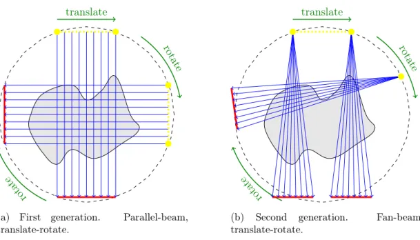
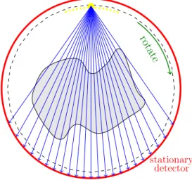
3 Distance-driven vectorized computation 27 3.1 Generations of CT scanners . . . 27
3.2 Object discretization by means of series expansion . . . 31
3.3 State-of-the-art approaches for forward operator . . . 32
3.3.1 The distance-driven technique . . . 35
3.4 Vectorization of the distance-driven technique . . . 36
3.4.1 Cone-beam 3D circular geometry . . . 37
3.4.2 3D vectorized generation of the distance-driven projection matrix . . . 46
4 Shearlets 93 4.1 From wavelets to shearlets . . . 93
4.1.1 One-dimensional continuous wavelet transform . . . 94
4.1.2 Higher-dimensional continuous wavelet transform . . . 97
4.2 Continuous shearlet systems . . . 99
4.2.1 The full shearlet group . . . 103
4.2.2 Cone-adapted and pyramid-based continuous shearlet systems107 4.3 Discrete shearlet systems . . . 112
4.3.1 Regular discrete shearlet systems . . . 112
4.3.2 Cone- and pyramid-adapted discrete shearlet systems . . . . 114
4.3.3 Optimally sparse approximations . . . 118
4.4 Implementation and softwares . . . 120
5 Iterative techniques for ROI CT 121 5.1 Statistical approach for image reconstructions . . . 121
5.2 Scaled gradient projection method . . . 125
5.2.1 Practical implementation of SGP to the ROI CT problem . . 129
5.3 Variable metric inexact line-search algorithm . . . 132
5.3.1 Practical implementation of VMILA to the ROI CT problem 140 6 Numerical experiments 143 6.1 Data simulation . . . 143
6.2 SGP: smooth objective function . . . 147
6.2.1 Implicit formulation . . . 148
6.2.2 Explicit formulation . . . 153
6.2.3 Final Remarks . . . 160
6.3 VMILA: nonsmooth objective function . . . 160
6.3.1 Implicit formulation . . . 160
6.4 Discussion . . . 164
7 Conclusions 173 A Background material on harmonic analysis 177 A.1 Frame Theory . . . 177
A.2 Representation of locally compact groups . . . 180
Bibliography 183
Chapter 1
Introduction
Computed tomography (CT) was historically the first method to allow the possi-bility to acquire images of the inner structure of an object non-invasively, namely without penetrating or cutting into pieces the object. CT has been a major break-through in diagnostic medicine, where, thanks to a non-biased superposition of anatomical features, the internal structures of the human body could be seen dis-tinctly. This opened new opportunities in the recognition and understanding of human diseases without exploratory surgery. Nowadays, CT is used routinely in medicine for diagnostic purpose, thanks to the clarity and accuracy of images pro-duced by CT scanners. Although magnetic resonance imaging (MRI) and positron emission tomography (PET) have been widely installed in worldwide medicine de-partments, CT is, to date, the most widely used imaging diagnostic device in hospital departments and trauma clinic [23].
However, the revolution brought by CT does not end with radiology and nuclear medicine. In fact, the very first application of CT in 1956 took place in radio astronomy, and was due to Ronald Bracewell [20]. Later on, diverse technical, anthropomorphic, forensic, archeological, as well as paleontological, applications of CT have been developed [23]. The underneath leitmotif is to provide a generic industrial diagnostic tool for nondestructive material testing (NDT).
Up to date, it has been about 130 years, counting from the discovery of X-rays by Wilhelm C. Röntgen in 1895, of active research in the field of X-ray tomographic imaging. Nevertheless, research in the field of CT is still as exciting as at the beginning of its development during the 1960s and 1970s.
The focus of this thesis is region-of-interest tomography (ROI CT), a limited data tomographic acquisition mode, that will be described in Section 1.3. After a long period, from the late 1970s to the early 1990s, during which the ROI CT problem was believed to be insolvable, the intensive research in the last decade not only revealed the reconstruction from incomplete data possible but also counted ROI CT in the “hot topics” in the field of X-ray tomographic imaging [33]. The
primary interest lays in the possibility to reduce the scanning time and lower the X-ray radiation dose, while maintaining the possibility to handle large object, in high resolution.
1.1
A brief historical overview
The history of X-ray imaging starts in 1895 with the discovery of a new kind of radiation called “X-rays” by its finder Wilhelm C. Röntgen. Between 1895-1896 Röntgen conducted a series of experiments to show that there existed, indeed, a technique able to take “X-ray photographs” of the internal features of a person without any surgical intervention [141, 140]. Quickly, his technique found justified recognition among doctors and spread worldwide: for this, he was awarded the Nobel prize in 1901.
By the 1930s, the design of X-ray equipment was refined. Simple radiographs of early attempts contained the 2D shadow deriving from the superposition of all 3D structures in the object. Thus, it was impossible to recover precise informations concerning any particular feature of interest. At the beginning of the 1920s, there were many attempts to erase superimposed shadows from X-ray images. The goal was to display sharply the plane in focus and to blur the out of focus planes. This resulted in a number of patent applications (e.g., A.E.M. Bocage in 1922 [12] and E. Pohl in 1927 [133]) and a number of papers published by researchers from different countries that were rediscovering similar concepts: all those works dealt with the same geometry technique, in which the X-ray tube and the detector moved along two parallel planes. As a consequence, the technique became known under several names: it was called stratigrafia by A. Vallebona [153], laminography by J. Kieffer [93] and planigraphy by A.E.M. Bocage and B.G. Ziedses des Plantes [171].
The discovery of X-rays was a necessary but non-sufficient condition for the rise of CT. Indeed, modern imaging techniques rely on computers. The second part of the story take off, therefore, from the development of computational techniques. In the early 1960s, while observing the planning of radiotherapy treatments, Allan Cormack posited that, by taking X-ray images from multiple directions, one should be able to piece together the internal structure of the body. To give a proof of con-cept, he built a prototype scanner that it is perhaps the first CT scanner actually built [37, 38]. As a theoretical physicist, Cormack was slightly concerned about the practical application of his research. It was the work of the electrical engineering Godfrey N. Hounsfield, while employed at the Central Research Laboratories of EMI Ltd., which led to the construction of the first clinical CT scanner. The scan-ner was installed in 1971 at the Atkinson MorleyÕs Hospital in Wimbledon and in 1972 Hounsfield and J. Ambrose gave a talk on “Computerised Axial Tomography”
1.2. THE MATHEMATICAL VIEWPOINT 3 at the 32nd Congress of the British Institute of Radiology [81]. By the end of 1973, the first commercial CT scanner was on the market and Hounsfield, along with Cormack, received the 1979 Nobel Prize in Medicine. In 1976 the first whole body fan-beam CT scanner appeared and Kalender published the first clinical helical CT (also referred to as spiral CT) in 1989. From the early 1990s, demonstrations of cone-beam and multislice CT come to appear. Nowadays, CT images are also used with other modalities, such as SPECT-CT and PET-CT. A more detailed overview of the generations of CT scanners is summarized in Chapter 3
Since the introduction of the first clinical scanner, tremendous advancements have been made in CT technology. Contemporary CT scanners can scan in a few hundred milliseconds and reconstruct a square image of 2048 pixels, which is incredible compared to performance of Hounsfield’s first CT: a square image of 80 pixels required a scan time of about 4.5 minutes and 20 seconds for the reconstruction phase, with a cross-section of 13 mm thickness.
However, there are still many active research directions to investigate. Recent trends in CT scanner design look at three aspects: thinner slices for scanning; awareness of patient dose; increased use of 3D visualization devices as the primary diagnostic tools.
More information about the history of CT can be found, e.g., in [23, 32, 155].
1.2
The mathematical viewpoint
The fundamental process at the basis of CT is the different levels of X-ray absorp-tion by materials, in an object, or the human body. Basically, a CT apparatus consist of a single X-ray source and an array of X-ray detectors. The CT modality requires that the object is kept stationary while the tube and the detector array rotate together around it. By rotating, the CT system collects measurements, usually addressed to as projections, which represents the “shadow” of the object onto the detector, for a number of fixed positions of the source and detector, called views. The resulting collected data are referred to as sinogram.
From a mathematical point of view, the absorption is described by a function, generally called linear attenuation function, that represents the object to be im-aged by the CT imaging system. Each intensity in the sinogram is proportional to the line integrals of the X-ray attenuation function between the corresponding source and detector positions. The problem, therefore, consist in reconstructing the linear attenuation function, with adequate accuracy, starting from the acquired sinogram. The described scenario belongs to class of inverse problems and the so-lution is generally complex and involves techniques in physics, mathematics, and computer science [9, 77].
many years prior to the advent of computers and CT. The mathematician Jo-hann Radon published a paper entitled “On the determination of functions from their integrals along certain manifolds”, where he introduced the mathematical relation called Radon transform [139]. Due to the complexity and depth of the mathematical publication and the fact that was written in German, the impor-tant applications that were to come from his work were hardly foreseen until late mid-20th century [135, 23].
During the boom in the 1970s which brought to the development of classical CT, it was noticed that the reconstruction techniques independently produced by its early inventors were, indeed, equivalent to the work of J. Radon. Bracewell’s approach used the method of back projections [20], based on the inversion of the Radon transform: nowadays, the Filtered Back-Projection (FBP) is probably the most famous among the analytic or transform-based methods. Roughly, FBP combines the back projection phase with a ramp filtering to denoise [76]. On the other hand, the original EMI machine prototyped by Hounsfield used an iterative algorithm universally known as Algebraic Iterative Technique (ART), among the class of iterative methods [82].
At the early 1970s, both iterative and analytic methods were successfully used in the first clinical CTs. Later on, evolution and innovation in CT reconstruction techniques were mainly driven by advances in CT system designs. Namely, ana-lytical algorithms aim at formulating the solution in a closed-form equation, while iterative algorithms generates a sequence of improving approximate solutions. As a consequence, analytical reconstructions are considered computationally more ef-ficient, while iterative reconstructions usually require much higher computational demands but result in an improvement of the image quality. For this reason, af-ter the enthusiasm of early 1970s, when iaf-terative reconstruction were employed since relatively small amounts per scan of measured data were generated, until the 1990s analytical methods had a prominent role. To this class belongs the algo-rithm published in 1984 by Feldkamp, Davis, and Kress [53], usually referred to as FDK, for circular cone-beam tomography, which is still widely used in state-of-the-art cone-beam scanning devices. It can be understood as an extension of exact 2D reconstruction algorithms for fan-beam projections to the 3D case by properly adapting the weighting factors. With the introduction of helical CT, the most exciting development was probably the extension of the FBP algorithm to the helical case, due to A. Katsevich [89, 90]. Beside this major contribution, there exist other approaches derived from the original FDK algorithm and adapted to the helical CT case.
Thanks to the ever-increasing growth of computer technology, in terms of com-putational capacities available in modern processors (central processing unit, CPU) and graphics adapter (graphics processing unit, GPU), the employment of iterative
1.2. THE MATHEMATICAL VIEWPOINT 5 reconstruction methods for clinical workflow has become a realistic option. One main reason to prefer iterative techniques over analytical ones is the possibility to include various physical models and prior information as a constraint for recon-struction. The simplest form of iterative reconstruction is the above-mentioned ART [62], based on Kaczmarz method for solving linear systems of equations of the form Ax = b [87]. One variant of ART is the simultaneous ART (SART) [2], which performs updates for complete raw data projections instead of process-ing a sprocess-ingle pixel at the time. The simultaneous iterative reconstruction technique (SIRT) [60], with its variant ordered subsets SIRT (OS-SIRT) [161], and the multi-plicative algebraic reconstruction technique methods (MART) [5]Êare other ART-based methods. They are non-statistical and, in general, are able to model the geometry of the acquisition process better than common analytical methods based on FBP since can better deal with sparse data and irregular samplings of acqui-sition poacqui-sitions. Among the iterative methods, the family of statistical methods comprehend two main groups: maximum likelihood (ML) principle based meth-ods and least squares (LS) principle based methmeth-ods. The maximum likelihood expectation-maximization (ML-EM) algorithm [109] is one of the most popular among the ML class. It consists of two alternating steps: the E-step computes the expected log-likelihood, and the M-step finds the next estimate by maximizing the finding at the previous step. Diverse variant of these methods exist, introduced to speed convergence and allows for easy parallelization: the convex algorithm, the OS-EM [122], and a combination of this two, the ordered subset convex al-gorithm (OSC) [88, 51, 7]. The class of LS methods counts in the LS conjugate gradient (LSCG) method [117, 118, 55], the iterative coordinate descent (ICD) [144, 18, 150] and its faster variant OS-ICD [112, 169]. These methods are usually harder to parallelize since single pixels or coordinates are iteratively updated to minimize a cost function. Finally, the family of iterative methods comprehends the model-based iterative reconstruction (MBIR) [150, 166], whose main concern is to model the acquisition process as accurately as possible, namely including both photon statistics and geometry modelling. A more consistent review on analytical and iterative reconstruction techniques, with a detailed comparison of pros and cons, can be found in [46, 8, 84].
To date, four major CT vendors have presented their iterative reconstruction products: two of these, VEO introduced by GE Healthcare in 2009 and SAFIRE (Sinogram affirmed iterative reconstruction) developed by Siemens in 2010, have received clearance released by the Food and Drug Administration of the USA, once certified the considerable X-ray dose reduction possibilities of these technologies [8]. Especially when dealing with clinical CT, this is a prime target, which argues in favor of iterative techniques. In fact, already shortly after the discovery of X-rays, the radiation injuries caused by the harmful effect of ionizing radiation were
observed [152]. However, despite all the risks, the X-ray imaging still offered very attractive opportunities in medical imaging and NDT and that is why the research in this field never stopped.
At the turn of the century, classical 2D and 3D CT technologies are considered mature fields. Beside this, the above-mentioned concern in industrial CT testify that there is an ever-growing interest in CT techniques that allows a lower X-ray radiation dose. This motivates the renewed interest in problems of limited or incomplete data tomography. Intuitively, it is clear that when not all lines are measured or not all views are considered, there is a reduction of the X-ray dose. Moreover, in many important tomography problems complete data can not be obtained [98].
It is not a “new problem”, though. At the end of the 1970s the research interest had already turned to the study of limited and incomplete data problems, to finally conclude, in the late 1980s, that no reliable solution could be ever be obtained. Discovering that accurate and robust reconstructions from incomplete data were, indeed, possible revived the interest in this topic, abetted also by the possibility to reduce the scanning time [33].
All this prompt us to focus on the resolution of ROI CT, an incomplete data problem, by employing more sophisticated algorithms, compared to the state-of-the-art methods presented in this Section. This required a sound understanding of the mathematical modeling of the problem and of its geometry. In the next Sections we present an overview of all classified limited and incomplete data prob-lems. Next, a brief presentation of inverse problems as a general framework for ROI CT is given and the Chapter concludes with an outline of the thesis, pointing out the original contributions of this work.
1.3
Limited data tomography problems
We deal with limited or incomplete data problems when only a proper subset of all lines crossing the object is measured or a limited range of views is considered. According to T. Quinto [98], there exist four types of limited data problems.
(a) Exterior CT. In this case, only the data for lines outside an excluded re-gion (usually a circle) are measured and the goal is to recover the object outside this region, as depicted in Figure 1.1a. This problem dates back to the early days of CT, when a single scan of a planar cross section required several minutes: the movements of a beating heart would create artifacts in the scan, unless a sufficient large region containing the moving heart could be consider, leaving outside a region that would not move. The advance in technology made this problem obsolete. Nowadays, exterior CT is fun-damental for imaging large objects, e.g., rocket shells, whose center is too
1.3. LIMITED DATA TOMOGRAPHY PROBLEMS 7
?
(a) Exterior CT. (b) Limited angle CT.
?
?
(c) Region-of-interest CT.
?
?
(d) Limited angle ROI CT.
Figure 1.1: Types of limited data problems.
thick to penetrate. Finally, there exist a mathematical result proving that compactly supported functions can be uniquely reconstructed outside the excluded region from exterior data and several effective inversion methods have been developed [137, 98].
(b) Limited angle CT. Here, data are given only over all lines within a limited angular range, as in Figure 1.1b. Like exterior CT, it is a classical prob-lem from the early days of CT and, currently, limited angle data are being employed in important applications, such as breast tomosynthesis, luggage scanners and dental X-ray scanning. Mathematically, a unique solution ex-ists for compactly supported functions but it is, in general, very unstable. Many algorithms were developed to address this problem (see [113, 136] and
the reference therein).
(c) Region-of-interest CT. In this modality measurements are taken only within a limited region-of-interest (generally, a circle) strictly inside the object sup-port (interior ROI), as illustrated in Figure 1.1c. The problem consist in reconstructing the structure of the ROI only from these data. Notice that, because of the overlapping principle of the CT measurements, the contribu-tion from the object outside the ROI is also included into the measured data. This problem comes up, e.g., in biomedical applications of CT or micro-CT, where information is required only about some ROI, or in high-resolution tomography problems of small parts of objects, for which it is difficult or impossible to get complete high-resolution CT data.
Since this is the main topic of this thesis, more details will be discussed throughout the thesis (see Chapter 2).
(d) Limited angle ROI CT. This is a combination of the second and the third type, namely data are given over lines in a limited angular range with the additional constraint to pass through a given ROI, as shown in Figure 1.1d This problem is encountered, e.g., in electron microscopy [137, 138].
1.4
Inverse problems
CT images provide the very first example of images obtained by solving a math-ematical problem which belongs to the class of the so-called inverse problems. Nowadays, inverse problems are ubiquitous in physics (actually, science in gen-eral), mathematics engineering and industry, and, within the past decades, they received a great deal of attention by (applied) mathematicians, statisticians, and engineers. This is mainly due to the rise of large and powerful computers, the reliable numerical methods to face them and, first and foremost, the importance of its applications, that range from geophysics to biomedicine, to economy and finance, astronomy, and life science in general.
According to J.B. Keller, “we call two problems inverses of one another if the formulation of each involves all or part of the solution of the other”, and, he states further, “for historical reasons, one of the two problems has been studied exten-sively for some time, while the other has never been studied and is not so well understood. In such cases, the former is called the direct problem, while the latter is the inverse problem” [92]. Roughly, the duality that links a direct and the corre-sponding inverse problem is that one can be obtained from the other by switching the role of the data and the unknowns. In other words, a direct problem is a problem oriented along a cause-effect sequence while the inverse problem implies a reversal of the cause-effect sequence.
Thus, the mathematical viewpoint in inverse problems consist in using the results of actual observations or indirect measurements to infer the model or an
1.4. INVERSE PROBLEMS 9 estimation of certain values of the parameters characterizing the system under investigation. For instance, in radio astronomy one aims at determine the shape of celestial objects emitting radio waves, from the radio waves received by radio telescope on the surface of the Earth. In groundwater flow modeling, one estimates material parameters of an aquifer from measurements of pressure of a fluid that immerses the aquifer. In life sciences, inverse protein folding problems are examples of classical inverse problems, and, in finance, a central problem is the calibration of the volatility of the stock price, the main parameter which governs the models of derivates based on stock prices and can not directly read off of the market data. In many instances, this estimation process is ill-posed, in the sense that noise (understood as “unwanted electrical fluctuations”) in the data may give rise to significant errors in the estimate. More precisely, an ill-posed problem do not fulfill Hadamard’s postulates of well-posedness, i.e., a solution may not exists or the solution might not be unique and/or might not depend continuously on the data. On the other hand, many inverse problems can be formulated as linear problems, which frequently lead to integral equations of the first kind, even if many basic inverse problems are inherently nonlinear albeit the corresponding direct problem is linear. As we shall see in Chapter 2, this is also the case of CT, in general, and ROI CT, in particular: CT is a linear inverse problem and, when the projections are truncated, as in ROI CT, ill-posedness is even more severe.
How to deal with ill-posedness is still an open research field and it is gen-erally problem-dependent. However, a new mathematical technique proposed in 1963 [151], called regularization theory, has dominated and is still dominating the scene of inverse problems. With this approach, an ill-posed problem is approxi-mated by exploiting a family of well-posed ones. This technique relies on another well-established principle in inverse problems solution, namely, the relevance of ad-ditional information on the solution. As we shall see in Chapter 5, in regularization theory the additional information reappears in a statistical form.
To this framework belongs the ROI CT problem, for which will be investigated a regularization approach based on shearlets, a multiscale method whose optimally sparse approximation properties are potentially relevant in CT-like applications, as we will see in Chapter 4.
There is a vast literature on inverse and ill-posed problems, including books, reference proceedings and dedicated journals. Seminal works are, e.g., [9, 50, 64, 73, 157] and more references can be found therein, while the recent [145] gives an overview on the solution of inverse problems from applied and industrial research applications.
1.5
Thesis outline and original contributions
This thesis consists of seven chapters and an appendix. This Chapter serves as an introduction to this doctoral dissertation. It includes an extensive summary on the historical development of CT and its reconstruction algorithms, an overview on the theoretical aspects of image reconstruction from limited or incomplete data, and a brief presentation of inverse problems as a general framework for the ROI CT problem.
The ROI CT problem formulation, both in the continuous and the discrete set-tings, is addressed in Chapter 2. Afterwards, the problem is stated as a convex ob-jective function, which exploits different levels of regularization, and a nonsmooth version. Chapter 2 is also comprehensive of a literature review on reconstruction strategies for the ROI CT problem.
Chapter 3 is devoted to a brand new and effective vectorized approach to a state-of-the-art technique, called distance-driven, for a faster discretization of the forward projection operator. The proposed approach applies to both the 2D fan-beam and the 3D cone-fan-beam CT geometries. A literature review on the different generations of CT scanners and on the existing forward models for the projection matrix is given, first.
The mathematical background on the theory, application and implementation of shearlets, a recent multiscale method for the representation of multivariate data, is reiterated in Chapter 4. In this thesis, shearlets are used as a regularization tool to address the ROI CT problem. Since this topic is self-contained and stand-alone, and belongs primarily to the field of harmonic analysis, some background material on frame theory and locally compact groups is summarized in Appendix A.
To face the numerical solution of the ROI CT problem, two iterative algorithms are proposed and analyzed in Chapter 5, within the framework of a statistical ap-proach for image reconstruction. The former one is the scaled gradient projection method and belongs to the class of first-order descent methods. It mainly applies to smooth, possibly constrained, problems with “simple” feasible regions. The lat-ter one is the variable metric inexact line-search algorithm, a proximal-gradient method suitable for minimizing the sum of a differentiable, possibly nonconvex, function plus a convex, possibly not differentiable, function. Their practical im-plementation to the ROI CT problem is thoroughly investigated.
Numerical experiments and results are given in Chapter 6, once the general setup for the simulated data has been described. The numerical simulations are performed by exploiting the different levels of regularization enabled by the objec-tive function designed in Chapter 2. In the last Section, a final discussion compares the results achieved with the findings obtained with a traditional technique.
The last Chapter summarizes the conclusions and gives suggestions for further work and perspectives.
1.5. THESIS OUTLINE AND ORIGINAL CONTRIBUTIONS 11 The main original contributions of this thesis are the following:
• the study and the proofs on the vectorized approaches to the distance-driven method for the forward CT projection operator;
• an efficient implementation of the forward projection matrix for the 2D fan-beam and the 3D cone-fan-beam circular geometries;
• the arrangement of the scaled gradient projection method and the variable metric inexact line-search algorithm for the ROI CT problem setting, with a parameter optimization analysis;
• the use of shearlets as regularization tool in the ROI CT problem;
• a topical review which includes a thorough literature review on CT and ROI CT problems, shearlets and state-of-the-art techniques for the forward projection operator.
Chapter 2
Region-of-interest tomography
As outlined in the Introduction, the impact of CT has been enormous in diverse areas, including industrial NDT, security screening and forensic, archeological and medical diagnostics even though, in this last application, exposure to X-ray ra-diation comes with health hazards for patients. Luckily, in many biomedical situations, such as contrast-enhanced cardiac imaging or some surgical implant procedures, e.g., the positioning of intracranial stents [164], one is interested in examining only a small ROI with high resolution. Hence, there is no need to ir-radiate the entire body but only a smaller region, with the advantage of reducing radiation exposure and shortening the scanning time.
In this Chapter we setup the ROI CT reconstruction problem, formulating it as a convex optimization problem with a regularized functional based on shearlets (in-troduced in Chapter 4). The numerical solution of this problem will be addressed in Chapter 5, using the iterative minimization techniques presented therein. Part of this Chapter is based on [22, 21].
2.1
State-of-the-art
The goal of ROI CT is to reconstruct an object only within a limited region of interest, starting from the data projection acquired only for those rays meeting the ROI. From the mathematical point of view, classical CT reconstruction is an inverse and ill-posed problem. We recall that, according to Hadamard’s definition, in an ill-posed problem the solution does not exists, or it is not unique, or there is lack of continuous dependence of the solution on the data. When one attempts to solve the reconstruction problem from incomplete or truncated projections, as in the case of ROI CT, the ill-posedness is even more severe [127].
For over two decades, from the late 1970s to early 2000s, it has been widely believed that theoretically exact local reconstruction of ROIs can not be obtained,
abetted by the construction of a counterexample showing the nonuniqueness of the solution to the interior problem. Unexpectedly, in 2002, the first examples of accurate partial reconstructions from incomplete data, in 2D, appeared. This contradicted the general understanding that incomplete or truncated projections must inevitably generate artifacts throughout the image: incomplete was no longer synonymous with insufficient, when talking about CT data [33].
Soon it was established that ROI CT requires ad hoc approaches to ensure reliable reconstruction. Indeed, traditional CT algorithms, such as FBP or the FDK algorithms, straightforwardly applied to the interior reconstruction problem may create unacceptable artifacts overlapping features of interest, being more and more unstable to noise as the size of the ROI decreases, rendering the image inaccurate or useless [128].
To address the problem of ROI reconstruction from truncated projections a number of analytic and iterative methods has been proposed, during the last decade. A first attempt was provided by Lambda tomography, a gradient-like nonquantitative technique that gives the values and locations of jumps but does not allow to reconstruct the attenuation function pointwise [52, 136]. Next, it was shown that it was possible to derive analytic ROI reconstruction formulae from truncated data, even though such formulae usually require restrictive assumptions on the location of the ROI and depend on the acquisition setting [131, 34, 173]. For example, initial Differentiated Back-Projection (DBP) methods could be ap-plied only if there existed at least one projection view in which the complete (i.e., non-truncated) projection data are available. Later on, many others DBP meth-ods, also based on the projection onto convex sets, were proposed, in which the above restriction was substituted with the requirement of a known subregion inside the ROI, that is usually available when air gaps, water or blood landmarks are at disposal [130, 35, 167]. DBP methods relies on the inversion of the so-called truncated Hilbert transform. As an alternative, an SVD-based DBP approach was proposed by A. Katsevich et al., where the inversion of the truncated Hilbert transform is performed by means of the singular value decomposition transform [85]. Finally, using the compressive sensing theory, it was proved that exact in-terior reconstruction can be theoretically achieved, provided that the attenuation function is piecewise polynomial on the ROI [165, 162]. This result was comple-mented by the one of A. Katsevich et al., in [91], for function that are polynomial, rather than piecewise polynomial, on the ROI: this is viewed by the authors as a first step towards a general proof of the stability for the piecewise polynomial case. However, the impact of noise on the stability of the analytic ROI CT methods has not been fully examined, and such methods might indeed become unstable in the presence of noise, according to the literature available to date.
2.2. FROM CT TO ROI CT: CONTINUOUS SETUP 15 to ROI tomography. It has already been pointed out that methods belonging to this class are generally more flexible, since they can be applied to essentially any type of acquisition mode, also including several physical processes in the mod-eling, like noise or scattering. Iterative algorithms are usually computationally more demanding, but advances in high-performance computing make them more and more competitive [70, 8]. The ML expectation-maximization (MLEM) algo-rithm [147], SIRT [78], and the least-squares Conjugate Gradient (LSCG) method [80] have been applied to ROI tomography by several authors. The idea of iterative reconstruction-reprojection (IRR), first introduced for traditional CT in [126], has also been adapted to the ROI CT problem. These approaches typically involve some form of prior knowledge on the object attenuation function, such as the pilot reconstruction of the full object in [71], or the transition zone between the ROI and the non-ROI in [172], or a regularization term to ensure a stable ROI reconstruc-tion, as the Total Variation term in [163]. For all these methods, the performance is usually rather sensitive to the ROI size and the presence of noise. In [149], the algorithm by Chambolle and Pock [28] is applied to an optimization problem expressed by means of a data fidelity term, which compares a derivative of the esti-mated data with the available projection data. This approach is somehow related to Lambda tomography. A Bayesian multiresolution method for local tomography reconstruction in dental X-ray imaging is proposed in [129], using a wavelet basis for the representation of the dental structures, with a high resolution inside the ROI and coarser resolution outside the ROI. Their approach is closely related to the one recently proposed in [97]. A wavelet-based regularization algorithm based on IRR is proposed in [4], with a variant that employs a smoothing convolution operator for the re-projecting phase. Also the regularity-inducing convex opti-mization (RICO) algorithm employs a wavelet-based regularization. However, in their work the authors explicitly account for the presence of noise by leveraging data fidelity, data consistency and sparsity-based regularization [61].
The approach presented in this thesis basically relies on the setup in [61]. Any-how, a slightly different objective function will be investigated, including a shearlet term, possibly coupled with Total Variation. Moreover, the numerical assessment, in place of a (split) augmented Lagrangian, exploits algorithms belonging to the class of gradient projected-type methods, and its generalization to the nonsmooth case.
2.2
From CT to ROI CT: continuous setup
The general framework introduced in this Section works even for dimensions higher than two and applies to different projection geometries, including fan-beam and
cone-beam. However, since the numerical assessment presented in Chapter 6 is carried out with 2D objects, the ROI CT setup will be focused on the 2D case.
2.2.1
A unique solution for the ROI CT problem
As already pointed out in the Introduction, the CT reconstruction problem con-sists in reconstructing a density function from a set of projections, obtained by measuring attenuation over straight lines. Mathematically, this is understood as a “line-integral model" by means of the X-ray transform notion.
Let Sn−1 represent the unit sphere in Rn, with n ≥ 2. A straight line ℓ(ω, ξ) in Rn is represented by a direction ω ∈ Sn−1 and a point ξ ∈ ω⊥, that is:
ℓ(ω, ξ) = {ξ + tω : t ∈ R}.
where ω⊥ = {ξ ∈ Rn : ⟨ξ, ω⟩ = 0} denotes the subspace orthogonal to ω and ⟨·, ·⟩ is the usual scalar product in Rn.
Definition 2.1 ([128]). Let f ∈ L1(Rn). The X-ray transform X : L1(Rn) → Tn
of the function f is the line integral of f along the lines ℓ(ω, ξ): (X f )(ω, ξ) = ∫ ℓ(ω,ξ) f (x) dx = ∫ R f (ξ + tω) dt,
where Tn= {(ω, ξ) : ω ∈ Sn−1, ξ ∈ ω⊥} is the tangent bundle to Sn−1.
There is another fundamental definition in traditional CT theory, the Radon transform.
Definition 2.2 ([128]). Let f ∈ L1(Rn). The Radon transform R : L1(Rn) → Cn
of the function f is the line integral of f over the hyperplanesH (ω, τ): (Rf )(ω, τ ) = ∫ H (ω,τ) f (x) dx = ∫ ω⊥ f (ξ + τ ω) dξ,
where H (ω, τ) = {x ∈ Rn : ⟨x, ω⟩ = τ } is a hyperplane perpendicular to ω ∈ Sn−1
with (signed) distance τ ∈ R from the origin and Cn = {(ω, τ ) : ω ∈ Sn−1, τ ∈
R} is the unit cylinder in Rn.
Therefore, in 2D, the Radon transform and the X-ray transform differ from each other only in the parameterization, i.e., they are both defined as a line integral, while in 3D the Radon transform is an integral over a plane. That is why the X-ray transform is chosen over the Radon transform to model the tomographic acquisition when n ≥ 3.
2.2. FROM CT TO ROI CT: CONTINUOUS SETUP 17 Hereafter, we will restrict ourselves to the 2D case, namely n = 2. Let ω be a function of a polar angle θ ∈ R, i.e., ωθ = (cos(θ), sin(θ))
T
∈ S1, f ∈ L1
(R2) and x ∈ R2. The X-ray transform (or, equivalently, the Radon transform) of f at
(θ, τ ) is the line integral of f over the lines (or rays) ℓ(θ, τ ) perpendicular to ωθ
with signed distance τ ∈ R from the origin: X f (θ, τ ) = ∫ ℓ(θ,τ ) f (x) dx = ∫ R2 δ(τ − ⟨x, ωθ⟩) f (x) dx, (2.1) where ℓ(θ, τ ) = {x ∈ R2 : ⟨x, ω
θ⟩ = τ }. The underlying physics relation is
the Beer’s Law [84], stating that the decrease in intensity at x is proportional to the intensity I(x), understood as “number of photons”, with the opposite of the attenuation coefficient −f (x) as proportionality constant:
dI
dx = −f (x) I(x).
Heuristically, the meaning is that the more dense the material is at x, the more the beam is attenuated and the greater is the decrease of I at x. By using the separation of variables integration technique, one gets exactly relation (2.1):
log( I0 I1 ) = ∫ x1 x0 f (x) dx = ∫ ℓ f (x) dx,
where ℓ is a line along which X-rays travel, from the source point x0 ∈ ℓ, with
X-ray emitter intensity I0, to the detector cell point x1 ∈ ℓ, whose intensity is I1.
In what follows, we will refer to the X-ray projections as the full sinogram and we shall denote it by:
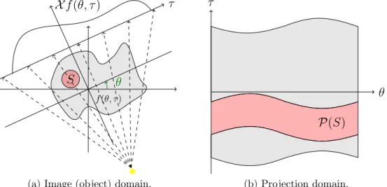
y(θ, τ ) = X f (θ, τ ), θ ∈ [0, 2π), τ ∈ R. (2.2) Notice that T = {(θ, τ ) : θ ∈ [0, 2π), τ ∈ R} is the tangent space of the circle. Also, we will address the domain of (2.2) as the projection domain and the domain of the density or attenuation function as the image domain.
In the ROI tomography problem, projections are collected only for those rays meeting a region of interest inside the field of view. The goal is to recover the density function inside the ROI only, while the rest of the function is essentially ignored, even if the contribution from the object outside the ROI is included into the measured data, because of the overlapping principle of the CT measurements. By denoting with S ⊂ R2 the ROI, the set of ROI-truncated projections is
identi-fied to be the set
X f (θ, τ )
θ
τ
S
f (θ, τ )
(a) Image (object) domain.
P(S)
θ τ
(b) Projection domain.
Figure 2.1: Illustration of the ROI S in the image domain, on the left (a), and the corresponding ROI-truncated projections P(S), on the right (b).
Thus, the ROI reconstruction problem can be formulated as the problem of recon-structing the density function f restricted to the ROI S from the truncated X-ray projections. The geometrical set-up is illustrated in Figure 3.3. Mathematically, this reads as:
y0(θ, τ ) = M (θ, τ ) X f (θ, τ ) with M (θ, τ ) = 1P(S)(θ, τ ) (2.3)
where M is the mask function on T and 1A is the characteristic function of the
set A, defined by
1A(x) =
{
1 if x ∈ A
0 if x ̸∈ A. (2.4)
We will refer to y0(θ, τ ) as the truncated sinogram. In the following, we will assume
that the ROI S is a disk in R2, since it is the more natural choice, due to the circular trajectory of the X-ray source. If pROI ∈ R2 denoted the center of the ROI and
rROI ∈ R its radius, it is clear that
P(S) = {(θ, τ ) ∈ T : |τ − pROI· ωθ| < rROI}.
More general convex ROIs can be taken into account by finding the minimal en-closing disk for such a ROI and reconstructing the image for this disk.
A natural approach for obtaining a stable reconstruction of f from equation (2.3) is by computing the least squares solution ¯f :
¯
f = argmin
f
2.2. FROM CT TO ROI CT: CONTINUOUS SETUP 19 The least squares approach is a state of the art method to solve linear inverse problems of the form (2.2), which can often be motivated for statistical reasons (see Chapter 5 for more details). It can be understood as a data mismatch term since, in general, it accounts for the discrepancy between the actual measurements and the ideal measurements.
However, it is known that the solution of the ROI problem, in general, is not guaranteed to be unique [127] and also the minimizer of problem (2.5) is not unique, since the set of solutions is the affine subspace
V = {f ∈ L2(R2) : y = X f and M y = y0},
given that the kernel of M X is not trivial, i.e., ker(M X ) ̸= {0}, due to the truncation mask operator M . Moreover, even when the uniqueness is ensured, we already remarked that the inversion of the X-ray transform is an ill-posed problem, with the ill-posedness becoming more severe when the projections are truncated, as in the case of the ROI CT problem.
A classical approach to achieve uniqueness is to use the Tikhonov regulariza-tion method [151]. The basic idea of the Tikhonov method is to search for the minimum-norm solution, having incorporate a certain a priori assumptions about the smoothness of the solution by adding an additional norm condition. In details, one seek for the solution of the following minimization problem:
argmin f { ∥Kf − g∥2 2+ µ ∥f ∥ 2 2 } , (2.6)
where K : H1 → H2 is a linear continuous operator between the Hilbert spaces H1
and H2, g ∈ H2 is the measured data and µ ∈ R+, which is usually referred to as
penalty or regularization parameter, controls the weight given to minimization of the additional norm term. Clearly, K = M X and g = y0 according to the notation
introduced in this Chapter. It can be shown that for each µ ∈ R+ the minimum problem 2.6 is equivalent to the Euler equation
(K∗
K + µI)f = K∗g
where K∗ denotes the adjoint operator and I is the identity operator. The impor-tance of the Tikhonov method relies in the following fundamental result.
Theorem 2.3 ([9, 50]). The one-parameter family of operator {Rµ}µ∈R+ defined
by
{Rµ}µ∈R+ =(K∗K + µI
)−1 K∗
is a linear and regular regularization algorithm, in the sense specified by Definition 2.4.