Balanced and imbalanced triads effect on network data

(1)

Università degli Studi di Padova

Dipartimento di Scienze Statistiche

Corso di Laurea Magistrale in

Scienze Statistiche

Balanced and Imbalanced triads effects

on the network structure

Relatore: Prof. Alessandra R. Brazzale Dipartimento di Scienze Statistiche

Correlatore: Prof. Ernst C. Wit Unit of Statistics and Probability University of Groningen

Laureando: Francesco Contin Matricola N. 1034523

(2)

1 Introduction

A social network is a structure in which social agents, such as individuals or organisations, interact with each other. This interaction can be the creation, maintenance or withdrawal of ties. The actors must belong to a meaningfully delineated social group. This delimitation will imply that actors are only studied in this limited pool which on one hand will bound the generality of the study but, on the other hand, yields consistency to the data. The structure can be decomposed into a set of dyadic links between the generic units observed.

The aim of the analysis of a social network is to understand the dynamics that led the network to develop as a whole; the changes in its structure can be due to the characteristics of the network itself and to the actors characteristics. Traditionally, social network analysis had a focus on the rich description of network data, but the recent development of methods of inference for network data has the potential for a wider use [1].

The fields in which the network analysis can be applied are nowadays surprisingly wide, they can be, e.g.:

• Communication studies, which are related to fields such as sociology, psychology, anthropology, political science and economics, as the infor-mation transfer can be studied as a network.

• Diffusion of innovation and ideas, in which the point of interest could be to explain why someone becomes an "early adopter" and someone does not.

• Economic sociology, which considers behavioural interactions of indi-viduals and groups through social capitals and social markets.

• Biological network analysis, which is closely related to the social net-work analysis, but often focusing on local patterns in the netnet-work.

• Social media, since computer networks combined with social networking software produce a new medium for social interaction. This can also include the transfer of informations, goods or services in the real world.

(5)

This list includes only few of the most important fields in which the study of social networks can be applied. Hence, individuals observed can belong to many different environments as, e.g., they can be the pupils of a school whose friendship relations are studied; they can be firms, for which the commer-cial relationships are of interest, or authors of papers for whom the citation frequency is studied.

In this study it is assumed that the ties are directed from an actor to another, and not that the relationship is both ways. Considering the pupils example, it means that if one pupil names another as his/her friend, this does not mean that the second pupil will also name the first as his/her friend; this second actor, in fact, could even dislike the first.

This structure, form a mathematical point of view, is a directed graph, or digraph, where the actors are represented by nodes and the ties between the nodes indicate the presence or absence of a social linkage. The nature of the relationship between the agents leads to structural changes along time which, in turn, affect the actors; this can be interpreted as a mutually de-pendent feedback process. Among the various aspects that can lead a social network to change, we can consider the individual’s characteristics, the net-work characteristics, the pairs of actors’ characteristics and a residual random influence.

The individual’s characteristics can lead the network to change because similar actors are more likely to be interested in each other’s friendship than two actors that have less in common; this effect is usually called "selection". The network characteristics can have an effect as well, e.g. friends of friends becomes friends [2]; this means that the network itself can lead the actors to create or withdraw ties: this effect is usually called "influence". Hence, in this perspective, it is possible to state that the actors will be either conscious or unconscious in the creation or withdrawal of a tie; if the actor’s characteristics lead to the action that modifies the network, this choice will be conscious; on the contrary, if the network’s characteristics will lead it, the choice will be unconscious for the actor. Moreover, not only individual’s characteristics, but also the pairs of actors’ characteristics can be informative about the creation or withdrawal of a tie. The random influences can be seen as aspects that

(6)

cannot be observed about the actors or random events that lead two actors to create or withdraw a tie.

The relationship between selection and influence is one of the most in-teresting aspects in the study of the evolution of a social network, and will be exhaustively covered in the next sections. «In order to distinguish be-tween this two effects, longitudinal data needs to be collected, which at least conceptually opens up the opportunity to study both the processes in par-allel.»(Veenstra et all. 2013,[2]). Longitudinal data consists in repeated observations of the network at different time points, including the collection of the behavioural covariates of the actors. This means that, in order to be able to study the network in this manner, at least two observations of the whole network will be needed. The covariates could be, e.g., the age of the pupils or the family environment in which they live, the smoking attitude for older individuals, or the number of competitors for a firm.

This work focuses on the triads, i.e. the interaction within groups of three individuals. The following steps will be the introduction of the ques-tion of interest on which this work is oriented and the analysis without the use of network-specific models. Afterward the attention will be focused on the evolution of the network and on a network-specific model. At last, the network-specific model introduced will be employed to propose an answer to the question of interest.

(7)

2 Cognitive Dissonance and Balance Theory

The starting point is Fritz Heider’s balance theory on cognitive dissonance. This study will focus on two individuals which are socially related, i.e. like or dislike the each other, and in in this condition form a positive or negative attitude towards a third individual.

The balance theory distinguishes between balanced triads and imbalanced triads [3]. A triad is said to be balanced when two individuals like each other and agree in their attitude towards the third individual, or when they dislike the each other and disagree in their attitude towards the third individual. Instead a triad is said to be imbalanced when they like the each other but they disagree in attitude, or when they dislike the each other and agree in attitude. «According to Heider, humans prefer the cognitive balance. They experience psychological distress when they are in an imbalanced situation and try to create a balanced one by either changing their attitude to the object, or their relationship to the other individual. »(Steglich and Niezink,[3])

(a) Balanced triad named Happy1,

in which two individuals share the same positive attitude they have with a third individual

(b) Balanced triad named Happy2, in

which two individuals in a positive relation share a negative attitude to-wards the third individual

(8)

Figure 2: Balanced triad named Happy3, in which two individuals in a

neg-ative relation disagree in opinion towards a third individual

In this study three kinds of balanced triads have been identified, and named Happy1, Happy2 and Happy3. In Figure 1a it is possible to observe

the first kind of balanced condition, Happy1, looks like in a directed network

representation where the arrows represent the relations and the nodes rep-resent the actors. In this triad the individual marked as "1" is said to be affected: he is the one enjoying the status of balance, as the arrows show in the figure. In Figure 1b it is possible to see the second kind of balanced conditions, in which individual "1" has a positive relation with individual "2" and they share the same, negative, opinion toward individual "3"; in this triad, again, individual "1" is affected.

Figure 2 shows the last possible kind of Heider’s balanced conditions in triads, i.e. the condition in which the individual "1" is affected by the disagreement with individual "2" about the attitude towards individual "3", where with the individual "2" there is a negative attitude.

As for the balanced triads, the imbalanced ones have been divided into three different kinds: Dissonant1, Dissonant2 and Dissonant3. In Figure

3 it is possible to observe the first example of imbalanced conditions: the "affected" individual, marked as "1", is suffering the fact that he/she is not sharing the same attitude towards individual "3", with individual "2" which is considered as a friend.

(9)

Figure 3: Imbalanced triad named Dissonant1, in which the affected

individ-ual disagrees in opinion with an individindivid-ual towards whom there is a positive attitude

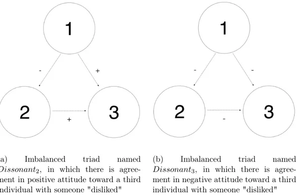
(a) Imbalanced triad named

Dissonant2, in which there is

agree-ment in positive attitude toward a third individual with someone "disliked"

(b) Imbalanced triad named

Dissonant3, in which there is

agree-ment in negative attitude toward a third individual with someone "disliked"

Figure 4: Imbalanced triads in which the affected individual agrees in opinion with an individual towards whom there is a negative attitude

(10)

The other two kinds of imbalanced conditions are shown in Figure 4, and they share the commonality that both are based on an agreement attitude with a "disliked" individual. For consistency reasons, here too the affected in-dividual is "1"; thESE two kinds of imbalanced triads were kept distinguished because, even though they are both based on agreement with someone "dis-liked", the Dissonant2 condition could be considered better than the one in

Dissonant3. This is due to the fact that in the latter all the relations are

negative, whereas in the other, two of the arrows are positive. Since the aim is to understand if these different conditions affect the psychological distress, it is reasonable to think that different amounts of positive relations, although in an imbalanced condition, can differently affect the individuals.

Starting from Heider’s assumption, the aim of this study is to verify, on network data, the effect of the increase or decrease of the quantity of such triads on the individuals’ stress level. The statistical tools used in the first analysis will not be network-specific, but simple as the linear regression model, with mixed effects in order to take into account all the individual’s differences, and generalised additive models.

2.1 The Data

The data hereby introduced will be used along all the study: first with sim-ple models in order to understand what to expect from the balanced and imbalanced triads, later for describing the network as a stochastic process and finally to thoroughly study the network behaviour.

The data is a panel in three waves, collected in a secondary school in Northern Netherlands during the school year 2013/2014. All the 125 pupils belong to the third year, therefore they are between 13 and 16 years old, with an average of 14.3; 64 of them are male and 61 female. The questionnaire’s administration was repeated 3 times (November 2013, February 2014 and May 2014). In each questionnaire, in addition to the network status, it was collected information about the stress level of the pupils, their family status, their hobbies and about their feelings in the past two weeks. Of the 125 pupils participating to the study, 106 were present in all three questionnaires,

(11)

and of these 106 only 86 answered to both the network and stress level questions; when, on the stress level measurement section, the missing data were negligible they were replaced with the mean of the non missing answers. The networks collected in each questionnaire are formally two, one with the friendship relations and one with the dislike relations; solely for the purpose of this section the two networks were overlapped in order to work with one simple structure summarising all the types of relations. Each pupil was asked to nominate in-between 1 and 20 other pupils as friends and the same was asked for the ones he/she dislikes. The network is structured in such a way to be a directed graph, i.e. the relationships are not both ways; if one pupil names the other as a friend it does not necessarily mean that this second pupil will name the first as a friend.

As previously mentioned, three time points are available, which can be seen as different observations in a panel study. This panel is not balanced due to the missing answers, with the consequence that it is not possible to follow the behaviour of all the participants through time; the incomplete paths will be used as much as possible. If the second time point is missing they are basically useless, but if, e.g., only the first or the last time point are missing the evolution can still be studied.

In this section of the study, the number of each balanced and imbalanced condition is compared to a happiness proxy variable in order to understand the relationship between the two. The happiness proxy variable was mea-sured with Likert-scale questions on the agreement with a sentence, on a scale from 1 to 5; the more points a person has, the happier he/she is. The questions used for this variable are:

• I feel comfortable with my friends

• I feel I am part of this school

• Sometimes I feel I do not belong to this school

• I feel very different from most other students at my school.

(12)

• I am proud to belong to this school

• Other students at my school like me as I am

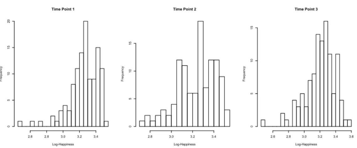
Time Point 1 Log-Happiness F re qu en cy 2.6 2.8 3.0 3.2 3.4 0 5 10 15 20 Time Point 2 Log-Happiness F re qu en cy 2.8 3.0 3.2 3.4 0 5 10 15 Time Point 3 Log-Happiness F re qu en cy 2.6 2.8 3.0 3.2 3.4 3.6 0 5 10 15

Figure 5: Histogram of the logarithm of the Happiness variable in three time points

The sentences with negative meanings are scaled back to allow a compar-ison with the positive ones, by subtracting to 6 the values of the answers. The Cronbach alpha was used in order to measure the reliability of the data; its value is between 0.77 and 0.78 for all the time points, which indicates a fair internal consistency.

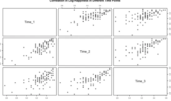
The Happiness variable, since always greater or equal to zero, after a suit-able rescaling, was used in a logarithmic transformation in order to smooth all the peaks and to treat them linearly. Even after the logarithm transfor-mation, which should take care of unusual variance behaviours, the data is asymmetric and it is therefore not possible to state that it has a normal dis-tribution as shown in Figure 5. Furthermore, the nature of the data suggests intra-individual autocorrelation, due to the fact that the happiness level on a time point is likely to depend on the previous happiness status. Moreover, the intra-individual correlation could be also caused by the fact that each person can react differently to changes in their friendship relations. This is shown in Figure 6, where the log-Happiness (from now on Happiness) is plotted against itself at different time points.

(13)

Time_1 2.8 3.0 3.2 3.4 2.6 2.8 3.0 3.2 3.4 2.8 3.0 3.2 3.4 Time_2 2.6 2.8 3.0 3.2 3.4 2.8 3.0 3.2 3.4 3.6 2.8 3.0 3.2 3.4 3.6 Time_3

Correlation in Log-Happiness in Different Time Points

Figure 6: Autocorrelation within the interest variable at different time points: the positive correlation is clear between successive observation and it lightly scatters as time passes between the observations

The correlation between successive time points is high and positive, while, when the time difference is greater, it tends to be less obvious: this could mean that happiness is autocorrelated mostly to its first lag. These aspects will be taken into account in the models.

As previously mentioned, the triads considered are of two kinds, balanced and imbalanced, and both of them are split in three sub-categories; in the balanced condition they are:

• Happy1is a triad in which there is agreement in positive opinion toward

the third person between two individuals with a positive attitude

• Happy2 is a triad in which there is agreement in negative opinion

to-wards the third person between two individuals with a positive attitude

• Happy3is a triad in which there is disagreement in the opinion towards

(14)

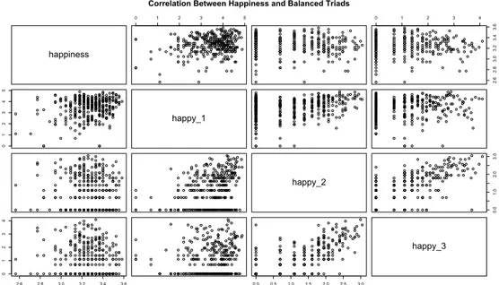
happiness 0 1 2 3 4 5 0 1 2 3 4 2.6 2.8 3.0 3.2 3.4 3.6 0 1 2 3 4 5 happy_1 happy_2 0.0 1.0 2.0 3.0 2.6 2.8 3.0 3.2 3.4 3.6 0 1 2 3 4 0.0 0.5 1.0 1.5 2.0 2.5 3.0 happy_3

Correlation Between Happiness and Balanced Triads

Figure 7: Correlations between all the balanced triads and the Happiness variable

In Figure 7 it is possible to observe that the variable of interest, Happiness, seems to be positively correlated with Happy1 triads; the positive

correla-tion is also present with the other two variables, but in a less obvious way. Furthermore, it is worth mentioning that Happy1 and Happy2 seem to be

positively correlated to each other, as well as Happy2 and Happy3. This

could be related to the fact that all the individuals in Happy1 conditions

belong to a same group of friends, and are therefore more likely to like each other. On the other hand, Happy2 and Happy3 conditions could be

origi-nated from the meeting different groups of friends and, therefore, are more likely to dislike each other.

The imbalanced condition sub-categories are the following:

• Dissonant1 is a triad in which there is disagreement in the opinion

towards a third individual between two individuals with a positive at-titude

• Dissonant2 is a triad in which there is agreement on positive attitude

(15)

at-titude

• Dissonant3 is a triad in which there is agreement on negative

atti-tude toward a third individual between two individuals with a negative attitude happiness 0.0 0.5 1.0 1.5 2.0 2.5 3.0 3.5 0.0 0.5 1.0 1.5 2.0 2.5 2.6 2.8 3.0 3.2 3.4 3.6 0.0 1.0 2.0 3.0 dissonant_1 dissonant_2 0 1 2 3 4 2.6 2.8 3.0 3.2 3.4 3.6 0.0 1.0 2.0 0 1 2 3 4 dissonant_3

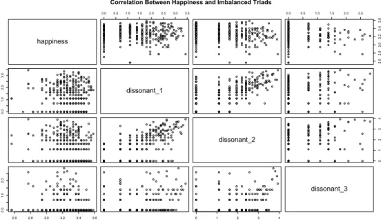
Correlation Between Happiness and Imbalanced Triads

Figure 8: Correlations between all the imbalanced triads and the Happiness variable

Figure 8 shows the correlation between the interest variable, Happiness and the imbalanced triads. The correlation is not obvious as in the previous plot, but, excluding the individuals with little amount of imbalanced condi-tion, there seems to be negative correlation with the interest variable. In this case, the correlation between Dissonant1, Dissonant2 and Dissonant3 can

not be considered as a consequence of inclusion/exclusion from groups, but it probably derives from the "competition" for entering into a group or the process of exiting from one of those.

In order to get an insight about how triads change along time, it is possible to observe their evolution in Table 1 and Table 2, the highest values are on the diagonal, which means that the triads have not changed, or on the bottom line, which means that in the second observation it is not a triad anymore.

(16)

Wave 1 \ Wave 2 Happy1 Happy2 Happy3 Diss1 Diss2 Diss3 N on T riads Happy1 2111 3 2 29 37 0 2796 Happy2 7 60 0 14 7 1 179 Happy3 4 0 86 6 1 0 287 Dissonant1 26 12 2 72 38 1 379 Dissonant2 29 5 5 35 90 0 394 Dissonant3 0 0 7 0 0 4 18 N on T riads 2310 368 576 440 523 114

Table 1: Transition matrix comparing Time Point 1 vs Time Point 2 and all possible triads evolution; Non-Triads means that one or more ties were withdrew and the individuals do not belong to a triad anymore.

Wave 2 \ Wave 3 Happy1 Happy2 Happy3 Diss1 Diss2 Diss3 N on T riads

Happy1 2237 4 3 29 58 0 2157 Happy2 0 132 0 8 12 2 302 Happy3 0 0 197 5 11 3 464 Dissonant1 16 21 9 107 74 0 388 Dissonant2 13 17 18 50 182 1 432 Dissonant3 0 1 0 0 0 16 103 N on T riads 2387 329 423 420 656 100

Table 2: Transition matrix comparing Time Point 2 vs Time Point 3 and all possible triads evolution; Non-Triads means that one or more ties were withdrew and the individuals do not belong to a triad anymore.

2.2 The Models

2.2.1 The mixed effect model

The mixed effect model is an extension of a linear model commonly used in the panel data analysis [5]. This kind of models allow to treat in a different way the effects due the to different individuals considered and the different time points. A general formulation of the model can be written as follows:

Yit= β0+ BXit+ vit

vit = µi+ λt+ uit

uit ∼ IID(0, σ2)

(1)

Examining Equation 1, it is possible to notice that both the response variable and the explanatory ones are both time and individual dependent. The term

(17)

of main interest now is:

vit = µi+ λt+ uit

• µi are the "individual effects" which are the deviation from the mean

due to the effect of each individual. If estimated, they consist in N − 1 parameters, where N is the number of observed individuals in the panel.

• λt are "time effects" which are the deviation from the mean due to the

fact that the panel has different time points. If estimated, they consist in T − 1 parameters, where T is the number of time points.

• uit is the "idiosyncratic component" and it is the generic error term,

which is not due to the time effects or the individual effects.

Now that the model is introduced, before examining in detail the nature of µi and λt, some choices are to be made; they can be summarised in:

• Can the parameters be considered invariant along time?

• Can the parameters be considered invariant among individuals?

They are basically questions about the nature of the terms µi and λt: should

they be considered as random variables or as parameters to be estimated? In order to understand if the parameters in B have to be treated differently for every time point, can be done a statistical test: a comparison between the complete model, the one with all the B for each time point, and the one with B kept constant for all the time points jointly. In this case, the F-test does not reject the null hypothesis, hence the reduced model can be considered as sufficient for the analysis.

On the individual side, considering the data (only 3 observations of 121 individuals), the second option is not acceptable since it would be inappropri-ate to estiminappropri-ate so many parameters in order toproperly treat this component. It is therefore more suitable to treat the individual component as a random effect, having hence:

(18)

The final model will be:

Yit= β0+ BXit+ vit

vit = µi+ uit

where uit∼ IID(0, σ2) ; µi ∼ IID(0, σµ2)

with uit⊥ µi

(2)

The model, estimated with R (package plm), is summarised in the following box. It can be observed that the individual component has a share of about 64% of the total variance and the idiosyncratic component has the remaining 36%. The model, computed on the logarithm transformation of all the vari-ables, is statistically useful since the joint test of nullity for the parameter is widely refused. This model, moreover, explains the 55% of the total variance of the data, thanks to the treatment of the individual component.

Oneway ( i n d i v i d u a l ) e f f e c t Random E f f e c t Model (Swamy−Arora ’ s t r a n s f o r m a t i o n )

C a l l :

plm ( f o r m u l a = form , d a t a = p a n e l , e f f e c t =" i n d i v i d u a l " , model = "random " , random . method = " swar " )

Unbalanced Pan el : n=121 , T=1−3, N=336 E f f e c t s : v a r s t d . dev s h a r e i d i o s y n c r a t i c 0 . 0 0 9 3 2 9 0 . 0 9 6 5 8 8 0 . 3 6 1 i n d i v i d u a l 0 . 0 1 6 5 1 1 0 . 1 2 8 4 9 3 0 . 6 3 9 t h e t a :

Min . 1 s t Qu . Median Mean 3 rd Qu . Max . 0 . 3 9 9 1 0 . 6 0 1 9 0 . 6 0 1 9 0 . 5 9 2 1 0 . 6 0 1 9 0 . 6 0 1 9

(19)

R e s i d u a l s :

Min . 1 s t Qu . Median Mean 3 rd Qu . Max .

−0.45800 −0.05010 0 . 0 1 2 3 0 0 . 0 0 0 8 6 0 . 0 7 0 8 0 0 . 2 1 4 0 0 C o e f f i c i e n t s : E s t i m a t e Std . E r r o r t−v a l u e Pr ( >| t | ) ( I n t e r c e p t ) 3 . 1 4 3 7 3 5 8 0 . 0 3 6 3 6 3 2 8 6 . 4 5 3 7 < 2 . 2 e −16 ∗∗∗ happy_1 0 . 0 5 3 9 7 0 4 0 . 0 1 1 2 2 9 6 4 . 8 0 6 1 2 . 3 5 e −06 ∗∗∗ happy_2 0 . 0 1 5 6 8 7 8 0 . 0 1 3 3 5 5 1 1 . 1 7 4 7 0 . 2 4 0 9 8 happy_3 −0.0078647 0 . 0 1 0 7 6 6 1 −0.7305 0 . 4 6 5 6 0 d i s s o n a n t _ 1 −0.0243914 0 . 0 1 2 2 8 3 1 −1.9858 0 . 0 4 7 8 9 ∗ d i s s o n a n t _ 2 −0.0161602 0 . 0 0 9 0 6 6 4 −1.7824 0 . 0 7 5 6 1 . d i s s o n a n t _ 3 −0.0087444 0 . 0 1 4 5 0 2 8 −0.6029 0 . 5 4 6 9 6 t i m e 2 −0.0066872 0 . 0 1 3 8 9 0 7 −0.4814 0 . 6 3 0 5 4 t i m e 3 −0.0353904 0 . 0 1 4 3 4 7 3 −2.4667 0 . 0 1 4 1 5 ∗ S i g n i f . c o d e s : 0 ’ ∗ ∗ ∗ ’ 0 . 0 0 1 ’ ∗ ∗ ’ 0 . 0 1 ’ ∗ ’ 0 . 0 5 ’ . 0 . 1 ’ ’ 1 T o t a l Sum o f S q u a r e s : 6 . 7 5 7 9 R e s i d u a l Sum o f S q u a r e s : 3 . 0 6 7 2 R−Squared : 0 . 5 5 1 1 4 Adj . R−Squared : 0 . 5 3 6 3 8 F− s t a t i s t i c : 4 9 . 1 8 on 8 and 327 DF, p−v a l u e : < 2 . 2 2 e −16 Model’s Findings

Since the data is an unbalanced panel the use of a particular method (SWAR) is mandatory in order to estimate the variance; this solution is preferable to eliminating some observations to obtain a balanced panel. Considering that the variation range of the response variable is around 1, it is possible to proceed with the analysis of the coefficients estimation. Happy1 has a high

(20)

is statistically different from zero. Happy2 and Happy3, on the other hand,

are not statistically different from zero, which allows to state that their effect is not relevant for the study. Moreover, it is possible to notice that two of the coefficients of the balanced triads are positive and that the last one (Happy3,

which represents disagreement with someone disliked) is not. These kinds of triads are difficult to analyse because, although the disagreement can balance the condition, it is not empirically proven whether it is the disagreement with someone "disliked" or the negative attitude itself that creates the distress condition.

The parameters of the imbalanced condition are all negative, and two out of three are statistically different from zero. Dissonant1, disagreement with

someone liked, can be considered as a stressing condition, since the parame-ter is negative and consequently the presence of this kind of triads negatively affects the response variable. Dissonant2, agreement with someone disliked,

can be interpreted as the previous parameter with the only distinction that its value is smaller. The last imbalanced condition found in the theory is Dissonant3, where all the individuals dislike the each other. This parameter

is highly non significant which allows to state that perhaps, in a condition where between two individuals there is a negative attitude, it does not sig-nificantly affect the overall happiness if the third individual is disliked.

The last parameters concern the time points and were introduced in order to evaluate if they can be considered as homogeneous. The first and the sec-ond time point can be considered homogeneous since the coefficient for the dummy variable is not statistically different from zero. The first time point and the third, however, are not homogeneous; this could be a consequence of the fact that longer time passed between the first and the last administration of the questionnaire. This result does not significantly affect the use of com-mon parameters for all the time points since the "poolability" test carried out in the first part of the analysis allowed such a treatment.

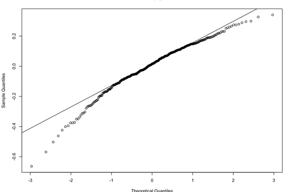
Figure 9 shows how the sample residuals distribute with respect to the theoretical ones; the model does not estimate accurately the extreme values, which are distant from a normal distribution, but it fits accurately the central values. The bias of the model is that all the extreme values are

(21)

underesti--3 -2 -1 0 1 2 3 -0 .4 -0 .3 -0 .2 -0 .1 0.0 0.1 0.2 Normal Q-Q Plot Theoretical Quantiles Sa mp le Q ua nt ile s

Figure 9: Quantile-Quantile plot of the mixed effects model residuals, where the normality is not completely fulfilled since all the extreme values are un-derestimated

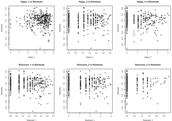
mated as all of them are under the theoretical distribution line. In Figure 10 it is possible to observe how the residuals distribute with respect to every response variable, and it does not appear any systematic behaviour in it.

(22)

0 1 2 3 4 5 -0 .4 -0 .3 -0 .2 -0 .1 0.0 0.1 0.2 Happy_1 vs Residuals Happy_1 R esi du al s 0.0 0.5 1.0 1.5 2.0 2.5 3.0 -0 .4 -0 .3 -0 .2 -0 .1 0.0 0.1 0.2 Happy_2 vs Residuals Happy_2 R esi du al s 0 1 2 3 4 -0 .4 -0 .3 -0 .2 -0 .1 0.0 0.1 0.2 Happy_3 vs Residuals Happy_3 R esi du al s 0.0 0.5 1.0 1.5 2.0 2.5 3.0 3.5 -0 .4 -0 .3 -0 .2 -0 .1 0.0 0.1 0.2 Dissonant_1 vs Residuals Dissonant_1 R esi du al s 0 1 2 3 4 -0 .4 -0 .3 -0 .2 -0 .1 0.0 0.1 0.2 Dissonant_2 vs Residuals Dissonant_2 R esi du al s 0.0 0.5 1.0 1.5 2.0 2.5 -0 .4 -0 .3 -0 .2 -0 .1 0.0 0.1 0.2 Dissonant_3 vs Residuals Dissonant_3 R esi du al s

Figure 10: Residuals versus all the explanatory variables included in the model, exception made for the time dummy variables; does not seem to be systematic

2.2.2 The generalised additive models

The second family of models applied is the generalised additive models (GAM); this kind of models consist of fitting a predictor for each variable and col-lecting in an additive fashion all the outcomes [4]. This way of acting has less model-specific constraints than the linear model and will be able to col-lect more variable-specific behaviours. The model can be formally written as follows:

Happiness = α0+ f1(Happy1) + f2(Happy2) + f3(Happy3)+

+ f4(Dissonant1) + f5(Dissonant2) + f6(Dissonant3)+

+ T ime + ε

(3)

(23)

of functions are piecewise third degree polynomials. One of the tuning pa-rameters for this estimation procedure is the number of polynomials to use or, more precisely, the number of knots in which the basis functions will match to create a unique polynomial function. For the purpose of this study, the cu-bic splines will be fitted to the data through regressions spline. The dummy variables in this kind of models will affect the smooth polynomial fitting the data, as a baseline effect, rising or reducing their height. In this kind of models the number of parameters and, hence, of splines fitted is significantly important and it is not possible to use a tool allowing to differentiate all the individuals. Although this possibility is not available, it is still worth to consider this smooth fitting in order to understand the overall behaviour of the balanced and imbalanced triads with respect to the Happiness dependent variable chosen. The following box shows the summary of the model:

Family : g a u s s i a n Link f u n c t i o n : i d e n t i t y Formula : h a p p i n e s s ~ s ( happy_1 , bs=" c r ")+ s ( happy_2 , bs =" c r ")+ + s ( happy_3 , bs=" c r ")+ s ( d i s s o n a n t _ 1 , bs=" c r ")+ +s ( d i s s o n a n t _ 2 , bs=" c r ")+ s ( d i s s o n a n t _ 3 , bs=" c r ")+ t i m e P a r a m e t r i c c o e f f i c i e n t s : E s t i m a t e Std . E r r o r t v a l u e Pr ( >| t | ) ( I n t e r c e p t ) 3 . 2 8 1 5 2 2 5 0 . 0 1 5 3 7 6 4 2 1 3 . 4 1 2 <2e −16 ∗∗∗ t i m e 2 −0.0004642 0 . 0 2 1 8 4 7 2 −0.021 0 . 9 8 3 t i m e 3 −0.0265384 0 . 0 2 2 2 1 7 7 −1.194 0 . 2 3 3 −−− S i g n i f . c o d e s : 0 ’ ∗ ∗ ∗ ’ 0 . 0 0 1 ’ ∗ ∗ ’ 0 . 0 1 ’ ∗ ’ 0 . 0 5 ’ . ’ 0 . 1 ’ ’ 1

(24)

Approximate s i g n i f i c a n c e o f smooth t e r m s : e d f Ref . d f F p−v a l u e s ( happy_1 ) 1 . 7 4 5 7 2 . 1 8 1 1 4 . 4 3 2 5 . 4 1 e −07 ∗∗∗ s ( happy_2 ) 1 . 0 0 8 7 1 . 0 1 7 0 . 4 8 9 0 . 4 8 7 0 7 s ( happy_3 ) 0 . 9 9 9 8 1 . 0 0 0 0 . 0 8 6 0 . 7 6 8 9 1 s ( d i s s o n a n t _ 1 ) 1 . 3 2 3 0 1 . 5 6 8 0 . 6 7 3 0 . 4 5 9 7 4 s ( d i s s o n a n t _ 2 ) 0 . 9 9 9 8 1 . 0 0 0 6 . 8 8 5 0 . 0 0 9 0 9 ∗∗ s ( d i s s o n a n t _ 3 ) 1 . 0 0 0 0 1 . 0 0 0 1 . 3 4 4 0 . 2 4 7 0 8 −−− S i g n i f . c o d e s : 0 ’ ∗ ∗ ∗ ’ 0 . 0 0 1 ’ ∗ ∗ ’ 0 . 0 1 ’ ∗ ’ 0 . 0 5 ’ . ’ 0 . 1 ’ ’ 1 R−s q . ( a d j ) = 0 . 1 3 9 D e v i a n c e e x p l a i n e d = 16.2% GCV s c o r e = 0 . 0 2 6 2 2 2 S c a l e e s t . = 0 . 0 2 5 4 3 6 n = 336 Model’s Findings

This model has an explanatory capacity of about 16%; the difference with the adjusted R-squared could be interpreted as an high consumption of degrees of freedom due to the number of knots used in the splines fitting (ten each). Nevertheless, using ten degrees of freedom seemed to be the best compromise between smoothness and precise fitting.

In this model, as in the one introduced before, the intercept has an impor-tant role; however the time dummy variables lose their meaning confirming the fact that the three time points can be considered as homogeneous. For what concerns the balanced triads variables, only Happy1 has a statistically

significative effect, and in the imbalanced condition the same is true for Dissonant2.

In order to understand the behaviour of the regression splines used in the model, it is useful to refer to Figure 11; since this kind of models matches different polynomials, a convenient way to interpret it is to observe how the matched polynomial looks like. The outcome of the model will be the sum of these behaviours. It is possible to observe that Happy1 splines have a

(25)

0 1 2 3 4 5 -0 .6 -0 .4 -0 .2 0.0 0.2 0.4 happy_1 s(h ap py_ 1, 1. 75 ) 0.0 0.5 1.0 1.5 2.0 2.5 3.0 -0 .6 -0 .4 -0 .2 0.0 0.2 0.4 happy_2 s(h ap py_ 2, 1. 01 ) 0 1 2 3 4 -0 .6 -0 .4 -0 .2 0.0 0.2 0.4 happy_3 s(h ap py_ 3, 1) 0.0 0.5 1.0 1.5 2.0 2.5 3.0 3.5 -0 .6 -0 .4 -0 .2 0.0 0.2 0.4 dissonant_1 s(d isso na nt _1 ,1 .3 2) 0 1 2 3 4 -0 .6 -0 .4 -0 .2 0.0 0.2 0.4 dissonant_2 s(d isso na nt _2 ,1 ) 0.0 0.5 1.0 1.5 2.0 2.5 -0 .6 -0 .4 -0 .2 0.0 0.2 0.4 dissonant_3 s(d isso na nt _3 ,1 )

Figure 11: Gam behaviour spilt in each component (explanatory variable), the result of the model is the sum of all these behaviours

positive effect on the happiness level. Happy2 and Happy3 do not seem to

have any relevant effect on the dependent variable in this model; this was noticed as well in the summary of the model, in which those splines were not significantly different from zero. The splines referring to the imbalanced condition seem all to have a negative effect, but only Dissonant2 is actually

significative.

In the Quantile-Quantile plot of Figure 12 it is possible to observe that the GAM model as well underestimates the extreme values of the dependent variable, but it seems to be more consistent with the high values compared to the mixed effect model; in any case, the distribution is not totally satisfying the normality assumption.

(26)

-3 -2 -1 0 1 2 3 -0 .6 -0 .4 -0 .2 0.0 0.2 Normal Q-Q Plot Theoretical Quantiles Sa mp le Q ua nt ile s

Figure 12: Quantile-Quanitle plot of the GAM model’s residuals, there is an underestimation of the extreme values

2.3 Conclusions

The initial question was whether balanced and imbalanced conditions can increase the happiness level in the individuals. What the models have shown is that, on average, the presence of balanced triads can lead to an increase of happiness. Both models agree on the fact that only Happy1 condition has

a significant effect on the happiness level. Consequently it seems that only the agreement in opinion between two individuals that like each other has an overall effect, whereas the other balanced conditions, e.g. the disagreement with someone which is disliked, do not affect the happiness level.

The imbalanced condition, as expected, has a negative effect on the hap-piness of the average individual. Dissonant2 was selected by both models to

have negative and significant effect on the happiness level; Dissonant1 was

(27)

effect in both the models; it therefore seems adequate to consider it as an interesting variable. The Dissonant3 was not significative in any models; it

will therefore not be considered in the future. The variables that resulted significant will be introduced in the network study and the results will be compared with the ones of this first step.

2.3.1 Discussion

Only three time points were available for this analysis. Although they seemed to be homogeneous, this does not necessarily mean that different time points would lead to the same results. It could be possible that, if more time points are available, two distant observations of the network, as well as the parameters of the independent variables, are not statistically homogeneous.

However, having more observations of the whole network could lead to a more precise estimation, and also, at some point, to estimate the µi effects

in the mixed effects model. This estimation would lead to a model that can find the overall behaviour with regard to the independent variables and at the same time take into account the differences of the actors involved in the study.

The lack of more observations and the use of few explanatory variables of interest led the residuals not to have a normal distribution, as assumed from the models. In the linear model quantile-quantile plot it is possible to observe that some residuals in the margins of the plot are far from the theoretical distribution; this could be due to the heteroscedasticity of the residuals, introducing in the model an underestimation of the variance of the parameters. On the other hand, the GAM model was able to collect in a more precise way the variability of the data with lower values; however, it has an underestimation problem for higher values. The logarithmic transformation seems to have a good effect on the heteroscedasticity, but at some time it does not seem to be sufficient.

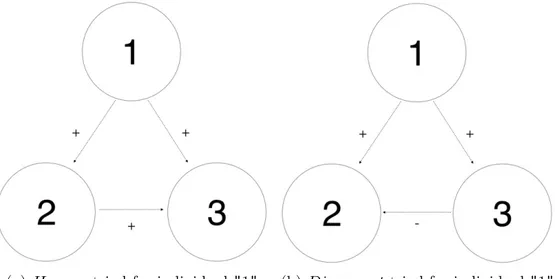
Moreover, as shown in Figure 13, also the structure of the triads deserves some remarks. In both triads individual "1" is affected, with the only dif-ference of the relation between individual "2" and "3". Figure 13a shows

(28)

(a) Happy1 triad for individual "1" (b) Dissonant triad for individual "1"

Figure 13: Two triads with "affected" individual element "1" and composed by the same individuals, triad 13a is counted as balanced and triad 13b is counted as imbalanced

the "Happy1" triad, composed by the elements "1", "2" and "3", in which

individual "1" is affected. Figure 13b shows the "Dissonant2" triad, as well

composed by the elements "1", "2" and "3", in which individual "1" is af-fected. This implies that the same triad is both balanced and imbalanced. It was not possible to understand if, and to what extent, this could be mis-leading. One possible solution is to change the definition of the triads and consider the both-way friendship; however, using this solution the number of triads in the network would decreased significantly, therefore losing impor-tant information.

(29)

3 Networks as a Stochastic Process

A the network is defined as a set of links between some actors, i.e. a set of arrows (representing the links) connecting some nodes (representing the ac-tors). Since these sets can vary in their composition, they can be understood as a dynamic process, whose consequent evolution can be understood as a stochastic process, although for this second step some more assumptions are required. Ties can be established, gain strength or be dissolved, and this can happen in all kinds of relation such as friendship, sales agreement or cell in-teraction [6]. Every change in the network will be driven by multiple factors, such as the characteristics of the considered nodes or the characteristics of the network itself. This second aspect will be analysed in the next sections since it is one of the core aspects used in modelling.

The peculiar and statistically relevant aspect of the networks is that they are not composed of independent observations, indeed all the changes in the network will cause consequent effects: creation of new ties or withdraw of the existing. It is possible to state that every change in the network depends, given all the other observed variables as fixed, on its first shape, which leads to the definition of a Markov chain.

A Markov chain is a stochastic process in which the probability distribu-tion of future states, in this case the shape of the network, depends only from the last status. This can be easily observed in a particular kind of networks in which only one change at the time is allowed: the new state that will be reached depends solely on the actual state which, in turn, depends only on the preceding state. This assumption cannot be said as realistic but, with the available data and the complexity of the real process, it is the better available [7]. In this first introduction of the network as a Markov chain stochastic process, a simple network structure will be used: the one with dichotomous variables indicating the presence or absence of a like or friendship relation. This will later be extended to the case in which other kinds of relation are allowed, as in the multilevel network, where both likes and dislikes appear.

(30)

3.1 Definition of the process

At this point, a rigorous notation is needed in order to exactly define the process and try to explain its evolution. The network can be represented by the set of every possible tie; hence, an adjacency matrix, X(t) is defined, so that it will depend on the time t in which the network is observed, with generic element xi,j(t). This last element will point out whether there is a

relation between the two actors or not.

Xi,j =

(

1 if there is a like relation between actor i and actor j 0 otherwise

Xi,j(t) is a time dependent random variable, and it may also depend on other

explanatory variables which can be either time invariant or change with the time [7].

It is now worth to further explain the distinction between the actual process that allows the network to evolve and its possible observations. The evolution of the network, as stated before, can be considered as a dynamic process that, although split in mini-steps allowing only one change at the time, is not possible to be observed directly in most of the applications. In social studies, e.g., it is not possible to administrate a questionnaire every day in order to evaluate every single change and, perhaps, even so it would not be possible to gather all the changes. The questionnaire administrations along time are few (in order to be able to work with the data at least 2) and the changes collected between the two time points are important for the study. Hopefully they are neither radically different nor considerably similar. Once two observations of the whole network are available, it is possible to compare them and suppose that there are K changes between the two time points. What the observer can state is that there were at least K + 2S with S ∈ [0, 1, 2, . . . ) changes. Suppose now that the observer wants to estimate, through a simulation, the evolution of the network between the two time points: the most straightforward way to do it is to consider a continuous time Markov chain.

(31)

process is that the future only depends on the present status of the network, which can be extended to the continuous time as follows: {X(t) | t ∈ T } is a stochastic process with a finite outcome space X ; {X(t) | t > ta} depends

only on the present X(ta) and with ta< tb , x ∈X it is possible to state that:

P (Y (tb) = x | X(t) = x(t) ∀ t ≤ ta) = P (Y (tb) = x | X(ta) = x(ta)) (4)

The process, in this case, is only a function of the elapsed time between ta

and tb. If {X(t) | t ∈ T } is a continuos time Markov chain with stationary

transition distribution, it is possible to find the intensity matrix of the in-finitesimal generator as follows:

q(x, y) = lim dt→0 P (X(t + dt) = y | X(t) = x) dt for x 6= y q(x, x) = lim dt→0 1 − P (X(t + dt) = x | X(t) = x) dt (5)

This matrix expresses the probability of each change in the network as the elapsed time tends to zero. y is an adjacency matrix with only one differing element form x, an adjacency matrix as well [8].

3.1.1 Who makes the move and when: the rate function

Until now, no assumptions on the decision process for creating or withdrawing a tie were made; it will be now explained how the actors change their ties. It is natural to assume that the actor has the complete control of the ties: he/she can decide whether to create or withdraw a tie no matter if the receiving actor agrees. The instant of time in which the change happens is defined by a rate function which indicates how frequently the actors make a move:

λi(x) = lim dt→0

1

dtP {Xit(t + dt) 6= Xit(t) f.s. j ∈ {1, . . . , g}|X(t) = x} (6) where g is the number of actors in the network [8].

(32)

constant for all the actors, said ρ: λi(x) = ρ ∀ i. It is also assumed that

there is independence between the actors in the elapsed time ∆t in which they make the ministep. The waiting time between successive ministeps for each actor will have an exponential distribution, hence the expected number of changes will be gρ(tb − ta): it depends from the number of actors in the

whole network (g), the changing rate (ρ) and the interval of time considered (tb − ta).

The easiest condition is a good starting point; however, when some co-variates on the behaviour of the actors are available, it is natural to assume that those have different behaviours in terms of waiting time before the next ministep. It is useful to introduce the covariates taking into account the fact that the final rate parameter must be positive; one efficient proposal is:

ρi(α, x) = ρmexp X h αhvhi ! , (7)

where Vh are all the covariates available. This rate function can be

fur-ther extended in order to include furfur-ther aspects of the network such as the number of outgoing ties an actor has, or the number of incoming ties, etc.; all these network dependent variables will be used as the other covariates, keeping into account that this kind of data can vary from one ministep to the other. Now that the exponential distribution for each actor has been defined, it is straightforward to define the overall process distribution. Con-sidering λ+(x) = Pg_i=1λi, it is possible to use an exponential distribution

with parameter λ+(x) for the random variable defining the time interval ∆t

between the ministeps (the definition of λ+(x) is derived from a property of

the exponential distribution, explained more extensively in section 3.2.1). Once the process timing for the next move has been defined, the actor making the move must be decided. In the simulation process it will be chosen randomly with probability λi(x)

(33)

3.1.2 Which change to make

After deciding how much time has passed from the last change and which actor will create or withdraw a tie, the next step is to make the actual change. Suppose that the chosen actor at time t + ∆t is i; there are g − 1 possible other actors with whom the relation can change. More precisely, for the simple network so far considered, the change between the chosen actor i and another actor j will be: Xi,j(t + ∆t) = 1 − Xi,j(t). The probability

distribution for the choice of the second actor involved in the change will depend on the characteristics of the two actors and on the network status; the latter involves the network as it is at time t and how it could be at time t + ∆t. The tool used in this step is called "objective function" which will be properly introduced later (section 4.5); at this moment, it is enough to know that it is a function in which the aforementioned data is included and weighted with the estimated parameters. The function defining the change of the relation between actor i and actor j can be written as follows:

fi(X(i j)) (8)

In order to compute the probability, this function will be divided by the sum of all the other possible outcomes as normalising constant; moreover, an exponential transformation will be used in order to maintain all the values positive. The result is as follows:

Pij =

exp {fi(X(i j))}

Pg

h=1,h6=iexp {fh(X(i j))}

(9)

Pij gives the mass probability function for all possible js, and from this mass

function the actual j which will be included in the move will be sampled. The rate parameter introduced in the previous section is usually constant between two network observations, as well as in all the ministeps incurring between the two. The objective function strongly depends on the network structure and, although the parameters in it are constant, it changes its outcome in each ministep.

(34)

3.1.3 Example

The aim of this section is to apply the discussed evolution procedure to an empirical example. For this purpose a small set of the data introduced in section 2.1 is used. The whole dataset, as mentioned, collects the data from 125 pupils. Here only a class (the second) composed by 25 of them is considered. All the outgoing or incoming ties outside of the class were ignored. The next steps will be: the representation of the data in a graph structure, the adjacency matrix and some steps of the stochastic process.

Firends class 2 wave 1 1 2 3 4 5 6 7 8 9 10 11 12 13 14 15 16 17 18 19 20 21 22 23 24 25

Figure 14: Network representation in graph form of pupils relations within one class

In Figure 14 it is possible to observe the representation of the simple net-work, with only one possible relation (friendship), where the arrows represent the relations and the nodes represent the individuals.

(35)

[,1] [,2] [,3] [,4] [,5] [,6] [,7] [,8] [,9] [,10] [,11] [,12] [,13] [,14] [,15] [,16] [,17] [,18] [,19] [,20] [,21] [,22] [,23] [,24] [,25] [1,] 0 1 0 1 1 0 0 0 0 1 0 0 1 0 0 0 0 0 1 0 0 0 0 1 0 [2,] 1 0 0 0 1 0 0 0 1 0 1 0 1 0 0 0 0 0 1 0 0 0 0 1 0 [3,] 1 1 0 0 1 0 0 1 0 0 1 0 1 1 0 0 0 1 0 1 0 0 1 1 1 [4,] 0 0 0 0 0 0 0 0 0 0 0 0 0 0 0 0 0 0 0 0 0 0 0 0 0 [5,] 1 1 0 0 0 0 0 0 1 1 1 0 1 0 0 0 0 1 1 0 0 0 0 1 0 [6,] 0 0 0 1 0 0 0 0 0 0 0 0 0 1 1 1 1 0 0 0 0 1 0 0 0 [7,] 1 0 0 1 0 0 0 0 0 0 0 1 0 0 0 1 0 1 1 0 1 0 1 1 0 [8,] 0 0 0 0 0 0 0 0 0 0 0 0 0 0 0 0 0 0 0 1 0 0 1 0 1 [9,] 0 0 0 0 0 0 0 0 0 0 0 0 0 0 0 0 0 0 0 0 0 0 0 0 0 [10,] 0 0 0 0 0 0 0 0 0 0 0 0 0 0 0 0 0 0 0 0 0 0 0 0 0 [11,] 1 1 1 0 1 0 0 0 0 0 0 0 1 0 0 0 0 1 0 0 0 0 0 1 0 [12,] 0 0 0 1 1 0 1 0 1 0 0 0 1 1 0 1 0 0 1 0 1 0 1 0 0 [13,] 1 1 1 0 1 0 0 0 1 1 1 0 0 0 0 0 0 0 0 0 0 0 0 1 0 [14,] 0 0 0 1 0 1 0 0 1 0 0 1 0 0 1 1 1 1 0 0 0 1 1 0 0 [15,] 0 0 0 1 0 1 0 0 0 0 0 0 0 1 0 1 1 0 0 0 0 1 0 0 0 [16,] 0 0 0 1 0 1 0 0 0 0 0 1 0 1 1 0 1 1 0 0 1 1 1 0 0 [17,] 0 0 0 1 0 1 0 0 0 0 0 0 0 1 1 1 0 0 0 0 0 1 0 0 0 [18,] 0 0 0 0 0 0 0 0 0 0 0 0 0 1 0 1 0 0 1 0 0 0 0 1 1 [19,] 0 1 0 1 0 0 0 0 1 1 0 1 0 0 0 1 0 1 0 0 0 1 0 1 0 [20,] 0 0 1 0 0 0 0 1 0 0 0 0 0 1 0 1 0 1 0 0 0 0 1 0 1 [21,] 0 0 0 0 0 0 1 0 0 0 0 1 0 1 0 1 0 0 1 0 0 0 0 0 0 [22,] 0 0 0 1 0 1 0 0 0 1 0 1 0 1 1 1 1 1 1 0 0 0 0 0 0 [23,] 0 0 0 0 0 0 0 1 0 0 0 0 0 1 0 1 0 1 0 1 0 0 0 0 1 [24,] 1 1 0 1 1 0 0 0 1 1 1 0 1 1 0 0 0 1 1 0 0 0 0 0 0 [25,] 0 0 1 0 0 0 0 1 0 0 0 0 0 0 0 0 0 1 0 1 0 0 1 0 0

Figure 15: Network adjacency matrix

The matrix in Figure 15 is the adjacency matrix which creates the network and the process; the "1" between two individuals stands for the presence of a relation, whereas the "0" stands for absence of relation.

The next step is to simulate its evolution given some network-based in-formation and some covariates. In order to have a reliable simulation of the process, the network was studied with the RSiena package in R, and the pa-rameters obtained will be used for the simulation [9] [10]; the procedure for the estimation will be explained in detail in sections 4.8 - 4.10. The software estimated a rate parameter (ρ) of 4.18; consequently each individual, on av-erage, has about 4 chances to change in the elapsed time between the two observations. Hence, the time before the next move in the network follows an exponential distribution with parameter ρ, which is constant for all the individuals. Once the focal actor, the actor creating or withdrawing a tie, is chosen, the function generating the discrete probability distribution for the move can be summarised as follows:

fi = exp {β1si1(x) + β2si2(x) + β3si3(x) + β4si4(x) + β5si5(x, w)} . (10)

(36)

• si1 is the out-degree density, which stands for the number of outgoing

ties each individual has (Pg

h=1xih)

• si2 is the reciprocity, which stands for the number of reciprocated

rela-tions (Pg

h=1xihxhi)

• si3 is the in-degree popularity, which stands for the number of ingoing

ties to the other individual (Pg

h=1xjh)

• si4 is the out-degree popularity, which stands for the number of

outgo-ing ties from the other individual (Pg

h=1xhj)

• si5is the interaction between same gender and friendship, (Pg_h=1xihwih

where wih = 1 if i and h are both of the same gender)

obtaining the final formula:

fi = exp ( β1 g X h=1 Xih+ β2 g X h=1 XihXhi+ β3 g X h=1 Xjh+ β4 g X h=1 Xhj + β5 g X h=1 Xihwih ) and Pij = exp {β1si1+ β2si2+ β3si3+ β4si4+ β5si5} Pg z=1,z6=iexp {β1si1+ β2si2+ β3si3+ β4si4+ β5si5} (11)

As for the rate parameter, also β1, β2, β3, β4 and β5 were estimated; they will

have the following values:

Parameters β1 β2 β3 β4 β5

Values -1.29 1.67 0.07 0.03 0.09

Table 3: Parameters estimation for the example network

Suppose now the the process is at time 0; the next event will happen at time ∆t with ∆t ∼ EXP (ρ). For the simulation purpose, a value from this distribution will be sampled. Once the time for the next event is defined, an actor will be sampled; since all the actors have the same rate function, the focal one will be extracted from a discrete uniform distribution where all

(37)

the actors have the same probability. After the focal actor has been chosen, the mass probability function for the tie to change is obtained with Formula 11. Finally, the second actor in the evolution process will be sampled from this mass probability function. The process is now showed with a numerical example.

Example of one mini-step

A random time from an exponential distribution with ρ = 4.18 is sampled: 0.318. This is the time instant in which the first change happens, and the sampled actor is: 14. The values obtained from Formula 10 are:

[ 1 ] 8 . 7 0 8 . 7 0 6 . 1 1 1 4 . 0 6 8 . 2 0 7 . 8 2 5 . 8 3 8 . 7 2 [ 9 ] 1 0 . 7 1 1 0 . 0 0 7 . 5 9 7 . 4 3 8 . 4 4 0 . 0 0 7 . 8 2 1 1 . 1 8 [ 1 7 ] 7 . 8 2 1 2 . 9 7 9 . 3 9 7 . 7 5 7 . 0 3 7 . 4 3 1 0 . 4 7 8 . 8 5 [ 2 5 ] 1 0 . 0 8

Plugging in the results in Formula 11, the mass probability function ob-tained is:

[ 1 ] 0 . 0 3 9 0 . 0 3 9 0 . 0 2 7 0 . 0 6 3 0 . 0 3 7 0 . 0 3 5 0 . 0 2 6 0 . 0 3 9 [ 9 ] 0 . 0 4 8 0 . 0 4 5 0 . 0 3 4 0 . 0 3 3 0 . 0 3 8 0 . 0 0 0 0 . 0 3 5 0 . 0 5 0 [ 1 7 ] 0 . 0 3 5 0 . 0 5 8 0 . 0 4 2 0 . 0 3 5 0 . 0 3 1 0 . 0 3 3 0 . 0 4 7 0 . 0 3 9 [ 2 5 ] 0 . 0 4 5

Finally, the tie, or the missing tie, to be changed can be extracted from this discrete distribution. In this case, proceeding with the simulation, the second actor will be: 25. The change in a mathematical form is X14,25(0.318) =

1 − X14,25(0).

The described procedure shows how the ministeps are the core of the network evolution. In order to be able to properly notice the differences between the networks, two simulations were conducted (Figure 17 - 18): the first including 10 ministeps and the second including 50 ministeps, both starting from the network in Figure 14.

(38)

1 2 3 4 5 6 7 8 9 10 11 12 13 15 16 17 18 19 20 21 22 23 24 25 Probability Distribution the Friendship Network

Actors Pro ba bi lit y 0.00 0.02 0.04 0.06 0.08

Figure 16: Mass probability function for the choice of the second individual in the network given the focal actor 14

This simulation does not take into consideration of all the aspects it should in order to show a complete representation of the network evolution. It

vrienden wave 2 1 2 3 4 5 6 7 8 9 10 11 12 13 14 15 16 17 18 19 20 21 22 23 24 25

(39)

vrienden wave 2 1 2 3 4 5 6 7 8 9 10 11 12 13 14 15 16 17 18 19 20 21 22 23 24 25

Figure 18: Graph representation of the network after 50 simulated ministeps

can be noticed that the network evolves in a compact way (no individuals are left apart), which in the social sciences field in not common. The behaviour of the individuals and further aspects of the network should be taken into account in order to exhaustively simulate the evolution. It is not worth, hence, any inference on the parameters computed so far.

3.2 Multilevel Process

Suppose now to have a more complex process to study, in which different kinds of relations are admitted within the same set of individuals. Like and dislike relations between pupils in a school compose the network hereby considered, but multilevel networks can be extended to plenty of fields. In order to make this process feasible, it is assumed that an individual can have only one kind of relation toward another individual in the same instant, e.g. either he/she likes or dislikes the other individual. This attitude can change along time, but in a single time observation only one of the two options is viable.

(40)

The data comes from two distinct networks including the same individ-uals; both levels are represented with the presence or absence of a specified relation. This leads to a multilevel network in which either there is a relation between the nodes or there is not and, when a relation is present, it can be of two different kinds: like or dislike.

3.2.1 Process description

In this section, the two networks will be overlapped and studied based on their characteristics. The difference with the facilitated process is that here the first decision to be made is on which level, between the two available, a change will be made. Once the level is selected, it is possible to refer to the facilitated single-level network process.

In order to chose the level of the network, a rate function which will define the time for the successive move will be used; this same function will also define the mass probability function for the level of the network. The rate function has to be defined in a more exhaustive way: it will be, as in the single-level network, an exponential distribution for both networks involved in the multilevel process. Therefore, there will be two rate parameters, one for each network: ρf riend and ρenemy. The time of the next choice will have

the following distribution:

∆t+ = min {∆tf riend, ∆tenemy}

where ∆tf riend ∼ EXP (ρf riend)

∆tenemy ∼ EXP (ρenemy)

(12)

The exponential distribution employed in Formula 12 has a suitable property which helps to easily manage the minima distribution:

min {∆tf riend, ∆tenemy} ∼ EXP (ρf riend+ ρenemy)

Moreover it is possible to decompose the minimum as follows: so P r (∆tf riend = min {∆tf riend, ∆tenemy}) =

ρf riend

ρf riend+ ρenemy

and P r (∆tf riend = min {∆tf riend, ∆tenemy}) =

ρenemy

(41)

The result is the probability of which level of the network will change in the successive ministep. The multilevel process implies two objective functions, both with different parameters, computed in order to better fit changes ob-served on each level. The two functions, at the same time, will depend on the status of both levels. Once the level is sampled from its discrete probability distribution, the linked function will be used.[11].

3.2.2 Example

Starting from the network used in the previous section, a second network with the dislike relations will be added.

Firends class 2 wave 1 1 2 3 4 5 6 7 8 9 10 11 12 13 14 15 16 17 18 19 20 21 22 23 24 25

Figure 19: Two mode network; the black arrows belong to the friendship network and the red arrows belong to the "dislike" relation network

(42)

In Figure 19, the two overlapped networks can be observed; the black arrows are the ones also present in Figure 14, while the red arrows are the dislike relations expressed by the pupils. Again, all the relations going outside of the class were ignored by the study.

Since the aim of this section is to simulate the evolution of the network, some elements must be defined:

• Friendship network rate parameter

• Dislike network rate parameter

• Mass probability generating functions

The third element, the mass probability generating functions, will be distin-guished between the two levels, with some terms belonging to both levels and others concerning only one. As in the previous example, the parameters were estimated using RSiena, used in order to have a reliable simulation of the net-work evolution [10]. The two rate parameters estimated are: ρf riend = 4.15

and ρenemy = 1.73. The objective functions for both levels will be:

Pij = exp {β1si1(xf) + β2si2(xf) + β3si3(xf) + β4si4(xf) + β5si5(xf, xe)}

for the friendship network, and

Pij = exp {β1si1(xe) + β2si2(xe) + β3si3(xe) + β4si4(xe) + β5si5(xe, xf)}

for the dislike network.

(13)

In Formula 13 xf is the friendship network and xe is the dislike network.

Consequently the mass probability generating functions is:

Pij =

exp {β1si1(x) + β2si2(x) + β3si3(x) + β4si4(x) + β5si5(x, y)}

Pg

z=1,z6=iexp {β1si1(x) + β2si2(x) + β3si3(x) + β4si4(x) + β5si5(x, y)}

where x and y must be adjusted in order to appropriately consider the friend-ship and the dislike network.

The si1, . . . , si4 are the same as in section 3.1.3, which means out-degree,

(43)

β\ Net Friend Enemy β1 -1.49 -3.61 β2 1.63 -7.27 β3 0.10 0.50 β4 -0.02 -0.23 β5 -2.17 -0.56 ρ -4.15 1.73

Table 4: Parameters estimated for the two networks, on the column "Friend" all the parameter for the friendship network, on the column "Enemy" the one regarding the dislike network. They are all different because the same effects can affect in various manners the different levels.

as reciprocity with the other level, therefore this effect is included only if an individual dislikes another one which instead likes him/her; this effect represents one way in which one level can affect the other. In order to express this effect in mathematical notation, consider Xf as the friendship network

and Xe the dislike network, then si5 = Pg_j=1xf,ijxe,ji. Table 4 summarises

all the estimated parameters which will be used in the network simulation. The steps that will be followed in order to simulate the network are:

1. Sampling which level will make the next move using the probability given from the two rate parameters

2. Sampling the focal actor from a distribution with discrete uniform prob-ability

3. Sampling the tie to change using the function linked to the level selected

4. Change of the tie and restart from step 1

As beforehand mentioned, the process for the simulation is similar to the single-level one, with the difference that first the level on which the change will happen must be chosen. Given the rate parameters value discussed in the previous chapter, the discrete probability distribution for the choice of the level can be observed in Figure 20. These two rates indicate how many changes are allowed for each actor in the observed period on average; they are

(44)

Friend Net Dislike Net Probability Distribution Networks Pro ba bi lit y 0.0 0.2 0.4 0.6 0.8 1.0

Figure 20: Discrete probability distribution for the sampling of the level

1 2 3 4 5 6 7 8 9 10 11 12 13 14 15 16 17 19 20 21 22 23 24 25

Probability Distribution in the Friends Network

Actors Pro ba bi lit y 0.00 0.02 0.04 0.06 0.08 0.10

Figure 21: Discrete probability distribution for the second individual choice in the friendship network given the focal actor 18

constant during the simulation, as well as the discrete probability distribution for the levels.

Since these two parameters are considered to be constant also through all the individuals, the sample of the focal actor is independent from the level

(45)

choice and it is uniformly distributed along all the individuals.

1 2 3 4 5 6 7 8 9 10 11 12 13 14 15 16 17 19 20 21 22 23 24 25

Probability Distribution in the Dislike Network

Actors Pro ba bi lit y 0.0 0.1 0.2 0.3 0.4 0.5

Figure 22: Discrete probability distribution for the second individual’s choice in the dislike network given the focal actor 18

The sampling of the second individual towards which the tie is going to change depends on the level chosen and on the focal actor; given the first, the second actor always has a different mass probability function. In Figure 21, the discrete probability distribution on the friendship network is shown, given that the focal actor is individual 18; in Figure 22, the discrete probability distribution on the dislike network is shown, given the same focal actor. Two simulations of the network were implemented, following the proposed procedure.

The results are represented in a tabular form which summarises all the ministeps as well as which change has been done to the network and the representation of the network evolution. The data collected during the sim-ulation is the time in which the change happened (starting from zero), on which level it is happening, the two actors involved and the kind of change (creation or withdrawal of a tie).

In Table 5 it is possible to observe that seven out of ten changes in the whole network were on the friendship network and only three were on the dislike one. This result was expected, given the mass probability distribution

(46)

Step Time Network ego alter Prev. Value Succ. Value 1 0.04 1 20 16 1 0 2 0.18 1 23 11 0 1 3 0.35 1 6 8 0 1 4 0.47 2 25 14 0 1 5 0.49 1 24 6 0 1 6 0.51 1 3 14 1 0 7 0.62 1 18 4 0 1 8 0.64 1 19 14 0 1 9 0.94 2 21 18 0 1 10 1.26 2 16 4 0 1

Table 5: Summary of the network simulation after ten ministeps. Network "1" is the friendship network and Network "2" is the dislike network; the last two columns show if the tie is created or withdrew

of the two networks. The difference in mass probability distribution depends on the number of changes made in the real network in the observed elapsed time, and in the friendship network there are more changes.

1 2 3 4 5 6 7 8 9 10 11 12 13 ₁₄ 15 16 17 18 19 20 21 22 23 24 25

(47)

Additionally, it is worth to notice that this simulation is mainly "con-structive", i.e. the ties created are more than the ones withdrew, and this is due to the model chosen; the model is too simple for reliable future steps to be built on it, but its aim is to explain in a facilitated way the evolution of the network, not to allow any inference on it.

In Figure 23 and in Figure 24 it is possible to observe the two simulated networks. After ten ministeps, and more consistently after fifty ministeps, the network is more dense than the one in Figure 19, where the whole simulation started.

At this point, the linkage between the network and the stochastic process should be clear, as well as how can the evolution of a network be simulated. In the next chapter a more complex and reliable model to estimate the effects of the network will be explained.

1 2 3 4 5 6 7 8 9 10 11 12 13 14 15 16 17 18 19 20 21 22 23 24 25

(48)

4 Actor-Based Stochastic Models

The previous sections serve as an introduction to a more complicated model that will now be explained. This model was first proposed by Tom Snijder in 1996, and it is in continuous evolution. Accordingly with all the previous sections, the nodes of the network are the actors and the ties represents the social relation between them. The network evolution is, as already stated, a dynamic process and it can be assumed that it evolves like a stochastic process driven by the actors; in fact, the actors will decide whether to con-struct a tie or withdraw it, consequently modifying the network con-structure. This assumption is one of the core assumptions of the Actor-Based Stochastic Model introduced by Snijders; «Distinguishing characteristics of the stochas-tic actor-based models are flexibility, allowing to incorporate a wide variety of actor-driven micro mechanism influencing tie formation; and the avail-ability of procedure for estimating and testing parameters that also allow to assess the effect of a given mechanism while controlling for the possible simultaneous operation of other mechanism or tendencies. »(Introduction to Stochastic Actor-Based Models for Network Dynamics, Snjiders, 2009 [12])

4.1 Evolution and coevolution

The decisions made by the actors leading the evolution of the network will be driven by multiple endogenous or exogenous factors. The endogenous effects refer to the current status of the network itself, while the exogenous factors that can affect the evolution are, e.g. the actor covariates (characteristics of the actor itself) and dyadic covariates (interaction of the characteristics of the nodes connected by a tie, as mutual presence or absence).

On one hand, the network evolution is led by the network itself and from the characteristics of the actors but, on the other hand, also the characteristic of the actors can be modified by the network structure; this is what is called coevolution. Coevolution is driven by the influence process. An example of influence process is smoking in adolescence: it could be that smokers are more friendly to other smokers (e.g. they can meet the each other in the smoking area) or it could be that being in a group of friends in which almost