1
Capital allocations for risk measures: a numerical and comparative study
Gabriele CannaDipartimento di Statistica e Metodi Quantitativi - Università di Milano Bicocca Via Bicocca degli Arcimboldi 8, 20126 Milano, Italy
[email protected] Francesca Centrone
Dipartimento di Studi per l'Economia e l'Impresa - Università del Piemonte Orientale Via Perrone 18, 28100 Novara, Italy
[email protected] Emanuela Rosazza Gianin
Dipartimento di Statistica e Metodi Quantitativi - Università di Milano Bicocca Via Bicocca degli Arcimboldi 8, 20126 Milano, Italy
[email protected] March 27, 2019
Abstract
In this paper we make a short survey on the problem of Capital Allocation through the use of risk measures and we apply some of the most popular Capital Allocation methods to a portfolio of risky positions by using Value at Risk, Conditional Value at Risk and the entropic risk measure. We then discuss and compare the results found in our numerical example.
1
Introduction
Since the first version of the Basel Accord (see [5]) many studies on risk measures and capital requirements have been driven both from a theoretical and an empirical point of view. It is well known indeed that the Basel Accord (see [5] and [6]) imposes to banks and financial institutions a capital requirement or margin so to be able to face the riskiness due to the different sources (market risk, credit risk, ...). In the first version of the accord such a margin had to be measured by means of Value at Risk (VaR for short). Even if VaR has been shown to have a lot of drawbacks, it has been used intensively because of its simple interpretation and estimation. Among the different drawbacks, VaR does not encourage diversification of risk in general, it is not able to distinguish different tails but only considers the quantile, and so on (for a more detailed study please see Artzner et al. [2], [3]).
Although VaR is still widely used by practitioners and researchers, Conditional Value at Risk (CVaR for short, also known as Expected Shortfall or Average Value at Risk - see [1], [3], [10] and
2 [14]) is more and more considered. It is well known that, compared to Value at Risk, Conditional Value at Risk is a more conservative risk measure that is, it requires a higher margin, and encourages diversification. In particular, CVaR belongs to the class of coherent risk measures (see [2], [3]).
It is worth emphasizing that, for VaR or CVaR, a regulator has only to choose a level α of probability. In particular, the smaller is α the more expensive is the margin deposit. It is financially reasonable, however, to consider also risk measures taking into account preferences and loss aversion of regulators, e.g. in terms of certainty equivalents. A well-known and used risk measure of that kind is the so called entropic risk measure, defined by means of the certainty equivalent with an exponential utility function. See [4], [10] and [11] for more details.
We will recall the definitions of these three risk measures afterwards.
Anyway, whatever the risk measure chosen, the main idea and motivation of risk measures is related to capital requirements or margin deposits. Indeed, given a financial position (or, better, its profit and loss or its return) its riskiness is quantified by the minimal cash to be deposited as guarantee of the position or, in other words, such that the new position is considered as acceptable by the regulator. More precisely, given a position X and a risk measure ρ, the riskiness of X by means of ρ is given by
= ∈ : + (1)
Roughly speaking, the greater is the riskiness of a position, the higher is the margin to be deposited. See [3] and [10] for details.
Among the many, one of the most relevant problems connected to the use of risk measures in firms and insurances, is the one of Capital Allocation.
It consists in, once fixed a suitable risk measure and determined the corresponding risk capital associated to a risky position, finding a division of this aggregate capital among the constituents of the activity, such as business units or various insurance lines. This problem is particularly meaningful for example in the context of risk management, or for comparing the return of various business units in order to remunerate managers.
As it can be easily understood, there are many possible ways to allocate the aggregate capital of a company to its sub-units, according to the features one wants to capture and to properties one wishes to verify. In this respect, a huge literature has grown over the years, and several methods have been proposed (see, for example, [9], [13], [7]), where the different approaches have motivations that can be either axiomatic or financial.
3 In particular, Kalkbrener [13] defines a Capital Allocation rule as a map whose values depend on the profit and loss or return of both a portfolio and its subportfolios, and which is required to satisfy some suitable properties w.r.t. the chosen risk measures, that is, he proposes an axiomatic approach to the problem. Dhaene et al. [9] put in light some of the financial aspects of capital allocation: indeed, some of its core purposes for a firm consist in distributing the cost of capital among the various business units, as well as in being able to make a comparison of their performances through the return of allocated capital. The authors also provide an overview on some of the most used algorithms in practice, namely the proportional ones, which we will review and use in this paper. Instead, the approach of Centrone and Rosazza Gianin [7], refers both to the axiomatic approach and to the game theoretic stream proposed by Denault [8], where firms are seen as players of a cooperative cost game derived by a risk measure, and the allocation rule is based on the idea of assigning to each player its marginal contribution to the overall risk. Denault's approach is anyway suitable fo coherent and differentiable risk measures, while the capital allocation method proposed in [7] is a generalization of the so called Aummann-Shapley capital allocation rule, suitable also for the class of quasi-convex and non-differentiable risk measures.
The aim of this survey is to show how risk measures and capital allocation problems are interconnected: we make use of the before cited risk measures to implement some of the most used capital allocation methods in the financial practice on a portfolio of stocks.
2
Capital allocations for risk measures
We begin by recalling (see, among many others, [3], [10], [12] and [14]) the well known
definitions of VaR, CVaR and entropic risk measure. Given a future time horizon T and a
financial risky position X representing the (random) profit and loss or return of a financial
position at time T, the Value at Risk (VaR) of the position X at the level
∈ 0,1 is
defined as
= − ∈ : ≤ > = −#$ , (2)
while the Conditional Value at Risk (CVaR) of X at the level
∈ 0,1 is defined as
% =
&∈'(
)* − $+
− , . (3)
CVaR can be also formulated equivalently as
4 for any quantile qα at the level α of X, or, in terms of the Average Value of Risk:
% = 1. / 01
2
(5)
Differently from VaR, CVaR is a coherent risk measure, hence - in addition to other good properties - it encourages risk diversification.
While VaR can be seen as the maximal loss one can have with probability of at least a given level
α, CVaR at level α represents the average of losses exceeding VaR at the same level. So, by definition, the capital requirement evaluated by % is always greater than or equal to that by .
The entropic risk measure of X at the level
∈ 0,1
is defined as= ln 5) 6 789 :; (6)
where α is the reciprocal of the Arrow-Pratt coefficient of absolute risk aversion (see, among others, Föllmer and Schied [10]). This means that when α is low, the risk aversion is high and vice versa. Such a risk measure is called entropic because it can be seen as the maximal expected loss over a set of scenarios penalized by a term given by the entropy. The reason why this risk measure is quite popular is that it is a convex risk measure fulfilling good properties in a dynamic setting (see, among others, Barrieu and El Karoui [4] for details).
Assume now that we have an aggregate risk X which represents the profit and loss of a financial position at a future date T, and that this risk is decomposed into sub-units X1, …, Xn, that is =
∑> =
=?@ . A capital allocation problem consists in finding real numbers k1, …, kn, such that =
∑ A>=?@ = , where each ki is the capital allocated to each sub-unit Xi, and it should be linked in some
way to the risk of Xi itself, that is to ρ(Xi). We thus require that the whole capital has to be allocated,
this property being termed in the literature as full allocation. Another desirable feature of a capital allocation rule, is that the capital ki allocated to each sub-unit Xi does not exceed the capital
requirement ρ(Xi) of Xi when considered as a stand-alone unit (pooling effect).
In the following, we will illustrate through a numerical example some of the most popular capital allocation principles, namely the proportional and the marginal one, for the most widely used risk measures, that is for VaR, CVaR and for the entropic risk measure. These are just few of many possible capital allocation methods: we choose to work with these methods because they are very intuitive, easy to implement, and frequently used in the practice also for performance measurement purposes. We point out that other very popular methods are inspired to cooperative game theory concepts and principles (Shapley value, the interested reader can see [8]) but they go beyond the scope of this survey.
5 The first class of capital allocation methods we illustrate is the class of proportional ones (see Dhaene et al. [9]) applied to the risk measures we listed above. Each capital allocation rule (CAR) consists in choosing a risk measure ρ and assigning the capital Ki to each sub-portfolio Xi, i = 1, …,
n, via
B= =∑EC 8C 8D
DFG = . (7)
We point out that, by using a proportional allocation method, we get the desired pooling effect whenever the risk measure is such that ρ(Xi)>0 and it is subadditive. Also notice that, as the risk
measures we consider are law invariant, that is the capital requirement of a risky position only depends on its distribution, the same holds for the consequent capital allocation scheme. The situation is different if we use the proportional method but we consider covariance as a risk measure, that is
ρ(Xi)=Cov(Xi;X) for a fixed portfolio X: in this case the dependences among the P&L of the various
business units matter. We also apply this method to a sample.
The second class of capital allocation methods we consider starts from the idea of measuring how much a single asset contributes to the total portfolio in terms of risk, that is it aims at assessing marginal contributions. For the sake of simplicity, here we make use of the following rule (see Tasche [15]) applied to the considered risk measures: the capital Ki is attributed to each sub-portfolio Xi, i =
1, …, n, via
B= = − − = , (8)
that is by the difference of the risk capital of the portfolio with sub-portfolio i and the risk capital of the portfolio without sub-portfolio i. Since the sum of marginal risk contributions underestimates total risk, we use an adjusted formula given by
B=∗=∑C 8E ID
DFG B=. (9)
in order to get full allocations. We recall anyway that a very popular method based on marginal contributions, intended as partial derivatives with respect to the weight of an asset in a portfolio, is the Euler method, so called as full allocation is given by the validity of Euler's Theorem for coherent and differentiable risk measures (see again [15]).
In order to deepen the analysis, we investigate how diversification impacts on capital allocation methods. To perform this we consider the diversification index. For any risk measure ρ such that
ρ(Xi)>0 the diversification index is given by
JKC = ∑ =1
6 The index shows how much a portfolio is diversified: when DI is close to 0, it means high diversification, when the index is close to 1 it means slight diversification. If the index is above 1 it means that the risk measure is not subadditive.
As a further example, we also investigate the contribution of sub-portfolios to the total portfolio Return on Risk Adjusted Capital (RORAC), which is defined as
=C 8L*8+. (11)
The contribution of each sub-portfolio Xi, i = 1, …, n, is usually given by
= =)*B=+
= (12)
where Ki, i = 1, …, n,can be either obtained by using a proportional method or a marginal one. Since
the sum of contributions is not equal to the total portfolio RORAC, we use, once again, an adjusted formula which is defined as
=∗=∑E''D
DFG =. (13)
See [15] for details.
3
Numerical example
In this section we apply the capital allocation methods presented above to a portfolio of five stocks of the FTSE-MIB index chosen in different sectors: Atlantia (ATL), Brembo (BRE), Eni (ENI), Intesa San Paolo (ISP) and Telecom Italia (TIT). We collected from Bloomberg five years of daily prices of the stocks listed above, in the period 10th December 2013-2018, obtaining a sample of 1269 observations for each asset.
We model the daily P&L instead of daily prices, i.e. each stock is represented by the random variable
= = MN=− MN7@= (14)
where MN= is the price at day t of the i-th stock, i=1, …,n. The portfolio X is simply given by =
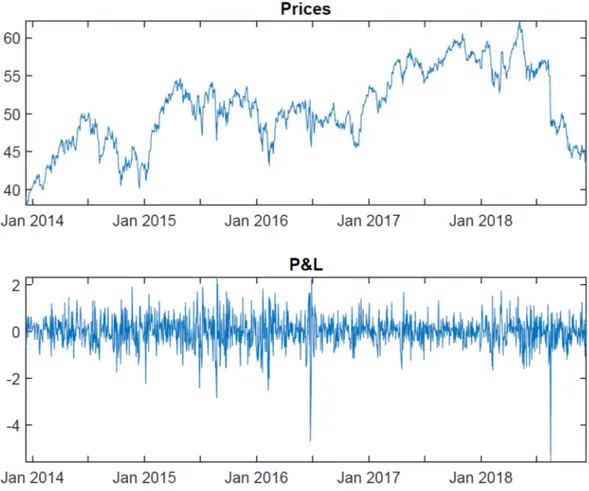
∑>O?@ O ; that is, we buy one unit of each stock. Figure 1 shows the dynamics of portfolio prices and of the P&L; some descriptive statistics of the P&L of the stocks and of the portfolio are reported in Table 1.
7
Figure 1: Daily portfolio prices and P&L.
Looking at Figure 1 we notice some high peaks followed by a drop, this shows high volatility of data; to be more precise, we analyze Table 1.
ATL BRE ENI ISP TIT Port
Mean 0.0011 0.0045 -0.0023 0.0002 -0.0001 0.0034 St Dev 0.3683 0.1618 0.2291 0.0547 0.0188 0.6538 Min -5.2400 -0.7440 -1.3400 -0.5180 -0.1375 -5.5933 Max 1.3000 0.8840 0.8500 0.3100 0.1010 2.3360 Skew -2.3574 0.2630 -0.2875 -0.5681 -0.0890 -0.8073 Kurt 36.3471 6.0586 5.3169 11.1909 6.9823 9.8177
Table 1: Daily P&L descriptive statistics.
The means are close to zero, in particular for Intesa and Telecom. This is reasonable since we consider one-day P&Ls. Standard deviations and ranges1 confirm high volatility of the portfolio P&L, since the first three stocks have a high standard deviation. Skewness is positive for Brembo, while it is negative for the others and far from zero for Atlantia. Kurtosis is very high, in particular for
8 Atlantia: this can be also seen from the minimum P&L which Atlantia performed in the considered period. Skewness and Kurtosis highlight how the data are far from being normally distributed, taking into account that Normal distribution has zero Skewness and Kurtosis equal 3. Rather, they seem to come from heavy-tailed distributions. In such situations, therefore, it may happen that VaR does not encourage diversification of risk.
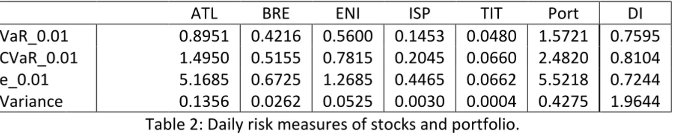
We apply the considered risk measures to each stock and to the whole portfolio, using the historical simulation method (see for instance Jorion [12]); that is, we replace the theoretical distribution of the P&L with the observed time series and we compute risk measures using these data. To illustrate the procedure we show how we compute historical VaR, i.e. how we sample the empirical quantile. We take each time series and sort the data concerning daily P&Ls from the smallest to the largest, then we assign to each price a weight of 1/1268, where 1268 is the number of observed daily P&Ls. We compute the empirical cumulative distribution function by computing cumulative weights: starting from the smallest P&L, we sum the weight of the previous P&L to the weight of the current one, until the last observed P&L. Then we set α=0.01 and we look for the smallest value which has a cumulative weight greater than 0.01; changing the sign of this value, we obtain VaR at the level 0.01. We compute in a similar way the other risk measures, letting α=0.01; this means, for the entropic risk measure, a high risk aversion and so a more conservative risk measure. We also compute the diversification index, given by Equation (10), for each risk measure. The results we obtained are shown in Table 2.
ATL BRE ENI ISP TIT Port DI
VaR_0.01 0.8951 0.4216 0.5600 0.1453 0.0480 1.5721 0.7595
CVaR_0.01 1.4950 0.5155 0.7815 0.2045 0.0660 2.4820 0.8104
e_0.01 5.1685 0.6725 1.2685 0.4465 0.0662 5.5218 0.7244
Variance 0.1356 0.0262 0.0525 0.0030 0.0004 0.4275 1.9644
Table 2: Daily risk measures of stocks and portfolio.
Looking at Table 2 we notice that the entropic risk measure is the most conservative one; this is due to the small value we set, as we explained before. A diversification effect is obtained for the first three risk measures, despite VaR and the entropic risk measure are, in general, not subadditive. We check this simply by looking at the diversification index: the first three risk measures have a DI less than 1, hence they are subadditive in this example. In particular, the entropic risk measure obtained the highest diversification effect. The diversification effect is not achieved from the variance, which is super-additive in this example, in fact it has a diversification index greater than 1.
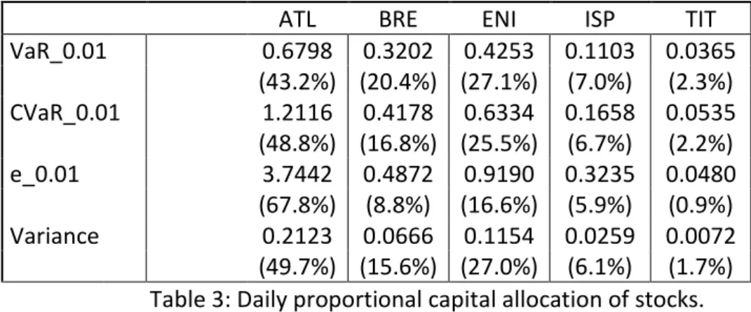
9 We compute the risk capital allocated to each stock, using the proportional methods presented in the previous section; the results are shown in Table 3.
ATL BRE ENI ISP TIT
VaR_0.01 0.6798 0.3202 0.4253 0.1103 0.0365 (43.2%) (20.4%) (27.1%) (7.0%) (2.3%) CVaR_0.01 1.2116 0.4178 0.6334 0.1658 0.0535 (48.8%) (16.8%) (25.5%) (6.7%) (2.2%) e_0.01 3.7442 0.4872 0.9190 0.3235 0.0480 (67.8%) (8.8%) (16.6%) (5.9%) (0.9%) Variance 0.2123 0.0666 0.1154 0.0259 0.0072 (49.7%) (15.6%) (27.0%) (6.1%) (1.7%)
Table 3: Daily proportional capital allocation of stocks.
Looking at Table 3 we notice that, for the first three capital allocation methods the risk capital allocated to each stock considered as an element of the portfolio does not exceed the risk capital allocated to the stock considered as a stand-alone portfolio. To check this, we simply compare the results of Table 3 to the results of Table 2; since each value of the first three rows of Table 3 is less than the respective value of Table 2, the pooling effect mentioned above is obtained. This follows straightforwardly from the diversification effect we obtained in Table 2: as on our data the considered risk measures turn out to behave subadditively and as ρ(Xi)≥0 for all i, Equation (7) shows that risk
capitals allocated via proportional allocation methods benefit of the pooling effect. In particular, the proportional method based on the entropic risk measure has benefited from the highest pooling effect. The reason is clear, since the entropic risk measure has the highest diversification index and the proportional methods allocate the capital via B= = JKC∙ ρ = , the allocated capital by using the entropic risk measure is, for each unit of risk capital ρ(Xi), less than the capital allocated via
proportional methods based on different risk measures. Since variance is superadditive in this example, the pooling effect is not obtained from this risk measure and the risk capital allocated to each stock considered as an element of the portfolio exceeds the risk capital allocated to the stock considered as a stand-alone portfolio. The full allocation property is satisfied for each risk measure: summing by row the values in Table 3 we obtain exactly the last column of Table 2; that is, the sum of risk capitals allocated to each stock is equal to the risk capital allocated to the portfolio using the respective risk measure. Furthermore, the results of Table 3 show also that all the capital allocation rules here considered agree in putting more weight on Atlantia than on others, reflecting the large risk capital assigned to this single stock. Moreover, also the ranking of capital allocation weights across the different sub-units is more or less the same for all the different rules that have been considered.
10 So far, we have considered proportional capital allocations using VaR, CVaR, the entropic risk measure and covariance. We investigate now what happens with marginal or RORAC methods and we compare the results with those of proportional methods. A priori we could expect that the marginal method would distribute differently the capital to be allocated by putting more weight on the riskier assets.
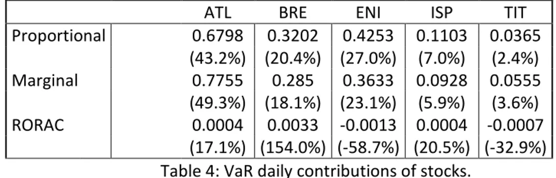
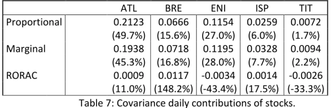
Here below (see tables 4, 5, 6 and 7) we present the results obtained by computing the risk capital allocated to each stock, via marginal methods and the contribution of stocks to the total portfolio RORAC. Each table reports the risk capital allocated to each stock using both proportional methods and marginal ones and the contribution of each stock to the total portfolio RORAC, for any single risk measure. For what concerns the contribution to the total RORAC, we compute the contributions of stocks by using just the proportional allocation methods.
ATL BRE ENI ISP TIT
Proportional 0.6798 0.3202 0.4253 0.1103 0.0365 (43.2%) (20.4%) (27.0%) (7.0%) (2.4%) Marginal 0.7755 0.285 0.3633 0.0928 0.0555 (49.3%) (18.1%) (23.1%) (5.9%) (3.6%) RORAC 0.0004 0.0033 -0.0013 0.0004 -0.0007 (17.1%) (154.0%) (-58.7%) (20.5%) (-32.9%)
Table 4: VaR daily contributions of stocks.
ATL BRE ENI ISP TIT
Proportional 1.2116 0.4178 0.6334 0.1658 0.0535 (48.8%) (16.8%) (25.5%) (6.7%) (2.2%) Marginal 1.3998 0.2518 0.614 0.1651 0.0514 (56.4%) (10.1%) (24.7%) (6.7%) (2.1%) RORAC 0.0002 0.002 -0.0007 0.0002 -0.0004 (12.1%) (148.6%) (-49.7%) (17.2%) (-28.2%)
Table 5: CVaR daily contributions of stocks.
ATL BRE ENI ISP TIT
Proportional 3.7442 0.4872 0.9190 0.3235 0.0480 (67.8%) (8.8%) (16.6%) (5.9%) (0.9%) Marginal 4.9476 0.1788 0.3283 0.0658 0.0013 (89.6%) (3.2%) (6.0%) (1.1%) (0.1%) RORAC 0.0000 0.0010 -0.0003 0.0001 -0.0003 (5.3%) (171.2%) (-46.0%) (11.8%) (-42.3%)
11
ATL BRE ENI ISP TIT
Proportional 0.2123 0.0666 0.1154 0.0259 0.0072 (49.7%) (15.6%) (27.0%) (6.0%) (1.7%) Marginal 0.1938 0.0718 0.1195 0.0328 0.0094 (45.3%) (16.8%) (28.0%) (7.7%) (2.2%) RORAC 0.0009 0.0117 -0.0034 0.0014 -0.0026 (11.0%) (148.2%) (-43.4%) (17.5%) (-33.3%)
Table 7: Covariance daily contributions of stocks.
Looking at Tables 4, 5, 6 and 7 we notice not too significant differences between the proportional methods and the marginal one: among different risk measures, both methods agree in putting more weight on Atlantia than on others and the ranking of capital allocation weights across the different stocks is the same for both methods. Nevertheless, apart from the case of covariance that however is not really a risk measure, it is worth to emphasize that our “intuition” concerning marginal contributions was correct. Compared to proportional capital allocations, indeed, marginal contributions put more weight (in terms of capital allocation) on Atlantia that is the riskiest asset in the portfolio. Among different risk measures, the ranking of the contributions to the total RORAC is still the same: Brembo gives the best contribution, which is even more than the total RORAC, and Eni gives the worst contribution, which is negative; i.e. it is not worth having such an asset in the portfolio, since it reduces the total RORAC. Risk capitals allocated via marginal methods benefit of the pooling effect for the first three risk measures, except the capital allocated to Telecom using VaR: this amount is larger than VaR of Telecom considered as a stand-alone portfolio. As well as for proportional methods, the marginal method based on the entropic risk measure has benefited from the highest pooling effect. Despite this result it is not evident from marginal methods' formula, the data confirm: comparing the values of Table 2 with those of Tables 4, 5 and 6 we can notice that the marginal method based on the entropic risk measure has the highest difference between the risk capital of the titles and the capital allocated to them by using this method. The pooling effect is not achieved by the covariance marginal allocation method, as well as for the proportional one, as we noted above. The full allocation property for marginal allocation methods is, of course, satisfied for each risk measure since we use the adjusted formulation in (9). By the same argument, the sum of RORAC contributions is equal to the total portfolio RORAC, for each risk measure.
4
Conclusions
In the present work we have revised a problem which is very popular in the financial literature, namely the one of Capital Allocation. This problem can be faced in many ways, as it is evident from the huge literature on the subject ([16] gives a complete overview), but one of the most known is the
12 one illustrated in this work, that is through the use of risk measures. Namely, for a given risky financial activity X composed by n sub-units X1, …, Xn, whose riskiness is covered through a capital
requirement assessed by a risk measure ρ, the problem consists in suitably sharing the risk capital
ρ(X) among the business units, in such a way that the capital is fully allocated and that a diversification effect is obtained. The possibility of verifying these properties depends both on the chosen risk measure and on the Capital Allocation method. In this short paper, we have applied two well known Capital Allocation methods (the proportional and the marginal one) to a portfolio of stocks whose capital requirements are determined through three of the most used risk measures: Value at Risk, Conditional Value at Risk and the entropic risk measure, and we have compared and discussed the results obtained. Based on the numerical example above, we cannot conclude that a given capital allocation method is always better than another. However, for the risk measures examined the results obtained by proportional and marginal methods are substantially very different from those of the RORAC method. Even if proportional and marginal contribution methods seem to provide similar results, marginal one better reacts and takes into account riskier assets.
References
[1]Acerbi, C., Tasche, D. (2002). On the coherence of expected shortfall. Journal of Banking and Finance, 26(7), 1487-1503.
[2]Artzner, P., Delbaen, F., Eber, J. M., Heath, D. (1997): Thinking Coherently, RISK 10, 68-71.
[3]Artzner, P., Delbaen, F., Eber, J. M., Heath, D. (1999). Coherent measures of risk. Mathematical Finance, 9(3), 203-228.
[4]Barrieu, P., El Karoui, N. (2009): Pricing, hedging and optimally designing derivatives via minimization of risk measures. In: Volume on Indifference Pricing (ed. René Carmona), Princeton University Press.
[5] Basle Committee (1996): Amendment to the Capital Accord to Incorporate Market Risks. Basle Committee on Banking Supervision.
[6] Basel Committee on Banking Supervision (2017-2018): Basel III Monitoring Report.
[7] Centrone, F., Rosazza Gianin, E. (2018). Capital allocation à la Aumann-Shapley for non-differentiable risk measures. European Journal of Operational Research, 267(2), 667-675. [8] Denault, M. (2001). Coherent allocation of risk capital. Journal of Risk 4/1, 1-34.
[9] Dhaene, J., Tsanakas, A., Valdez, E. A., Vanduffel, S. (2012). Optimal capital allocation principles. Journal of Risk and Insurance, 79(1), 1-28.
[10] Föllmer, H., Schied, A. (2016). Stochastic Finance: an introduction in discrete time. Walter de Gruyter. Fourth edition.
13 [11] Frittelli, M., Rosazza Gianin, E. (2002). Putting order in risk measures. Journal of
Banking and Finance, 26(7), 1473-1486.
[12] Jorion, P. (1997). Value at risk: the new benchmark for controlling market risk. Irwin Professional Pub.
[13] Kalkbrener, M. (2005). An axiomatic approach to capital allocation. Mathematical Finance, 15/3, 425-437.
[14] Rockafellar, R. T., Uryasev, S. (2002). Conditional value-at-risk for general loss distributions. Journal of banking and finance, 26(7), 1443-1471.
[15] Tasche, D. (2004). Allocating portfolio economic capital to subportfolios. Economic capital: a practitioner guide, 275-302.
[16] Vener, G.G. (2004). Capital allocation survey with commentary. North American Actuarial Journal, 8(2), 96-107.