SOME RESULTS ON NON-CENTRAL BETA DISTRIBUTIONS
Andrea Ongaro
Dipartimento di Economia, Metodi Quantitativi e Strategie di Impresa, Universit`a degli Studi di Milano-Bicocca, Via Bicocca degli Arcimboldi 8, 20126 Milano, Italia
Carlo Orsi1
Dipartimento di Economia, Metodi Quantitativi e Strategie di Impresa, Universit`a degli Studi di Milano-Bicocca, Via Bicocca degli Arcimboldi 8, 20126 Milano, Italia
1. Introduction
The beta distribution plays a central role in modeling a wide variety of random phenomena which can take on values with lower and upper bounds. For example, such distribution has been employed to model the time to perform an activity in the project management area (Malcolm et al., 1959) and has been used to fit the sample distribution of soil parameters (Haskett et al., 1995). In particular, the beta distribution is useful for modeling propor-tions. Such distribution, in fact, has been applied to fit the monthly frequency distribution of the daily sunshine duration measurements collected at various locations in Algeria (Et-toumi et al., 2002) and has been employed to model heterogeneity in the probability of HIV transmission per sexual contact (Wiley et al., 1989).
Therefore, the beta distribution is versatile enough to model different types of data. Despite this, several generalizations of such distribution have been developed in order to achieve further flexibility. In this regard, see Johnson et al. (1995) and McDonald and Xu (1995). However, neither the beta distribution nor the major part of its generalizations offer flexibility to the limits at 0 and 1 of their probability density functions. On the contrary, the class of the so-called “non-central” beta distributions display such behavior which, to our knowledge, has never been studied. Such class, however, is affected by strong limitations in terms of tractability and interpretability.
That said, in this paper we shall introduce a new distribution on the real interval (0, 1) which can be viewed as a more easily tractable and interpretable analogue of the doubly non-central beta distribution (Johnson et al., 1995). More specifically, the present paper is organized as follows. In Section 2 some notations are introduced and some useful facts are recalled. Particular attention is focused on the non-central chi-squared distribution, which plays a crucial role in the study of the family of the generalizations of the beta distribution we are interested in. In Section 3 we shall provide a novel analysis of the standard non-central beta distribution. In particular, the perturbation representation of such distribution highlights its uneasy tractability and interpretability. In Section 4 we shall perform a preliminary investigation of the properties of a new non-central beta distribution. The analysis of such distribution is based on the same techniques employed in the study of the standard one and will allow a better understanding of the similarities and differences between the two distributions.
1
2. Preliminaries
It is well known that if Yi, i = 1, 2, are independent χ2 random variables with 2αi > 0
degrees of freedom, denoted by χ22αi, then the random variable:
X = Y1 Y1+ Y2
(1) has a beta distribution with shape parameters αi, denoted by Beta(α1, α2). Its density is:
Beta (x; α1, α2) =x
α1−1 (1− x)α2−1
B (α1, α2)
, 0 < x < 1 . (2)
The beta distribution can also be obtained as conditional distribution of X given the sum Y+ = Y
1+ Y2, as a consequence of the independence of X and Y+. The latter is a characterizing property of (independent) gamma random variables.
Let us now recall the definition and some useful properties of the non-central chi-squared distribution, which plays a crucial role in the study of the family of the generalizations of the beta distribution we are interested in.
Let Wk, k = 1, . . . , g, be independent and normally distributed random variables with
means µk and unitary variances. Then, a random variable is said to have a non-central
chi-squared distribution with g > 0 degrees of freedom and non-centrality parameter λ = ∑g
k=1µ
2
k≥ 0, denoted by χ′ 2g (λ), if it is distributed as:
Y′ =
g
∑
k=1
Wk2
(Johnson et al., 1995). The case λ = 0 corresponds to the χ2
g distribution.
The density function fY′ of Y′∼ χ′ 2g (λ) can be expressed as:
fY′(y; g, λ) = +∞ ∑ i=0 e−λ2 (λ 2 )i i! yg+2i2 −1e− y 2 Γ(g+2i2 )2g+2i2 , y > 0, (3)
i.e. as series of the χ2
g+2i densities,∀i ∈ N ∪ {0}, weighted by the probabilities of a Poisson
random variable with mean λ/2, λ≥ 0 (the case λ = 0 corresponding to a random variable degenerate at zero).
In view of Eq. (3), the χ′ 2g (λ) distribution admits the following mixture representation. Proposition 1 (Mixture representation). Let Y′ have a χ′ 2g (λ) distribution and
M be a Poisson random variable with mean λ/2. Then, Y′ admits the following representa-tion:
Y′| (M = i) ∼ χ2g+2i. (4)
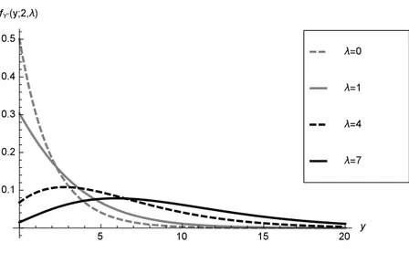
The χ′ 2g (λ) density can assume a larger variety of shapes than the central one. In
particular, the limit at 0 of such density is decreasing in λ when g = 2.
Proposition 2 (Limit at 0 of the χ′ 2g (λ) density when g = 2). Let Y′be a χ′ 2g (λ)
random variable with g = 2 and λ≥ 0. Let fY′ be the density of Y′. Then:
lim y→0+fY ′(y; 2, λ) =1 2e −λ 2. (5)
In this regard, see Figure 1.
Finally, we recall that the non-central chi-squared distribution is reproductive with re-spect to both degrees of freedom and non-centrality parameter.
Figure 1 – Plots of the density of Y′∼ χ′ 2g (λ) for g = 2 and selected values of λ.
Proposition 3 (Reproductive property). If Yj′, j = 1, . . . , m, are independent
with χ′2gj(λj) distributions, then:
Y′+= m ∑ j=1 Yj′ ∼ χ′2g(λ), where g =∑mj=1gj and λ = ∑m j=1λj.
Such property can be easily derived from its characteristic function (Johnson et al., 1995).
3. The standard non-central beta distribution
Let us now recall the definition and some useful representations of the standard non-central beta distribution.
Let Yi′, i = 1, 2, be independent χ′ 22α
i(λi) random variables. Then, a random variable
is said to have a doubly non-central beta distribution with shape parameters α1, α2 and non-centrality parameters λ1, λ2, denoted by DNCB (α1, α2, λ1, λ2), if it is distributed as
X′ = Y
′
1
Y1′+ Y2′ (6)
(Johnson et al., 1995).
The DNCB density can be easily derived by using the mixture representation of the non-central χ2 distribution. Specifically, let M
i, i = 1, 2, be independent Poisson random
variables with means λi/2. Conditionally on (M1, M2), X′has a Beta(α1+M1, α2+M2) dis-tribution, Yi′|(M1, M2) being independent with distributions χ22αi+2Mi, i = 1, 2. Therefore,
the density function fX′ of X′ ∼ DNCB (α1, α2, λ1, λ2) can be expressed as:
fX′(x; α1, α2, λ1, λ2) = +∞ ∑ j=0 +∞ ∑ k=0 e−λ12 (λ1 2 )j j! e−λ22 (λ2 2 )k k! xα1+j−1(1− x)α2+k−1 B (α1+ j, α2+ k) , 0 < x < 1, (7) i.e. as double series of the Beta(α1+ j, α2+ k) densities, ∀j, k ∈ N ∪ {0}, weighted by the joint probabilities of the bivariate random variable (M1, M2), where Mi, ∀i = 1, 2, are
independent with Poisson (λi/2) distributions.
Proposition 4 (Mixture representation). Let X′have a DNCB (α1, α2, λ1, λ2)
dis-tribution. Then, X′ admits the following representation:
X′| (M1= j, M2= k)∼ Beta (α1+ j, α2+ k) , (8)
where Mi, i = 1, 2, are independent Poisson random variables with means λi/2.
The perturbation representation of the doubly non-central beta distribution highlights the uneasy tractability and interpretability of such distribution.
Proposition 5 (Perturbation representation). Let X′ ∼ DNCB (α1, α2, λ1, λ2).
Then, the density fX′ of X′ can be written as:
fX′(x; α1, α2, λ1, λ2) = Beta (x; α1, α2)· e− λ+ 2 Ψ2 [ α+; α1, α2;λ1 2 x, λ2 2 (1− x) ] , (9) where α+= α 1+ α2, λ+= λ1+ λ2, Ψ2[α; γ, γ′; x, y] = +∞ ∑ j=0 +∞ ∑ k=0 (α)j+k (γ)j(γ′)k xj j! yk k!, x, y≥ 0 (10)
is the Humbert’s confluent hypergeometric function (Srivastava and Karlsson, 1985) and
(a)0= 1, (a)i = a (a + 1) . . . (a + i− 1) , ∀i ∈ N (11)
is the Pochhammer’s symbol or ascendent factorial.
The perturbing factor of the beta density in the doubly non-central beta distribution is a function in two variables given by the sum of a double power series (Eq. (10)). Such function has not a simple behavior and, to our knowledge, is not reducible to a more tractable analytical form. Therefore, it’s not easy to understand the effect of such factor.
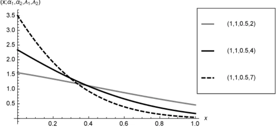
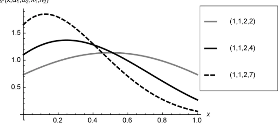
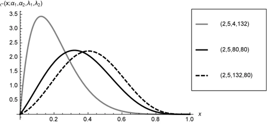
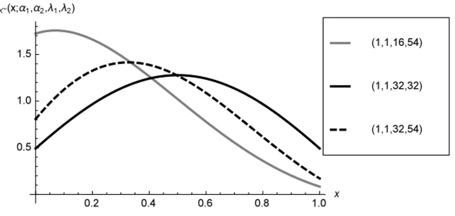
Despite this, the DNCB density can assume a large variety of shapes far beyond the beta model ones. In this regard, Figures 2, 3, 4, 5, 6 display the DNCB density for selected values of the parameters. In particular, the effect of the perturbing factor can be clearly seen when α1 = α2 = 1, because in this case the beta density reduces to the uniform one (see Figures 4, 5, 6).
Figure 2 – Plots of the density of X′∼ DNCB (α1, α2, λ1, λ2) for selected values of (α1, α2, λ1, λ2).
Moreover, it is well known that the limits at 0 and 1 of the beta density are equal to 0 or +∞ if αi̸= 1 and are equal to 1 if αi= 1, i = 1, 2. When αi ̸= 1 the DNCB density shows
the same limiting characteristics as the beta model ones. On the contrary, when αi= 1 the
doubly non-central beta density shows the attractive feature of taking on arbitrary finite and positive limits at 0 and 1. To our knowledge, such characteristic of the DNCB density has never been studied. More specifically, such limits have the following expressions.
Figure 3 – Plots of the density of X′∼ DNCB (α1, α2, λ1, λ2) for selected values of (α1, α2, λ1, λ2).
Figure 4 – Plots of the density of X′∼ DNCB (α1, α2, λ1, λ2) for α1= α2= 1 and selected values of λ1, λ2.
Remark 6 (Limits at 0 and 1 of the DNCB density when α1= α2= 1). Let X′
∼ DNCB (α1, α2, λ1, λ2). Then, the limits at 0 and 1 of the density fX′(α1, α2, λ1, λ2) of
X′ when α1= α2= 1 are: lim x→0+fX′(x; 1, 1, λ1, λ2) = e −λ1 2 ( λ2 2 + 1 ) , (12) lim x→1− fX′(x; 1, 1, λ1, λ2) = e− λ2 2 ( λ1 2 + 1 ) . (13)
Notice that, under the case of unitary shape parameters, the limit at 0 of the DNCB density is increasing in λ2 for any fixed λ1> 0 and decreasing in λ1 for any fixed λ2> 0, while the limit at 1 is decreasing in λ2 for any fixed λ1> 0 and increasing in λ1 for any fixed λ2> 0. Finally, by exploiting the mixture representation in Eq. (8), it is possible to derive a new general formula for the moments of the standard non-central beta distribution. Specifically, the moments of the DNCB distribution can be written and represented as follows.
Proposition 7 (Moments). Let X′ ∼ DNCB (α1, α2, λ1, λ2). Let Mj, j = 1, 2, be
independent Poisson random variables with means λj/2 and M+= M1+M2. Then,∀r ∈ N,
the r-th moment of X′ can be written as:
E[(X′)r| M+]= 1 (α++ M+) r M+ ∑ i=0 (α1+ i)r ( M+ i ) ( λ1 λ+ )i ( 1− λ1 λ+ )M+−i (14)
Figure 5 – Plots of the density of X′∼ DNCB (α1, α2, λ1, λ2) for α1= α2= 1 and selected values of λ1, λ2.
Figure 6 – Plots of the density of X′∼ DNCB (α1, α2, λ1, λ2) for α1= α2= 1 and selected values of λ1, λ2.
and admits the following representation:
E[(X′)r]=E(M1,M2) [ (α1+ M1)r (α++ M+) r ] . (15)
Proof. Observe first that, in the notation of Eq. (6), Y′+= Y1′+ Y2′ and X′ = Y1′/Y′+ are independent conditionally on M+. In this regard, notice that Eq. (8) can be rewritten as follows: X′|(M1, M+ ) ∼ Beta(α1+ M1, α2+ M+− M1 ) ; (16)
similarly, since Y′+∼ χ′22α+(λ+) in view of Proposition 3, Eq. (4) can be rewritten as follows:
Y′+ (M1, M+ ) d
= Y′+ M+∼ χ22α++2M+. (17)
Therefore, X′ and Y′+ are conditionally independent given (M1, M+), the latter being a characterizing property of independent gamma random variables. Hence, conditionally on (M1, M+), the joint distribution of (X′, Y′+) factorizes into the marginal distributions of
X′ and Y′+. Finally, the joint density function of (X′, Y′+)| M+ turns out to factorize into the marginal density functions of X′|M+ and Y′+|M+. Indeed, by recalling that
M1|M+∼ Binomial (
M+,λ1
λ+
)
, one can obtain:
f(X′,Y′+)|M+(x, y) = M+ ∑ i=0 Pr(M1= i| M+ ) · f(X′,Y′+)|(M1,M+)(x, y) = = fY′+|M+(y)· fX′|M+(x) , where: fX′|M+(x) = M+ ∑ i=0 Binomial ( i; M+, λ1 λ+ ) · Beta(x; α1+ i, α2+ M+− i ) , with: Binomial ( i; M+, λ1 λ+ ) = ( M+ i ) ( λ1 λ+ )i ( 1− λ1 λ+ )M+−i , i = 0, . . . , M+.
That said, because of the foregoing arguments, the following holds: E[(X′)r M+]= E
[
(Y1′)r M+]
E [(Y′+)r| M+
], (18)
where, in view of the general formula for the moments of the gamma distribution (Johnson
et al., 1994): E[(Y1′)r M+]=E[2r(α1+ M1)r| M+]= 2r M+ ∑ i=0 (α1+ i)r ( M+ i ) ( λ1 λ+ )i( 1− λ1 λ+ )M+−i (19) and: E[(Y′+)r M+]= 2r (α++ M+)r. (20) Hence, Eq. (14) is established.
Finally, by letting L∼ Binomial (M+, λ
1/λ+) in Eq. (14), one can obtain that: E[(X′)r M+]= E [(α1+ L)r]
(α++ M+)
r
. (21)
Thus, in view of the fact that L= M1d | M+, Eq. (15) is established. 2 The formula in Eq. (14) reduces the computation of moments of the DNCB distribution from a double series to a single one. In particular, by setting r = 1 and r = 2 and after some manipulations, the first two moments of the DNCB distribution can be written in terms of perturbations of the corresponding moments of the beta distribution as follows:
E (X′) = α1 α+e −λ+ 2 [ 1F1 ( α+; α++ 1;λ + 2 ) + α + λ1 2 α1(α++ 1) 1F1 ( α++ 1; α++ 2;λ + 2 )] , (22) E[(X′)2 ] = (α1)2 (α+) 2 e−λ+2 [ 1F1 ( α+; α++ 2;λ + 2 ) + α +λ 1 α1(α++ 2)· · 1F1 ( α++ 1; α++ 3;λ + 2 ) + (α +) 2 (λ1 2 )2 (α1)2(α++ 2)2 1F1 ( α++ 2; α++ 4;λ + 2 )] , (23) where: 1F1(a; b; x) = +∞ ∑ i=0 (a)i (b)i xi i!, a, b > 0, x≥ 0
is the generalized hypergeometric functionpFq with p = 1 and q = 1 coefficients respectively at numerator and denominator, otherwise known as Kummer’s confluent hypergeometric function (Srivastava and Karlsson, 1985).
4. A new non-central beta distribution
Our basic idea to introduce a new family of non-central beta distributions is to consider the conditional distribution of a DNCB random variable X′given Y1′+ Y2′, Yi′being independent with χ′ 22α
i(λi) distributions, i = 1, 2. Because of the above mentioned characterizing
prop-erty of independent gamma random variables, such conditional distribution must depend on
Y1′+ Y2′ and therefore must be different from the DNCB distribution, unless λ1= λ2= 0. The latter case corresponds to the beta distribution.
The density of the new non-central beta distribution can be derived by using the mix-ture representation of the non-central χ2 distribution. Specifically, let Mi, i = 1, 2, be
independent Poisson random variables with means λi/2. Conditionally on (M1, M2), X′ =
Y1′/(Y1′+ Y2′) and Y1′+ Y2′ are independent; therefore, X′ given (M1, M2, Y1′ + Y2′) has a Beta(α1+ M1, α2+ M2) distribution. A direct application of Bayes’ theorem then shows that, conditionally on Y1′+ Y2′ = y, for any fixed y > 0, (M1, M2) has the following joint probability function: Pr (M1= j, M2= k| Y1′+ Y2′= y) = 1 0F1 ( α+,y λ+ 4 ) ( y λ1 4 )j ( y λ2 4 )k j! k! (α+) j+k , j, k∈ N ∪ {0}, (24) where 0F1(a; x) = +∞ ∑ i=0 1 (a)i xi i!, a > 0, x≥ 0 (25)
is the generalized hypergeometric functionpFq with p = 0 and q = 1 coefficients respectively at numerator and denominator (Srivastava and Karlsson, 1985).
As the conditioning value y in Eq. (24) can be incorporated in the non-centrality parame-ters λi’s, we are then led to the following definition of the above mentioned new distribution.
Definition 8. A random variable is said to have a conditional doubly non-central beta
distribution with shape parameters α1, α2 and non-centrality parameters λ1, λ2, denoted by CDNCB (α1, α2, λ1, λ2), if it is distributed as X′′= Y ′ 1 Y1′+ Y2′ Y′ 1+ Y2′= 1 (26)
where Yi′, i = 1, 2, are independent χ′ 22α
i(λi) random variables. The random variable in
Eq. (26) is meant to be distributed according to the regular version of the conditional density of Y1′|Y1′ + Y2′ = 1 which is proportional to the product of the densities of Y1′ and Y2′ respectively evaluated in x and 1− x.
By mixturing the density function of X′ given (M1, M2, Y1′+ Y2′= 1) with respect to the joint probability function of (M1, M2) given Y1′+ Y2′ = 1, one can obtain the density function
fX′′ of X′′∼ CDNCB (α1, α2, λ1, λ2) which turns out to have the following expression:
fX′′(x; α1, α2, λ1, λ2) = +∞ ∑ j=0 +∞ ∑ k=0 (λ1 4) j (λ2 4) k j! k! (α+)j+k 0F1 ( α+,λ+ 4 )xα1+j−1(1− x) α2+k−1 B (α1+ j, α2+ k) , 0 < x < 1, (27)
given by the double series of the Beta(α1+ j, α2+ k) densities,∀j, k ∈ N ∪ {0}, weighted by the joint probabilities of the bivariate random variable (N1, N2), whose probability function is given by Eq. (24) with y = 1. The above discussion directly leads to the following mixture representation.
Proposition 9 (Mixture representation). Let X′′ have a CDNCB (α1, α2, λ1, λ2)
distribution. Then, X′′ admits the following representation:
X′′| (N1= j, N2= k)∼ Beta (α1+ j, α2+ k) , (28)
where the joint probability function of (N1, N2) is given by Eq. (24) with y = 1.
Although the distribution of (N1, N2) is slightly more complicated than the one of (M1, M2), it can be easily handled and understood in terms of the random variables (N1, N+), where N+= N1+ N2 has the following probability function:
Pr(N+= i)= 1 0F1 ( α+;λ+ 4 ) 1 (α+) i ( λ+ 4 )i i! , i∈ N ∪ {0} . (29)
Interestingly, N1| N+ shares the same distribution of M1|M+, with M+= M1+ M2. More specifically, the following holds true.
Remark 10. Let (N1, N2) be jointly distributed as in Eq. (24) with y = 1 and N+ =
N1+ N2 be distributed as in Eq. (29). Then:
Ni| N+∼ Binomial ( N+, λi λ+ ) , i = 1, 2. (30)
This allows us to derive the expression for the covariance between N1and N2 as follows: Cov (N1, N2) = EN+ { Cov[(N1, N2)|N+]}+ Cov[E(N1|N+ ) ,E(N2|N+ )] = = λ1λ2 (λ+)2 [ Var(N+)− E(N+)] , (31)
which can be easily expressed in terms of the hypergeometric function 0F1. An extensive numerical investigation shows that such covariance is negative.
It is also simple to check that the CDNCB admits an unconditional “ratio” type repre-sentation.
Remark 11 (Ratio representation). Let (N1, N2) be jointly distributed as in Eq. (24)
with y = 1. Let (Z1, Z2) be conditionally independent random variables given (N1, N2), with
Zi| (N1, N2)∼ χ2α2 i+2Ni, i = 1, 2. Then:
Z1
Z1+ Z2 ∼ CDNCB (α
1, α2, λ1, λ2) . (32)
Notice that (Z1, Z2) are negatively correlated as Cov (Z1, Z2) = 4 Cov (N1, N2).
The CDNCB model can be easily simulated by using either its mixture or ratio represen-tations. In both cases it’s necessary to simulate the joint distribution of (N1, N2). Such issue can be addressed by first generating the random variable N+ in Eq. (29) and then N
1|N+ in Eq. (30). As the former distribution is similar to the Poisson one, it can be simulated by using, for example, the inverse-transform method (see e.g. Law and Kelton, 2000).
To fully understand the behavior of the new non-central beta distribution it is instructive to realize how it perturbates the beta one.
Proposition 12 (Perturbation representation). Let X′′∼ CDNCB (α1, α2, λ1, λ2).
Then the density fX′′ of X′′ can be written as:
fX′′(x; α1, α2, λ1, λ2) = Beta(x; α1, α2)· 0F1 ( α1;λ1x 4 ) 0F1 [ α2;λ2(1−x) 4 ] 0F1 ( α+;λ+ 4 ) . (33)
Proof. Observe that Eq. (11) is tantamount to: (a)i= Γ (a + i)
Γ (a) , ∀i ∈ N ∪ {0}, (34)
where Γ (·) is the gamma function.
In the light of Eq. (34) and in the notation of Eq. (27), one can obtain:
B (α1+ j, α2+ k) = Γ (α1) (α1)j Γ (α2) (α2)k Γ (α+) (α+) j+k = B (α1, α2) (α1)j (α2)k (α+) j+k .
Hence, by means of easy manipulations, Eq. (27) can be rewritten as follows:
fX′′(x; α1, α2, λ1, λ2) = Beta (x; α1, α2)· ∑+∞ j=0 (λ1 4x) j (α1)jj! ∑+∞ k=0 [λ2 4(1−x)] k (α2)kk! 0F1 ( α+;λ+ 4 ) .
Finally, by virtue of Eq. (25), Eq. (33) is established. 2
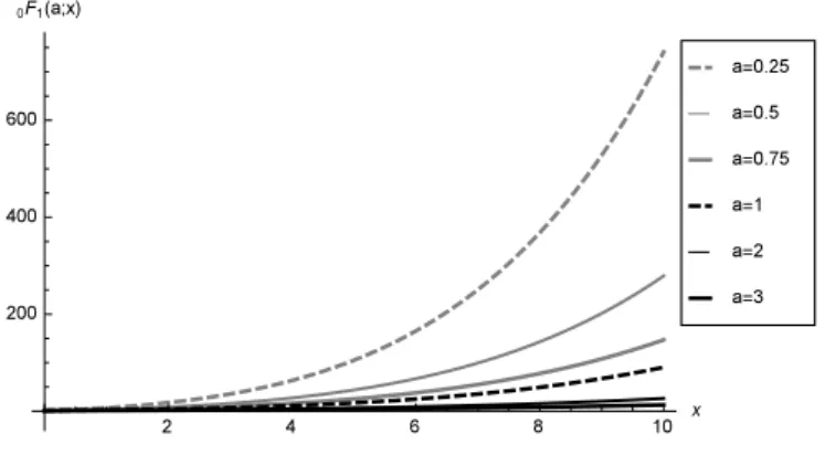
Such representation highlights the greater interpretability and tractability of the CDNCB distribution with respect to the DNCB. The perturbing factor of the beta density in the CDNCB distribution, unlike the DNCB one, has a product form involving only the 0F1 function (and therefore a single series) in a completely symmetric fashion. Furthermore, 0F1(a; x) has a very simple behavior and is implemented in common statistical packages. For any fixed a > 0, it is increasing, with values in [1, +∞) and convex. For fixed x ≥ 0, 0F1(a; x) and its first derivative with respect to x are decreasing in a. See plots in Figure 7.
Figure 7 – Plots of0F1(a; x) for x≥ 0 and selected values of a > 0.
It follows that 0F1(α1; λ1x/4) in Eq. (33) has the effect of giving more weight to the right tail of the beta density through the scale parameter λ1 and the shape parameter α1 determining the rate of increase of the function. Perfectly symmetric considerations hold for the other component0F1[α2; λ2(1− x) /4] of the perturbing factor.
That said, Figures 8, 9, 10, 11, 12 display the CDNCB density for selected values of the parameters. They show that such density assumes shapes similar to the DNCB ones.
However, in order to appreciate such a variety of shapes, the non-centrality parameters
λ1, λ2 have to be assigned higher values than the ones used to represent the DNCB density in Figures 2, 3, 4, 5 and 6. This discrepancy can be explained as follows.
The mixture representations given in Propositions 4 and 9 show that differences between the DNCB and the CDNCB can be entirely explained by differences between the distribu-tions of (M1, M2) and (N1, N2). The latter distributions, by Remark 10, share the same conditional distributions Ni|N+ and Mi|M+. It follows that differences between the DNCB
Figure 8 – Plots of the density of X′′∼ CDNCB (α1, α2, λ1, λ2) for selected values of (α1, α2, λ1, λ2).
Figure 9 – Plots of the density of X′′∼ CDNCB (α1, α2, λ1, λ2) for selected values of (α1, α2, λ1, λ2).
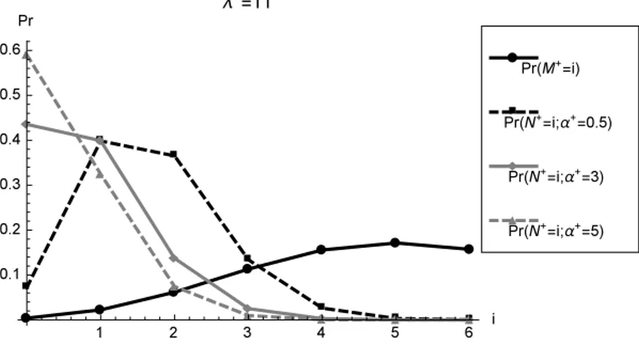
and the CDNCB are entirely due to differences between M+, which has a Poisson(λ+/2) distribution, and N+, with probability function given by Eq. (29). Some theoretical com-parisons between M+and N+ can be made by applying the following well known monotone likelihood ratio result. Suppose p1(i) and p2(i) are two probability functions corresponding to the random variables X1 and X2 respectively. Then a sufficient condition for X1 to be stochastically larger than X2 is that the likelihood ratio LR(i) = p1(i)/p2(i) is increasing (see, for example, Lehmann and Romano (2005), Lemma 3.4.2). A direct application of this result proves that N+ is stochastically smaller than M+, for any given α+> 1/2. Further-more, N+is stochastically decreasing in α+, for any given λ+, and stochastically increasing in λ+, for given α+. This explains why higher values of λ+ for the CDNCB are needed in order that its density resembles the DNCB one. It also indicates that this is even more so when α+ is large.
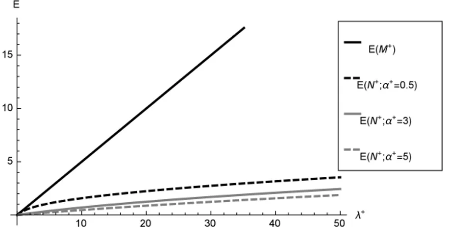
To appreciate the extent of this phenomenon, a graphical comparison of the probability functions of M+ and N+ for selected values of λ+ and of α+ is presented in Figures 13, 14 and 15. In particular, one can see that the discrepancy between the distributions of N+and
M+ increases when λ+ gets larger. A rough idea of the link between the λ+ values of the two distributions can be obtained by comparing their expected values. Figure 16 reports the plots of E(M+) = λ+/2 and of
E(N+) = λ+ 4 0F1 ( α++ 1;λ+ 4 ) α+ 0F1 ( α+;λ+ 4 )
Figure 10 – Plots of the density of X′′ ∼ CDNCB (α1, α2, λ1, λ2) for α1 = α2 = 1 and selected values of λ1, λ2.
Figure 11 – Plots of the density of X′′ ∼ CDNCB (α1, α2, λ1, λ2) for α1 = α2 = 1 and selected values of λ1, λ2.
as a function of λ+. From this plot, for a given value of E(M+) one can find the value λ+ relative to N+ which produces similar expectation. As expected, this λ+ value gets larger when α+ increases. It is also noticeable the strong increment of the difference between the two expectations for growing λ+.
As a further relevant property, the CDNCB density can take on arbitrary finite and positive limits at 0 and 1, as well as the DNCB (see Figures 10, 11 and 12). More specifically, such limits have the following expressions.
Remark 13 (Limits at 0 and 1 of the CDNCB density when α1= α2= 1). Let
X′′ ∼ CDNCB (α1, α2, λ1, λ2). Then, the limits of the density fX′′(α1, α2, λ1, λ2) of X′′ at 0 and 1 when α1= α2= 1 are:
lim x→0+fX′′(x; 1, 1, λ1, λ2) = 0F1 ( 1;λ2 4 ) 0F1 ( 2;λ+ 4 ), (35) lim x→1− fX′′(x; 1, 1, λ1, λ2) = 0 F1 ( 1;λ1 4 ) 0F1 ( 2;λ4+ ). (36)
Finally, notice that the general formulas for the moments of the DNCB distribution in Eq. (14) and (15) hold for the CDNCB distribution as well, provided we simply replace
Figure 12 – Plots of the density of X′′ ∼ CDNCB (α1, α2, λ1, λ2) for α1 = α2 = 1 and selected values of λ1, λ2.
Figure 13 – Probability functions of M+ and N+ for λ+= 1 and α+∈ {0.5, 3, 5}.
M+ by N+. Specifically, the moments of the CDNCB distribution can be written and represented as follows.
Proposition 14 (Moments). Let X′′have a CDNCB (α1, α2, λ1, λ2) distribution. Let (N1, N2) be jointly distributed as in Eq. (24) with y = 1 and N+= N1+ N2. Then,∀r ∈ N,
the r-th moment of X′′ can be written as:
E[(X′′)r| N+]= 1 (α++ N+) r N+ ∑ i=0 (α1+ i)r ( N+ i ) ( λ1 λ+ )i ( 1− λ1 λ+ )N+−i (37)
and admits the following representation:
E[(X′′)r]=E(N1,N2) [ (α1+ N1)r (α++ N+) r ] . (38)
Proof. The proof follows from arguments similar to those of Proposition 7 by making
use of the CDNCB ratio representation in Remark 11. 2
By setting r = 1 and r = 2 in Eq. (37) and after some manipulations, the first two moments of the CDNCB distribution can be written as perturbations of the corresponding
Figure 14 – Probability functions of M+ and N+ for λ+= 7 and α+∈ {0.5, 3, 5}.
Figure 15 – Probability functions of M+ and N+ for λ+= 11 and α+∈ {0.5, 3, 5}.
moments of the beta distribution in terms of the easily tractable0F1 function as follows: E (X′′) = α1 α+ 0F1 ( α+;λ+ 4 ) [ 0F1 ( α++ 1;λ + 4 ) + λ1 4 α1(α++ 1) 0F1 ( α++ 2;λ + 4 )] , (39) E [ (X′′)2 ] = (α1)2 (α+) 2 0F1 ( α+;λ+ 4 ) [ 0F1 ( α++ 2;λ + 4 ) + 2 λ1 4 α1(α++ 2)· · 0F1 ( α++ 3;λ + 4 ) + (λ 1 4 )2 (α1)2(α++ 2)2 0F1 ( α++ 4;λ + 4 )] . (40) 5. Conclusions
In this paper a new distribution on the real interval (0, 1) was introduced. It can be viewed as a more easily tractable and interpretable analogue of the doubly non-central beta dis-tribution, the latter corresponding to the distribution of the compositional ratio of two independent non-central chi-squared random variables.
Figure 16 – Plot of the expected values (E) of M+ and N+ versus λ+for α+∈ {0.5, 3, 5}.
The doubly non-central beta density can assume a large variety of shapes far beyond the beta model ones. Furthermore, it can take on arbitrary finite and positive limits at 0 and 1 when the shape parameters are unitary; on the contrary, the beta density cannot display such behavior. However, the perturbing factor of the beta density in the perturbation representation of the doubly non-central beta density is given by the sum of a double power series which has not a simple behavior and is not reducible in an easily tractable analytical form. Moreover, a new general formula for the moments of the standard non-central beta distribution was derived. Such formula reduces the computation of moments from a double series to a single one.
The analysis of the new non-central beta distribution has been based on the same tech-niques employed in the study of the standard one and has allowed a better understanding of the similarities and differences between the two distributions. Several representations of such distribution have been derived. In particular, the perturbation representation highlights the greater interpretability and tractability of the new distribution with respect to the standard one. Indeed, the perturbing factor of the beta density has a product form involving single series characterized by a simple behavior in a completely symmetric fashion.
Further analysis of such distributions is needed, in particular inferential aspects have to be addressed. We plan to tackle these issues, by starting from parameters estimation, in future work.
Acknowledgements
We are grateful to the Referees for their constructive comments, which helped to improve the paper.
References
F. Y. Ettoumi, A. Mefti, A. Adane, M. Y. Bouroubi (2002). Statistical analysis of
solar measurements in Algeria using beta distributions. Reneweable Energy, 26, no. 1, pp.
47–67.
J. D. Haskett, Y. A. Pachepsky, B. Acock (1995). Use of the beta distribution for
parameterizing variability of soil properties at the regional level for crop yield estimation.
Agricultural Systems, 48, no. 1, pp. 73–86.
N. L. Johnson, S. Kotz, N. Balakrishnan (1994). Continuous Univariate Distributions
N. L. Johnson, S. Kotz, N. Balakrishnan (1995). Continuous Univariate Distributions
Vol. 2, 2nd edition. John Wiley & Sons, New York.
A. M. Law, W. D. Kelton (2000). Simulation Modeling and Analysis, 3rd edition. McGraw-Hill, Boston.
E. L. Lehmann, J. P. Romano (2005). Testing Statistical Hypotheses, 3rd edition.
Springer, New York.
D. G. Malcolm, J. H. Roseboom, C. E. Clark, W. Fazar (1959). Application of
a technique for research and development program evaluation. Operations Research, 7,
no. 5, pp. 646–669.
J. B. McDonald, Y. J. Xu (1995). A generalization of the beta distribution with
applica-tions. Journal of Econometrics, 66, no. 1-2, pp. 133–152.
H. M. Srivastava, W. Karlsson (1985). Multiple Gaussian Hypergeometric Series. Ellis Horwood, Chichester.
J. A. Wiley, S. J. Herschkorn, N. S. Padian (1989). Heterogeneity in the probability of
HIV transmission per sexual contact: the case of male-to-female transmission in penile-vaginal intercourse. Statistics in Medicine, 8, no. 1, pp. 93–102.
Summary
In this paper a new non-central beta distribution is defined. Several properties are derived (including various representations and moments expressions) both for the new and the standard non-central beta distribution, showing a greater tractability and interpretability of the former.
Keywords: beta distribution, non-centrality, moments, mixture representations, hypergeometric