A SEMI-PARAMETRIC REGRESSION MODEL FOR ANALYSIS
OF MIDDLE CENSORED LIFETIME DATA
S. Rao Jammalamadaka
Department of Statistics and Applied Probability, University of California, Santa Bar-bara, USA.
S. Prasad
Department of Statistics, Cochin University of Science and Technology, Kerala, India. P. G. Sankaran1
Department of Statistics, Cochin University of Science and Technology, Kerala, India
1. Introduction
Middle censoring introduced by Jammalamadaka and Mangalam (2003) occurs in situations where a data point becomes unobservable if it falls inside a random censoring interval. In such situations, the exact values are available for some ob-servations and for some others, random censoring intervals are observed. We may find several such situations in survival studies and reliability applications. For example in biomedical studies, the patients under observation may be withdrawn from the study for a short period of time and the exact lifetimes of those patients may not be available if the event happens during this period. In reliability appli-cations, the failure of equipment could occur during a period of time, which is not possible to observe. In such contexts we only observe a censorship indicator and the interval of censorship.
As was pointed out by Jammalamadaka and Mangalam (2003), left censored data and right censored data can be considered as special cases of this more gen-eral middle censoring, by suitable choices of the interval. Also such a censoring scheme is not complementary to the usual double censoring discussed in Klein and Moeschberger (2005) and Sun (2006). Jammalamadaka and Mangalam (2003) pointed out various applications of middle censoring and developed a nonpara-metric maximum likelihood estimator(NPMLE), which is the maximum likelihood estimator of the distribution function, where no specific parametric assumptions are made on the parent population. They have proved that an NPMLE is always a Self Consistent Estimator (SCE) (see Tarpey and Flury (1996)). Jammalamadaka and Iyer (2004) proposed a variant of this self consistent estimator for which the weak convergence was established. In the parametric context, Iyer et al. (2008)
studied middle censoring for the exponential distribution. Mangalam et al. (2008) developed a necessary and sufficient condition for the equivalence of self-consistent estimators and NPMLEs. Jammalamadaka and Mangalam (2009) discussed it for the von Mises model in the context of directional data. Shen (2010) proposed an inverse-probability-weighted estimator for the distribution function for data arising from such a censoring scheme, while Davarzani and Parsian (2011) dis-cussed it in the discrete case for the geometric distribution. Shen (2011) showed that the nonparametric maximum likelihood estimator (NPMLE) of distribution function can be obtained by using Turnbull’s EM algorithm (Turnbull, 1976) or self-consistent estimating equation (Jammalamadaka and Mangalam, 2003) with an initial estimator which puts mass only on the innermost intervals. Sankaran and Prasad (2014) disussed a Weibull regression model for a middle censored life-time data. Jammalamadaka and Leong (2015) analysed discrete middle censored data in the presence of covariates while Abuzaid et al. (2015) discussed robustness middle censoring scheme in parametric survival models.
In survival studies, covariates or explanatory variable are usually used to rep-resent heterogeneity in a population. The main objective in such situations is to understand and exploit the relationship between the lifetime and covariates. Regression models are commonly employed to study such relationship. The most widely used semi-parametric regression model is the well known proportional haz-ards model by David (1972). For a comprehensive review on properties and infer-ence procedures of the proportional hazards model, one may refer to Kalbfleisch and Prentice (2011) and Lawless (2011). The analysis of middle censored data in the presence of covariates has not yet been developed, which is the goal of the present work. Accordingly we study the regression problem for middle censored lifetime data in which the hazard rate function may depend on some covariates.
In Section 2 we present the model and state the inference procedure for the problem. Section 3 provides a simulation study to assess the finite sample prop-erties of the estimators, while Section 4 describes an application of the proposed model to a real life problem. Section 5 concludes the paper with a summary.
2. Model and Inference Procedure
Let T be a non-negative random variable representing lifetime of a study sub-ject with an unknown cumulative distribution function F0(·). Let (U, V ) be a random vector which represents the censoring interval having bivariate cumula-tive distribution function G(·, ·). Assume that (U, V ) is independent of T , with
P (U < V ) = 1. Let Z be a p× 1 vector of covariates. The covariates may be
continuous or they may be indicator variables. Assume that lifetime T is middle censored by the random interval (U, V ). Thus one can observe the vector (X, δ, Z), where
X =
{
T if δ = I(X = T ) = 1 (uncensored case), (U, V ) if δ = I(X = T ) = 0 (censored case).
Let us assume that there are n individuals under study and for the i’th individual we observe(Xi, δi, Zi
)
, for i = 1, 2, ..., n.
plays a pivotal role in the estimation of the unknown population distribution func-tion F0. If we estimate F0via the Expectation-Maximisation algorithm (Dempster
et al., 1977), as described by Tsai and Crowley (1985), the resulting estimating
equation takes the form ˆF0(t) = EFˆ0[En(t)|observed data], where ˆF (·) is the re-quired estimate and En(·) is the empirical distribution function. This equation is known as Self-Consistency Equation (SCE) and was first introduced by Efron (1967) where he used this to describe a class of estimators of F0 for the case of right censored data. Note that this equation is an implicit equation and hence the unknown quantity to be estimated appears on both sides of the estimating equation. Jammalamadaka and Mangalam (2003) have shown that the NPMLE of F0is always a Self Consistent Estimator(SCE) which takes the form:
ˆ F0(t) = 1 n n ∑ i=1 { δiI(Xi≤ t) + (1 − δi)I(Vi≤ t)+ (1− δi)I(t∈ (Ui, Vi)) ˆ F0(t)− ˆF0(Ui) ˆ F0(Vi)− ˆF0(Ui) } . (1) With Cox proportional hazards assumption, the survival function of T at t condi-tional on Z = z is given by
S (t|z) = (S0(t))exp(θ′z), (2)
where S0(t) is baseline survival function and θ = (θ1, θ2, ..., θp)′ is a p× 1 vector of regression coefficients. Differentiating (2) with respect to t we get the density function of T given Z = z as
f (t|z) = f0(t) exp(θ′z) (S0(t))exp(θ′z)−1,
where f0(t) is the baseline density of T . Our objective is to estimate θ and S0(t) under middle censored observation scheme.
The likelihood corresponding to the observed data is given by
L(θ)∝ n ∏ i=1 f (ti|zi)δi [ (S0(ui))exp(θ ′z i)− (S 0(vi))exp(θ ′z i) ]1−δi .
Without loss of generality, assume that the first n1observations are exact lifetimes, and the remaining n2are censored intervals, with n1+ n2= n.
Now the likelihood, excluding the normalizing constant is:
L(θ) = n1 ∏ i=1 f (ti|zi)· n1∏+n2 i=n1+1 ( (S0(ui))exp(θ ′z i)− (S0(v i))exp(θ ′z i) ) , (3)
and the log-likelihood is given by
l(θ) =
n1 ∑ i=1
[log f0(ti) + θ′zi+ exp(θ′zi) log S0(ti)]+ n1∑+n2 i=n1+1 log ( (S0(ui))exp(θ ′z i)− (S0(v i))exp(θ ′z i) ) . (4)
The first order partial derivative with respect to θr, for r = 1, 2, .., p, is given by
∂ ∂θr l(θ) = n1 ∑ i=1 (zir(1 + exp(θ′zi) log S0(ti))) + n∑1+n2 i=n1+1 { zirexp(θ′zi) ( (S0(ui))exp(θ ′zi) − (S0(vi))exp(θ ′zi))−1 ( (S0(ui))exp(θ ′z i)log S0(u i)− (S0(vi))exp(θ ′z i)log S0(v i) ) } , (5) where ziris the r’th component in the covariate vector corresponding to i’th indi-vidual. We observe that (5) does not involve the baseline density f0(t). We now give an algorithm for estimating the parameters θ and S0(t)):
Step 1. Set the vector θ = 0.
Step 2. At the first iteration, find the SCE S0(1)(t) of S0(t) using (1) and
substi-tute this in (5) and solve ∂l(θ)/∂θr= 0, r = 1, 2, ..., p to get the estimator θ(1) of
θ. Step 3. Find ˜ti (1) = S0(1)−1 [ S0(1)(ti)exp(θ (1)′z i) ]
and similarly find ˜u(1)i and ˜vi(1)as our updated observations at first iteration.
Step 4. At the j’th iteration (j > 1), use ˜ti
(j−1) , i = 1, 2, ..., n1and (˜u (j−1) i , ˜v (j−1) i ),
i = n1+ 1, ..., n as our data points in (1) and obtain S (j)
0 (t). Substitute S (j) 0 (t) in (5) and solve ∂l(θ)/∂θr= 0, r = 1, 2, ..., p to obatain the j’th iterated update θ(j) of θ.
Step 5. Repeat Step 4 until convergence is met, say when∥θ(k)−θ(k+1)∥ < 0.0001
and sup t { |S(k) 0 (t)− S (k+1) 0 (t)| } < 0.001, for some k.
Note that Step 3. in the algorithm is justified because if ai= (S (1)
0 (ti))exp(θ (1)′z
i),
then the ai ’s have a uniform distribution over [0, 1]. Therefore to scale these back to baseline distribution we need to find ˜ti= inf{t : S
(1)
0 (t)≤ ai}. Thus the correct choice is ˜ti= S (1)−1 0 (ai) = S (1)−1 0 ( S0(1)(ti)exp(θ (1)′z i) ) .
Now consider a situation where the support of U and V is contained in the sup-port of T . Then clearly S0(·) will stay away from 1 and 0 on the support of U and V . But if the least observation happens to be an observation on U say uk, to maintain the monotonicity property, ˆS0n(uk) = 1. This leads to the inconsistency of the estimator at that end point. The same is true with the other end also. This motivates an additional restriction resulting in a bounded MLE (BMLE) of the parameter θ and S0(t):
V ≤ α1) = 1 and m0< S0(α1) < S0(α0) < M0.
We will incorporate this restriction with our estimator and define our parameter space be (Θ, Φ), where Θ⊆ Rp be a parameter space of θ and Φ be defined by
Φ ={S0: [α0, α1]→ [m0, M0] and S0 is decreasing } .
Let us name the estimator thus obtained for θ as ˆθn and that for S0(t) as ˆS0n(t). The following conditions are necessary to establish the consistency property. A2: Conditional on Z, T is independent of (U, V ).
A3: The joint distribution of (U, V, Z) does not depend on the true parameter (θ, S0(t)).
A4: Z is bounded. That is there exist some finite M > 0 such that P{∥Z∥ ≤
M} = 1, where ∥ · ∥ is the usual metric on Rp.
A5: Distribution of Z is not concentrated on any proper affine subspace ofRp.
Theorem 1. Suppose that Θ ∈ Rp is bounded and assumptions (A1) to (A5)
hold. Then estimator (ˆθn, ˆS0n) is consistent for the true parameter (θ0, S00)in the
sense that if we define a metric d : Θ× Φ → R, by d ((θ1, S01), (θ2, S02)) =∥θ1− θ2∥ + ∫ |S01(t)− S02(t)|dF0(t)+ [∫ ( (S01(u)− S02(u))2+ (S01(v)− S02(v))2 ) dG(u, v) ]1 2 (6) then d ( (ˆθn, ˆS0n), (θ0, S00) )
→ 0 almost surely (a.s.).
Proof. In the following discussion we denote Yi= (Xi, δi). Let the probabil-ity function of Y = (X, δ) be given by
p(y; θ, S0) = n ∏ i=1 f (ti|zi)δi[(S0(ui))exp(θ ′z i)− (S0(v i))exp(θ ′z i)]1−δig(u i, vi|zi)q(zi), (7) where g is the joint density of (U, V ), conditional on Z and q is the density of Z. Using (A2) and (A3), the log-likelihood function scaled by 1/n for the sample (yi, zi), i = 1, 2, ..., n up to terms not depending on (θ0, S00) is
l(θ, S0) = 1 n n ∑ i=1 {
δilog f0(ti|zi) + (1− δi) log [(S0(ui))exp(θ
′z i)− (S0(v i))exp(θ ′z i)] } . (8) We write pn(y) = p(y; ˆθn, ˆS0n) and p0(y) = p(y; θ0, S00) where (ˆθn, ˆS0n) is the MLE that maximizes the likelihood function over Θ× Φ and (θ0, S00)∈ Θ × Φ. Therefore n ∑ i=1 log pn(Yi)≥ n ∑ i=1 log p0(Yi)
and hence n ∑ i=1 logpn(Yi) p0(Yi) ≥ 0.
By the concavity of the function x7→ log x, for any 0 < α < 1, 1 n n ∑ i=1 log ( (1− α) + αpn(Yi) p0(Yi) ) ≥ 0. (9)
The left hand side can be written as ∫ log ( (1− α) + αpn(Yi) p0(Yi) ) d(Pn− P)(Y ) + ∫ log ( (1− α) + αpn(Yi) p0(Yi) ) dP(Y ), (10) wherePn is the empirical measure of Y andP is the joint probability measure of
Y .
Let us assume that the sample space Ω consists of all infinite sequences Y1, Y2, ..., along with the usual sigma field generated by the product topology on∏∞1 (R3×
{0, 1}) and the product measure P. For p defined in (7) let us define a class
of functions P = {
p(y, θ, S0), (θ, S0) ∈ (Θ × Ψ) }
and a class of functions H = {
log(1− α + αp/p0) : p ∈ P }
, where p0 = p(y, θ0, S00). Then it follows from Huang and Wellner (1995) that H is a Donsker class. With this and Glivenko-Cantelli theorem there exists a set Ω0 ∈ Ω with P(Ω0) = 1 such that for every
ω ∈ Ω0, the first term of (10) converges to zero. Now fix a point ω ∈ Ω0 and write ˆθn = ˆθn(ω) and ˆS0n(·) = ˆS0n(·, ω). By our assumption Θ is bounded, and hence for any subsequence of ˆθn, we can find a subsequence converging to θ∗∈ Θ
′
, the closure of Θ. Also by Helly’s selection theorem, for any subsequence of ˆS0n, we can find a further subsequence converging to some decreasing function S0∗. Choose the convergent subsequence of ˆθn and the convergent subsequence of ˆS0n so that they have the same indices, and without loss of generality, assume that ˆθn converges to θ∗ and that ˆS0n converges to S0∗(·).
Let p∗(y) = p(y, θ∗, S0∗). By the bounded convergence theorem, the second term of (10) converges to ∫ log ( (1− α) + αp∗(y) p0(y) ) dP(y)
and by (9) this is nonnegative. But by Jensen’s inequality, it must be non-positive. Therefore it must be zero and it follows that
p∗(y) = p0(y) P − almost surely. This implies
S0∗(t) = S00(t) F0− almost surely. Therefore by bounded convergence theorem,
∫
and also
(S0∗(u))exp(θ∗′z)= (S00(u))exp(θ0′z)and(S0∗(v))exp(θ∗′z)= (S00(v))exp(θ′0z) P−almost surely. This together with (A5) imply that there exist z1 ̸= z2 such that for some
c∈ [α0, α1], (S0∗(c))exp(θ ′ ∗z1)= (S 00(c))exp(θ ′ 0z1)and(S 0∗(c))exp(θ ′ ∗z2)= (S 00(c))exp(θ ′ 0z2). Since S0∗(c)≥ m0> 0 and S00(c)≥ m0> 0, this implies
(θ∗− θ0)′(z1− z2) = 0.
Again by (A5), the collection of such z1 and z2 has positive probability and there exist at least p such pairs that constitute a full rank p× p matrix, it follows that
θ∗= θ0, This in turn implies that
S0∗(u) = S00(u) and S0∗(v) = S00(v) G− almost surely. Therefore by bounded convergence theorem,
∫ (
( ˆS0n(u)− S00(u))2+ ( ˆS0n(v)− S00(v))2 )
dG(u, v)→ 0. (12) Equations (11) and (12) together with θ∗= θ0hold for all ω∈ Ω0with P(Ω0) = 1.
This completes the proof. 2
Remark 2. A likelihood ratio test can be carried out to test the significance of
regression coefficients. The null hypothesis H0: θ = 0 can be tested against H1:
θ̸= 0, where 0 is the null vector of same order, with the test statistic −2 logL(0)
L( ˆθ)
which is a χ2
(p−1)variate. The test results in rejecting the null hypothesis for small
P-values.
3. Simulation Studies
A simulation study is carried out to assess the finite sample properties of the esti-mators. We consider the exponential distribution with mean λ−1 as the distribu-tion of lifetime variable T . Also we choose independent exponential distribudistribu-tions with fixed means λ−11 and λ−12 , which themselves are independent of T , as the dis-tributions for the censoring random variates U and V−U respectively, so that the distribution of V is gamma. We only consider a single covariate z in the present study which is generated from uniform distribution over [0, 10] and let θ be the corresponding regression coefficient. Under the proportional hazards assumption, the survival function of T given z is given by
S(t|z) = exp(− λ exp(θz)t). (13)
A large number of observations are generated on T for fixed values of λ and θ. Now corresponding to each and every observation on T , a random censoring interval is
TABLE 1
Empirical bias and MSE of the estimator of θ.
n = 500 n = 750
λ θ Bias MSE ECP Bias MSE ECP
0.1 0.25 1.73e-2 9.62e-4 0.961 3.88e-3 7.52e-4 0.969 0.8 0.01 1.60e-3 7.16e-3 0.948 7.80e-4 1.09e-3 0.964 1.0 0.50 -1.26e-2 9.12e-4 0.935 -2.00e-4 1.01e-4 0.951 1.0 -0.50 3.56e-2 1.89e-3 0.969 2.73e-2 8.14e-4 0.977 1.5 0.80 -8.52e-3 4.11e-5 0.970 -6.94e-3 1.28e-5 0.982 3.0 -0.90 1.81e-2 5.19e-4 0.968 -3.06e-3 4.36e-5 0.979 5.0 -0.01 6.98e-3 9.71e-5 0.944 4.17e-3 6.38e-5 0.962
generated with (U, V ) and if we find T /∈ (U, V ) then T is selected in the sample, otherwise we choose the interval as the observation. As we generate large number of observations we can now choose a sample of required size n such that it contains about 25% censoring intervals. This process, now, can be repeated with various choices of λ and θ. The estimation procedure given in Section 2 can be employed to obtain the estimates of S0(t) and θ and using 1000 iterations. The empirical bias and mean squared error(MSE) are computed and given in Table 1. The Wald 95% confidence intervals of regression parameter are computed by using the empirical percentiles of the estimated regression coefficients. The proportion of times the true parameter value lies in such intervals is called empirical coverage probabilities (ECP) which is found out and is reported in Table 1.
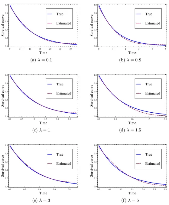
Clearly both bias and MSE are small and as the sample size n increases they decrease, as one would expect and the empirical coverage probabilities are found fairly large, closer to one. Also for each set of parameter values and with sample size 750 we shall find out a cubic polynomial estimate of the form S0(t) = c0+
c1t + c2t2+ c3t3 with each of its coefficients being the average of corresponding coefficients obtained for all the iterations, for the baseline survival function and are compared in Figure 1, where continuous curve represents the true baseline survival function and dotted curve represents corresponding estimate. We see that both the estimated curve and actual curve are very close to each case.
4. Data Analysis
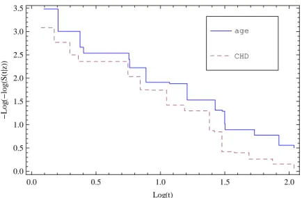
In this section we apply our model to a real life data set. We consider the data on survival times (in years) for 149 diabetic patients followed for 17 years studied by Lee et al. (1988) and the data is given in Lee and Wang (2003), pages 58-63. The original data consists of 8 potential prognostic variables, but for illustrative purpose we take only two among them namely age denoted by z1 and coronary heart disease(CHD) denoted by z2 as the covariates with respective regression coefficients θ1 and θ2. Censoring is made by the method follows. A random cen-soring interval (U, V ), where U and V − U are independent exponential variates with means λ−11 = 20 and λ−12 = 12.5 is generated first. Then an individual from among 149 patients is selected at random and if lifetime of the patient happens to fall in the generated censoring interval, that lifetime is assumed to have middle censored and that interval is considered as the corresponding observation. Other-wise the lifetime is maintained. This process is repeated until around 25% of the observations are censored. The data resulted consists of 36 censored observations. We apply the model given in Section 2 and find that the estimate of the baseline survival function is ˆS0(t) = 7.886× 10⁻⁷t3− 0.002272 t2− 0.22181 t + 0.880574 and the estimates of the regression coefficients are obtained to be ˆθ1 = 0.004418 and ˆθ2= 0.1096. i.e., the covariates have a positive effect on the lifetime. To test the significance of the covariate effect we consider the null hypothesis H0: θ = 0, where θ = (θ1, θ2) and 0 is null vector of same order, and we use the likelihood ra-tio test described in Remark 2. The P-value of 0.0382 indicates that the covariate effects are significant. To check the validity of proportional hazards assumption, we shall plot−log (−log (S(t|z))) against log t for the two covariates separately and the plots are given in Figure 2. We find that the two step functions are parallel and thus the proportionality assumption is justified.
0 5 10 15 20 25 30 0.0 0.2 0.4 0.6 0.8 1.0 Time Survival curve Estimated True 0 1 2 3 4 5 0.0 0.2 0.4 0.6 0.8 1.0 Time Survival curve Estimated True (a) λ = 0.1 (b) λ = 0.8 0.0 0.5 1.0 1.5 2.0 2.5 0.0 0.2 0.4 0.6 0.8 1.0 Time Survival curve Estimated True 0.0 0.5 1.0 1.5 2.0 0.0 0.2 0.4 0.6 0.8 1.0 Time Survival curve Estimated True (c) λ = 1 (d) λ = 1.5 0.0 0.2 0.4 0.6 0.8 0.0 0.2 0.4 0.6 0.8 1.0 Time Survival curve Estimated True 0.0 0.1 0.2 0.3 0.4 0.5 0.6 0.0 0.2 0.4 0.6 0.8 1.0 Time Survival curve Estimated True (e) λ = 3 (f) λ = 5
0.0 0.5 1.0 1.5 2.0 0.0 0.5 1.0 1.5 2.0 2.5 3.0 3.5 LogHtL -Log H-log HS Ht Èz LL CHD age
5. Conclusion
The present study discussed the semi-parametric regression problem for the anal-ysis of middle censored data. A maximization procedure for finding the NPMLE is developed and its consistency established. The model is applied to a real data set. Simulation studies show that the inference procedure is efficient. Although we have considered a cubic curve for approximating S0(t) in our example, the degree and nature of the curve, of course, depends on the data set and the censoring distribution. More studies in this direction will be carried out in a separate work. Asymptotic normality of ˆθ and weak convergence of ˆS0(t) do not appear to be easy to establish, although one can perhaps extend the ideas used in Huang and Wellner (1995).
Acknowledgements
We thank the editor and referee for their constructive comments on the manuscript.
References
A. Abuzaid, M. Abu El-Qumsan, A. El-Habil (2015). On the robustness of
right and middle censoring schemes in parametric survival models.
Communi-cations in Statistics-Simulation and Computation, , no. To appear.
N. Davarzani, A. Parsian (2011). Statistical inference for discrete
middle-censored data. Journal of Statistical Planning and Inference, 141, no. 4, pp.
1455–1462.
C. R. David (1972). Regression models and life tables (with discussion). Journal of the Royal Statistical Society, 34, pp. 187–220.
A. P. Dempster, N. M. Laird, D. B. Rubin (1977). Maximum likelihood from
incomplete data via the em algorithm. Journal of the royal statistical society.
Series B (methodological), pp. 1–38.
B. Efron (1967). The two sample problem with censored data. In Proceedings of
the fifth Berkeley symposium on mathematical statistics and probability. vol. 4,
pp. 831–853.
J. Huang, J. A. Wellner (1995). Efficient estimation for the proportional
hazards model with” case 2” interval censoring. Technical Report No. 290, Department of Statistics, University of Washington, Seattle, USA.
S. K. Iyer, S. R. Jammalamadaka, D. Kundu (2008). Analysis of
middle-censored data with exponential lifetime distributions. Journal of Statistical
Plan-ning and Inference, 138, no. 11, pp. 3550–3560.
S. R. Jammalamadaka, S. K. Iyer (2004). Approximate self consistency for
middle-censored data. Journal of statistical planning and inference, 124, no. 1,
S. R. Jammalamadaka, E. Leong (2015). Analysis of discrete lifetime data
under middle-censoring and in the presence of covariates. Journal of Applied
Statistics, 42, no. 4, pp. 905–913.
S. R. Jammalamadaka, V. Mangalam (2003). Nonparametric estimation for
middle-censored data. Journal of nonparametric statistics, 15, no. 2, pp. 253–
265.
S. R. Jammalamadaka, V. Mangalam (2009). A general censoring scheme for
circular data. Statistical Methodology, 6, no. 3, pp. 280–289.
J. D. Kalbfleisch, R. L. Prentice (2011). The statistical analysis of failure
time data, vol. 360. John Wiley & Sons.
J. P. Klein, M. L. Moeschberger (2005). Survival analysis: techniques for
censored and truncated data. Springer Science & Business Media.
J. F. Lawless (2011). Statistical models and methods for lifetime data, vol. 362. John Wiley & Sons.
E. T. Lee, J. Wang (2003). Statistical methods for survival data analysis, vol. 476. John Wiley & Sons.
E. T. Lee, M. A. Yeh, J. L. Cleves, D. Shafer (1988). Vascular complications
in noninsulin dependent diabetic oklahoma indians. Diabetes, 37,(Suppl. 1).
V. Mangalam, G. M. Nair, Y. Zhao (2008). On computation of npmle for
middle-censored data. Statistics & Probability Letters, 78, no. 12, pp. 1452–
1458.
P. G. Sankaran, S. Prasad (2014). Weibull regression model for analysis of
middle-censored lifetime data. Journal of Statistics and Management Systems,
17, no. 5-6, pp. 433–443.
P.-s. Shen (2010). An inverse-probability-weighted approach to the estimation of
distribution function with middle-censored data. Journal of Statistical Planning
and Inference, 140, no. 7, pp. 1844–1851.
P.-s. Shen (2011). The nonparametric maximum likelihood estimator for
middle-censored data. Journal of Statistical Planning and Inference, 141, no. 7, pp.
2494–2499.
J. Sun (2006). The statistical analysis of interval-censored failure time data. Springer Science & Business Media.
T. Tarpey, B. Flury (1996). Self-consistency: a fundamental concept in
statis-tics. Statistical Science, pp. 229–243.
W.-Y. Tsai, J. Crowley (1985). A large sample study of generalized maximum
likelihood estimators from incomplete data via self-consistency. The Annals of
B. W. Turnbull (1976). The empirical distribution function with arbitrarily
grouped, censored and truncated data. Journal of the Royal Statistical Society.
Series B (Methodological), pp. 290–295.
Summary
Middle censoring introduced by Jammalamadaka and Mangalam (2003), refers to data arising in situations where the exact lifetime becomes unobservable if it falls within a random censoring interval, otherwise it is observable. In the present paper we propose a semi-parametric regression model for such lifetime data, arising from an unknown population and subject to middle censoring. We provide an algorithm to find the non-parametric maximum likelihood estimator (NPMLE) for regression parameters and the survival function. The consistency of the estimators are established. We report simula-tion studies to assess the finite sample properties of the estimators. We then analyze a real life data on survival times for diabetic patients studied by Lee et al. (1988).