Stochastic Local Search for SMT: a Preliminary Report

(1)

UNIVERSITY

OF TRENTO

DIPARTIMENTO DI INGEGNERIA E SCIENZA DELL’INFORMAZIONE

38050 Povo – Trento (Italy), Via Sommarive 14

http://www.disi.unitn.it

STOCHASTIC LOCAL SEARCH FOR SMT: A PRELIMINARY

REPORT

Alberto Griggio, Roberto Sebastiani and Silvia Tomasi

May 2009

(2)

(3)

Stochastic Local Search for SMT: a Preliminary Report

(extended abstract)

Alberto Griggio, Roberto Sebastiani, and Silvia Tomasi DISI, Universit`a di Trento, Italy.

1 Introduction

A popular approach to SMT is based on the integration of a DPLL SAT solver and of a decision procedure able to handle sets of atomic constraints in the underlying theory T (T -solver). In pure SAT, however, stochas-tic local-search (SLS) [5] procedures sometimes outperform DPLL on sat-isfiable instances, in particular when dealing with unstructured problems. Therefore, it is a natural research question to wonder whether SLS can be exploited successfully also inside SMT tools.

The purpose of this paper is to start investigating this issue. First, we present an algorithm integrating a Boolean SLS solver (based on the WalkSAT paradigm) with a T -solver, resulting in a basic SLS-based SMT solver. Second, we introduce a group of techniques aimed at improving the synergy between the Boolean and the T -specific component, and discuss the differences between the integration of T -solvers with a DPLL-based and a SLS-based SAT solver. Finally, we perform a preliminary experimental evaluation of our implementation (based on the integration of the UBCSAT [10] SLS platform with the LA(Q)-solver of MathSAT [1]) by comparing it against MathSAT, a state-of-the-art DPLL-based SMT solver, on both structured industrial problems coming from the SMT-LIB and randomly-generated unstructured problems.

From this preliminary analysis we have that the performance of the SLS-based tool (i) is far from that of the DPLL-SLS-based one on SMT-LIB problems and (ii) is comparable on random problems.

2 Background

2.1 Stochastic Local Search for SAT

Local search (LS) algorithms [5, 4] are widely used for solving hard

combi-natorial search problems. The idea behind LS is to inspect the search space of a given problem instance starting at some position and then iteratively moving from the current position to a neighboring one where each move is

(4)

determined by a decision based on information about the local neighbor-hood. LS algorithms making use of randomized choices during the search process are called Stochastic Local search (SLS) algorithms. SLS algorithms have been successfully applied to the solution of many N P-complete decision problems, including SAT. Notice, however, that SLS algorithms typically do not guarantee that eventually an existing solution is found, so that they cannot verify the unsatisfiability of a problem.

SLS algorithms for SAT typically work with a CNF input formula (namely

ϕ) and share a common high-level schema: (i) they initialize the search by

generating an initial truth assignment (typically at random); (ii) they itera-tively select one variable and flip it within the current truth assignment. The search terminates when the current truth assignment satisfies the formula ϕ or after max tries sequences of max flips variable flips without finding a model for ϕ. The main difference in SLS SAT algorithms is typically given by the different strategies applied to select the variable to be flipped.

2.2 WalkSAT Algorithms

WalkSAT is a popular family of SLS-based SAT algorithms [5, 4]. The schema of such algorithms is shown in Algorithm 1. Initially, a complete truth assignment µ for the variables of the input problem ϕ is selected by InitialTruthAssignment according to some heuristic criterion (e.g., uniformly at random). If this assignment satisfies the formula, the algorithm terminates. Otherwise, a variable is selected and flipped in µ using a two-stage process. In the first two-stage, a currently-unsatisfied clause c is selected by ChooseUnsatisfiedClause according to some heuristic criterion (e.g., uniformly at random). In the second stage, one of the variables occurring in the selected clause c is flipped by NextTruthAssignment according to some mixed greedy/random heuristic criterion, so that to generate another truth assignment. The procedure is repeated until either a solution is found, or the limit of number of tries is reached.

Over the last ten years, several variants of the basic WalkSAT algorithm have been proposed [8, 6, 9], which differ mainly for the different heuristics used for the functions described above —in particular on the degree of greed-iness and randomness and in the criteria used for selecting the variable to flip in c within NextTruthAssignment. Currently, the best performing WalkSAT-based algorithm for SAT seems to be Adaptive Novelty+ _{[9]. For}

further details, we refer the reader to [5].

3 Stochastic Local Search for SMT

We start from a simple observation: from the perspective of a SAT solver, an SMT problem instance ϕ can be seen as the problem of solving a

(5)

Algorithm 1 WalkSAT (ϕ)

Require: CNF formula ϕ, max tries, max flips

1: for i = 1 to max tries do

2: µ ← InitialTruthAssignment(ϕ)

3: for j = 1 to max flips do

4: if (µ |= ϕ) then 5: return sat 6: else 7: c ← ChooseUnsatisfiedClause(ϕ) 8: µ ← NextTruthAssignment(ϕ, c) 9: end if 10: end for 11: end for 12: return unknown

abstraction of ϕ and the “invisible” part τp _{is (the Boolean abstraction of)}

the set of the T -lemmas providing the obligations induced by the theory T on the atoms of ϕ. (We use the superscriptp _{to denote the Boolean abstraction}

of a T -formula.) To this extent, a traditional “lazy” SMT solver can be seen as a DPLL solver which knows ϕp _{but not τ}p_{: whenever a model µ}p

for ϕp _{is found, it is passed to a T -solver which knows τ}p _{and hence checks}

if µp _{falsifies τ}p_{: if this is the case, it returns one clause c}p _{in τ}p _{which is}

falsified by µp_{, which is then used by DPLL to drive the future search and}

is optionally added to ϕp_.

The above observation inspired to us a procedure integrating a T -solver into a SLS algorithm of the WalkSAT family (WalkSMT hereafter).

3.1 A basic WalkSMT procedure

A high-level description of the pseudo-code of WalkSMT is shown in Algo-rithm 2. (We present first a basic version WalkSMT, in which we tem-porarily ignore steps 1-3 and 12-13, which we will describe in §3.2, to-gether with other enhancements.) WalkSMT receives in input a SMT(T ) CNF formula and applies a WalkSAT scheme to its Boolean abstraction

ϕp. InitialTruthAssignment, ChooseUnsatisfiedClause and Next-TruthAssignment are the functions described in §2.2. (Notice that their underlying heuristic vary with the different variants of WalkSAT adopted.) Ignoring steps 1-3 and 12-13, the only significant difference wrt. Algo-rithm 1 is in steps 7-14. Whenever a total model µp _{is found s.t. µ}p _{|= ϕ}p_,

it is passed to T -solver. If (the set of T -literals corresponding to) µp _{is T}

-satisfiable (i.e., µp |= ϕp∧τp) the procedures ends returning sat. Otherwise,

T -solver returns conflict and a T -lemma cp_{. Notice that this corresponds}

(6)

Algorithm 2 WalkSMT (ϕ)

Require: SMT(T ) CNF formula ϕ, max tries, max flips

1: if (T -preprocess (ϕ) == conflict) then

2: return unsat

3: end if

4: for i = 1 to max tries do

5: µp _{← InitialTruthAssignment (ϕ}p₎

6: for j = 1 to max flips do 7: if (µp |= ϕp) then

8: hstatus, cp_{i ← T -solver(ϕ}p_{, µ}p₎

9: if (status == sat) then

10: return sat 11: end if 12: cp ← Unit-Simplification(ϕp, cp) 13: ϕp ← ϕp∧ cp 14: µp_{← NextTruthAssignment (ϕ}p_{, c}p₎ 15: else 16: cp ← ChooseUnsatisfiedClause (ϕp) 17: µp_{← NextTruthAssignment (ϕ}p_{, c}p₎ 18: end if 19: end for 20: end for 21: return unknown

ϕp_{∧ τ}p _{which are falsified by µ}p_{. Thus, c}p _{is used by}

NextTruthAssign-ment as “selected” unsatisfied clause to drive the flipping of the variable. To this extent, T -solver plays the role of ChooseUnsatisfiedClause on

ϕp_{∧ τ}p _{when no unsatisfied clause is found in ϕ}p_.

3.2 Enhancements to the basic WalkSMT procedure

The WalkSMT algorithm described above is very simplistic, and can be optimized in several ways. In this section, we briefly describe some of the most significant optimizations that we have investigated.

Preprocessing. (Steps 1-3.) Before entering the main WalkSMT routine, we apply a preprocessing step to the input formula ϕ in order to make it simpler to solve. First, we perform a step of unit propagation, by substitut-ing each literal occurrsubstitut-ing as a unit clause in ϕ with true, repeatsubstitut-ing this step until a fixpoint is reached, and finally by re-adding to ϕ the conjunc-tion of all non-proposiconjunc-tional unit literals eliminated. (If during this process one of the clauses of ϕ becomes empty, the algorithm can exit returning unsat.) Second, we apply static learning [7], which augments the input

(7)

for-mula with short T -lemmas generated without invoking the T -solver, having the purpose of detecting a priori in a fast manner obviously T -inconsistent assignments to T -atoms.

Learning. (Step 13.) The second important optimization is that of learning the T -lemmas generated by the T -solver, as is done in DPLL-based SMT solvers, so that to avoid finding the same T -conflict (which might be quite expensive) multiple times.

Unit simplification. (Step 12.) Before learning a T -lemma, we remove from it (setting them to true) all the literals which occur as unit clauses in the (preprocessed) input problem.

Filtering the assignments given to T -solvers. In order to reduce the work that T -solvers have to do, we apply some standard filtering techniques to the current truth assignment before invoking the T -solver, such as pure

literal filtering and ghost literal filtering (see [7]).

Multiple learning. Unlike with DPLL-based SMT solvers, which typically use some form of early pruning to check partial truth assignments for T -consistency, in an SLS-based approach T -solvers operate always on complete truth assignments. In this setting, a truth assignment may be T -inconsistent for several different reasons, often independent from each another. This is the idea at the basis of our multiple learning technique, which allows for learning more than one T -lemma for every T -inconsistent assignment. In particular, when we find a conflict set η the (unit simplified) T -lemma ¬η is used to compute a subassignment µ0 _{s.t. µ}0 _{⊂ µ, on which the T -solver is}

invoked again to find a new conflict set. The subassignment µ0 _{is computed}

by dividing the current (unit simplified) T -lemma ¬η in f parts (where f is a parameter) and removing the variables occurred in the first part of it from

µ. This process is repeated until no conflict set is found. We then learn all

the T -lemmas generated during the process.

3.3 Efficient T -solvers for local search

In DPLL-based SMT solvers, the interaction with T -solvers is stack-based: the truth assignment µ is incrementally extended when performing unit propagation, T -propagation, and when picking an unassigned literal for branching, and it is partly undone upon backtracking, when the most-recently-assigned literals are removed from it. Consequently, T -solvers de-signed for interaction with DPLL are typically optimized for such stack-based invocation. In particular, they typically incremental (when they have to check the consistency of a truth assignment µ0 that is an extension of a previously-checked µ, they don’t need to restart the computation from scratch) and backtrackable (when backtracking occurs, the most-recently-assigned literals that need to be unmost-recently-assigned can be efficiently removed, and the internal state can be efficiently restored to a previous configuration) [7].

(8)

In local search, truth assignments are not updated in a stack-based man-ner. Rather, a new assignment µ0 _{is obtained from the previous one µ by}

flipping an arbitrary literal (according to some heuristics). In this setting, the conventional backtrackability feature of T -solvers is of little use, since there is no notion of most-recently-assigned literals to remove. Instead, it would be very desirable to be able to remove an arbitrary literal from a

T -solver without the need of resetting its internal state. Such requirement

might seem unrealistic, or at least difficult to fulfill. However, we are aware of at least two state-of-the-art T -solvers that have this capability: the solver for DL of [2] and the solver for LA(Q) of [3], which are therefore natural candidates for integration with a local-search-based SAT solver.

4 Preliminary Experimental Evaluation

We have implemented the SLS-based SMT procedure described above in our WalkSMT solver. WalkSMT was written in C++ by integrating the UBCSAT [10] SLS-based SAT solver (using the Adaptive Novelty+ _variant

of the WalkSAT family) with the LA(Q)-solver of [3] that is implemented within MathSAT 4 [1]. In this section, we evaluate the performance of WalkSMT by comparing it against a state-of-the-art SMT solver based on DPLL. We consider three versions of WalkSMT:

• Basic-WalkSMT, which does not include improvement techniques;

• Learning-WalkSMT, combining Basic-WalkSMT with preprocess-ing, unit simplification and simple learning optimizations of §3.2;

• Best-WalkSMT, which extends Learning-WalkSMT with the mul-tiple learning (with f = 1), pure-literal filtering and ghost-literal fil-tering optimizations of §3.2.

In order to minimize the performance differences due to the implementa-tion, we adopted MathSAT as DPLL-based SMT solver for the comparison, since, as mentioned above, WalkSMT uses the same LA(Q)-solver as Math-SAT. Moreover, in order to better isolate the different factors that influence the performance of a DPLL-based SMT solver, we ran MathSAT in two dif-ferent configurations: a “full” one with all the optimizations enabled, and a “restricted” one in which we disabled two important optimizations that are impossible to apply in an SLS-based algorithm, namely early pruning and

T -propagation.

We performed our comparison over two distinct sets of instances, which are described in the next two sections: the first consists of a subset of the formulas in the SMT-LIB (www.smtlib.org), whereas the second is composed of randomly-generated problems. All tests were executed on 2.66 GHz Xeon machines running Linux, using a timeout of 600 seconds.

(9)

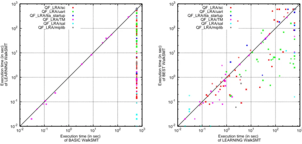
10-2 10-1 100 101 102 103 10-2 ₁₀-1 ₁₀0 ₁₀1 ₁₀2 ₁₀3

Execution time (in sec) _{of LEARNING WalkSMT}

Execution time (in sec) of BASIC WalkSMT QF_LRA/sc QF_LRA/uart QF_LRA/tta_startup QF_LRA/TM QF_LRA/sal QF_LRA/miplib 10-2 10-1 100 101 102 103 10-2 ₁₀-1 ₁₀0 ₁₀1 ₁₀2 ₁₀3

Execution time (in sec) of BEST WalkSMT

Execution time (in sec) of LEARNING WalkSMT QF_LRA/sc QF_LRA/uart QF_LRA/tta_startup QF_LRA/TM QF_LRA/sal QF_LRA/miplib

Figure 1: Comparison of different configurations of WalkSMT on SMT-LIB instances.

4.1 SMT-LIB Instances

In the first part of our experiments, we compare WalkSMT against Math-SAT on a subset of the satisfiable LA(Q)-formulas (QF LRA) in the SMT-LIB. These instances are classified as “industrial”, and they come from the encoding of different real-world problems in formal verification, planning and optimization. The results of the experiments are reported in Figures 1 and 2: Figure 1 shows the effects of the different optimizations we intro-duced for the WalkSMT algorithm, whereas Figure 2 compares the best configuration of WalkSMT with the two configurations of MathSAT.

The results clearly show that:

1. Learning the discovered T -lemmas is crucial for performance. Without it, WalkSMT times out on almost all instances;

2. The optimizations described in §3.2 lead to very significant improve-ments, sometimes by orders of magnitude;

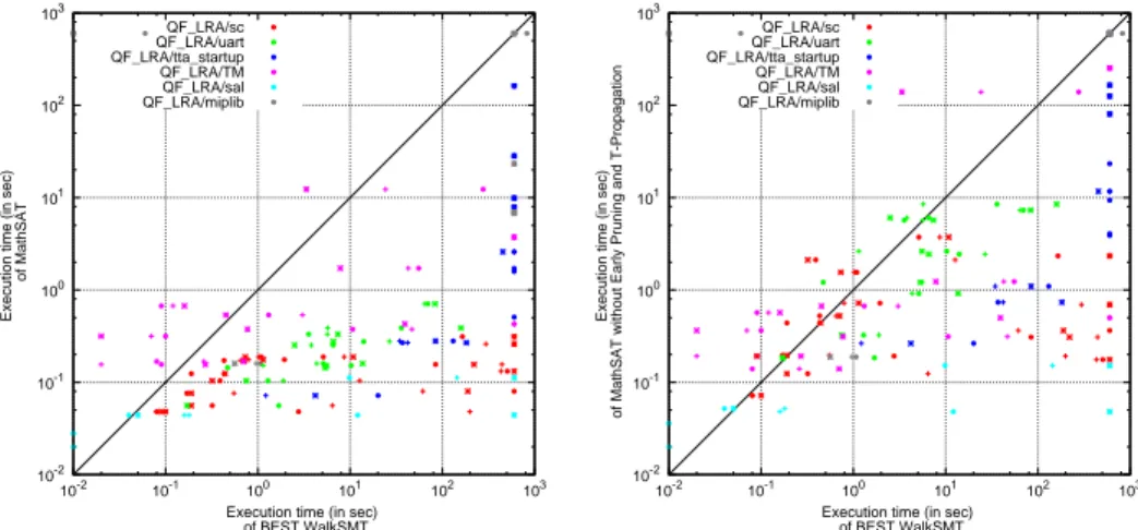
3. Despite the improvements, the gap between WalkSMT and Math-SAT is still huge. This is in part explained by the use of early pruning and T -propagation within MathSAT, as Figure 2 shows. Such opti-mizations are not possible to implement within WalkSMT, since in local-search-based algorithms there is no concept of partial truth as-signment, and the T -solver always operates on complete assignments. However, even with early pruning and T -propagation turned off (right plot of Figure 2), the performance of MathSAT is still much better than that of WalkSMT. This is not surprising, as it reflects the well-known fact that even for pure propositional problems DPLL-based

(10)

10-2 10-1 100 101 102 103 10-2 ₁₀-1 ₁₀0 ₁₀1 ₁₀2 ₁₀3

Execution time (in sec)

of MathSAT

Execution time (in sec) of BEST WalkSMT QF_LRA/sc QF_LRA/uart QF_LRA/tta_startup QF_LRA/TM QF_LRA/sal QF_LRA/miplib 10-2 10-1 100 101 102 103 10-2 ₁₀-1 ₁₀0 ₁₀1 ₁₀2 ₁₀3

Execution time (in sec)

of MathSAT without Early Pruning and T-Propagation

Execution time (in sec) of BEST WalkSMT QF_LRA/sc QF_LRA/uart QF_LRA/tta_startup QF_LRA/TM QF_LRA/sal QF_LRA/miplib

Figure 2: Comparison of Best-WalkSMT with the two configurations of MathSAT on SMT-LIB instances.

SAT solvers outperform SLS-based ones on industrial, structured in-stances, where the power of Boolean Constraint Propagation can be fully exploited.

4.2 Random Instances

In the second part of our experiments, we compare WalkSMT against MathSAT on randomly-generated, unstructured LA(Q)-formulas. The set consists of 3-CNF instances generated in terms of the tuple of parameters

hm, n, ai where m is the number of clauses, n is the number of T -variables

and a is the number of distinct T -atoms occurring in the formula, where each T -atom is a polynomial P_ic_ix_i ≤ c₀ with exactly four variables with non-zero coefficient.

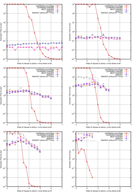
Figure 3 shows the run times of several versions of WalkSMT and MathSAT on the generated formulas, for n = 20. Each graph shows curves for Basic-WalkSMT, Learning-WalkSMT, Best-WalkSMT, MathSAT and MathSAT without early pruning and T -propagation on a group of in-stances with a fixed number a of T -atoms, for a = 30, 40, 50, 60, 70, 80. The plots represent the execution time versus the ratio r = m/a of clauses/T -atoms. Each point in the graphs corresponds to the median run-time of each algorithm on 20 different instances of the same size. (For WalkSMT, each value is itself a median value of 3 to 7 druns with different seeds.) The plots show also the satisfiability percentage of each group of instances, defined as the ratio between the satisfiable instances generated and the total number of instances generated, for each value of r. For example, in the plot located in the first column of the last row of Figure 3 the percentage 0.001% for r = 5 means that we had to generate 337631 formulas (using MathSAT with a timeout of 600 seconds) in order to obtain 20 satisfiable instances.

(11)

10-3 10-2 10-1 100 101 102 103 2 3 4 5 6 7

Execution Time (in sec)

Ratio of clauses to atoms, r=m/a where a=30 satisfiability percentage

LEARNING WalkSMT BEST WalkSMT MathSAT MathSAT without EP T-Prop

10-3 10-2 10-1 100 101 102 103 2 3 4 5 6 7

Figure 3: Comparison of different configurations of WalkSMT and Math-SAT on randomly-generated instances with 20 theory variables and atoms

(12)

The results show that there is a very small difference between the per-formance of Learning-WalkSMT and Best-WalkSMT. Moreover, unlike with SMT-LIB formulas, on randomly-generated instances the performance of Learning-WalkSMT, Best-WalkSMT and MathSAT is almost identi-cal. Moreover, as with SMT-LIB instances, early pruning and T -propagation play a very important role in the performance of MathSAT, especially on the hardest formulas (last three plots).

References

[1] R. Bruttomesso, A. Cimatti, A. Franz´en, A. Griggio, and R. Sebastiani. The MathSAT 4 SMT Solver. In Proc. of CAV, volume 5123 of LNCS, pages 299–303. Springer, 2008.

[2] S. Cotton and O. Maler. Fast and Flexible Difference Constraint Prop-agation for DPLL(T). In SAT, volume 4121 of LNCS. Springer, 2006.

[3] B. Dutertre and L. de Moura. A Fast Linear-Arithmetic Solver for DPLL(T). In CAV, volume 4144 of LNCS, 2006.

[4] H. H. Hoos and T. Stutzle. Local Search Algorithms for SAT: An Empirical Evaluation. Journal of Automated Reasoning, 24(4):421–481, 2000.

[5] H. H. Hoos and T. Stutzle. Stochastic Local Search Foundation And

Application. Morgan Kaufmann, 2005.

[6] S. Minton, M. D. Johnston, A. B. Philips, and P. Laird. Minimizing Conflicts: A Heuristic Repair Method for Constraint-Satisfaction and Scheduling Problems. Artificial Intelligence, 58(1):161–205, 1992.

[7] R. Sebastiani. Lazy Satisfiability Modulo Theories. Journal on

Satisfi-ability, Boolean Modeling and Computation, JSAT, Volume 3, 2007.

[8] B. Selman, H. A. Kautz, and B. Cohen. Noise strategies for improving local search. In Proceedings of the Twelfth National Conference on

Artificial Intelligence, pages 337 – 343. MIT Press, 1994.

[9] D. Tompkins and H. Hoos. Novelty+ and Adaptive Novelty+. SAT

2004 Competition Booklet, 2004.

[10] D. Tompkins and H. Hoos. UBCSAT: An Implementation and Exper-imentation Environment for SLS Algorithms for SAT and MAX-SAT. In SAT, volume 3542 of LNCS. Springer, 2004.