UNIVERSITY
OF TRENTO
DIPARTIMENTO DI INGEGNERIA E SCIENZA DELL’INFORMAZIONE
38050 Povo – Trento (Italy), Via Sommarive 14 http://www.disi.unitn.it
ANALYSIS OF TCP/MAC INTERACTIONS USING THE GAME THEORY
Christian Facchini and Fabrizio Granelli
May 2008
Technical Report # DISI-08-025
A
NALYSIS OF
TCP/MAC
I
NTERACTIONS
U
SING THE
G
AME
T
HEORY
Christian Facchini, Fabrizio Granelli
Abstract
ISO/OSI and TCP/IP protocol stacks provide networks and devices interoperability by exploiting the principle of layering, where every layer is characterized by specific functionalities and is allowed to interact only with adjacent layers by means of standardized interfaces. However, while such principle provides freedom in implementation of the protocols at different layers, it limits the control on the interaction among protocols at different layers. In this framework, it is necessary to develop efficient model to capture the interaction of protocols with a single communication device in order to underline such forms of “indirect” interaction – which may lead to unforeseen performance degradations. The proposed work aims at proposing the usage of the game theory for capturing the interactions within the protocol stack of a single node, with the goal of allowing to determine the “steady state” or the operating point of the system in a given scenario (TCP over IEEE 802.11).
1. Introduction
ISO/OSI and TCP/IP protocol stacks were developed with the goal of enabling interoperability and foster development and diffusion of networks and network devices. The basic principle of such standardization activity is “layering”, i.e. to associate specific communication functionalities to different layers and allowing interaction between adjacent layers only in a server/client manner.
The main layering concepts are the following:
- Each layer performs a subset of the required communication functions - Each layer relies on the next lower layer to perform more primitive functions - Each layer provides services to the next higher layer
- Changes in one layer should not require changes in other layers.
A protocol at a given layer is implemented by a (software, firmware, or hardware) entity, which communicates with other entities (on other networked systems) implementing the same protocol by Protocol Data Units (PDUs). A PDU is built by payload (data addressed or generated by an entity at a higher adjacent layer) and header (which contains protocol information). PDU format as well as service definition is specified by the protocol at a given level of the stack.
The main advantage deriving from the layering paradigm is the modularity in protocol design, which enables interoperability and improved design of communication protocols. Moreover, a protocol within a given layer is described in terms of functionalities it offers, while implementation details and internal parameters are hidden to the remainder layers (the so-called “information-hiding” property).
As a consequence of the layering structure in today’s communication systems, all protocols at all layers concur to defining the overall performance - while being characterized by different and sometimes contrasting goals. This gives rise to cross-dependency and introduces complex interactions among protocols at different (even not adjacent) layers.
Given the complexity of such interactions, widely used models for evaluation of communication performance focus on a single layer only. Therefore, no formal characterization of the inter-layer (or cross-layer) interaction among different levels of the protocol stack is available yet, with the exception of [1], where the impact of different layers is studied in order to optimize service delivery in mobile ad-hoc networks, and [2], where the authors introduced a metamodeling approach to study cross-layer scheduling in wireless local area networks.
As it is correctly pointed out in [3], there is a need for a “holistic” approach to understanding and exploiting cross-layer interactions. The subject of systematic study of cross-layering from a “system theoretic” point of view and the closest available to a holistic view, is found in the work of Law and Doyle, for example [4]. The authors follow a top-down approach to set “holistic” objectives as opposed to the wide-spread “bottom up” and “ad hoc” identification and usage of cross-layer formulations on a case by case empirical basis.
A clear need is thus emerging for defining a framework able to capture inter-layer interactions in order to augment the possibility of studying communication performance. As inter-layer interactions are triggered by direct or indirect PDU exchange or service requests, the authors believe that more emphasis should be given to interaction rather that single-layer modeling. In this scenario, an appropriate framework to be considered is represented by the game theory which fits the requirements of addressing interactions between multiple players with different goals and strategies.
The paper is aimed at defining a suitable model to characterize inter-layer interactions by using the game theory and validating it in a “TCP over WLAN” scenario. The following sections just outline the main features of the proposed approach, while some mathematical details are left outside of the presentation for sake of clarity.
2. Game theory principles
Game theory deals with the analysis and the solution of conflicting situations present in a group of decision-makers, technically referred to as “players”. Players' decisions are driven by their own willingness to achieve a particular target, that is, they are carefully chosen in order to get the maximum possible reward (also known as the “payoff”). Furthermore, since it is likely these decisions affect each other's reward, every player has to take into account this interdependence and act accordingly.
These assumptions, commonly credited as “rationality assumption” and “strategic behavior”, form the basis of game theory.
Game theory was born and was initially applied in the economic field; though, its application spread virtually wherever there were conflicts to be studied, the area of communication networks being no exception. However, networks have been investigated by means of this theory only in recent times: as a matter of fact, the early studies of wired networks can be traced back to the end of the nineties; instead, wireless networks have been analyzed starting only few years ago [5].
What makes the application of game theory interesting is the capability to find the so-called “equilibria” of a game, which are, broadly speaking, particular system configurations that are optimal from every player's point of view. In other words, when the game reaches an equilibrium, players who try to change their actions inevitably end up with a smaller payoff. From another perspective, these peculiar configurations can also be interpreted as steady states of the system.
More important, games may have one or multiple equilibria or may even have no equilibrium whatsoever. Besides, not all the equilibria are identical with one another: different types of equilibrium are possible, depending on the game characteristics.
However, before formally analyzing what kinds of game exist, it is mandatory to take a step back and introduce some fundamental quantities.
Let us start by assuming that I is the set of players. Then each player i has an action set, denoted by Ai, defining what actually a player can do, i.e. the actions he can choose. The
ensemble of actions chosen by all the players is an element belonging to the spaceA xjIAj, is referred to as “action profile”, and represents a possible outcome of the game. Because of their rationality, players are able to list each outcome in order of preference: the role of payoffs is to respect these preferences. Formally, a payoff function is a function u:A→ , mapping all the action profiles to real values so that ui(x)ui(y) if the player i prefers the outcome x over the outcome y. Finally, a strategy for a player i specifies what action is to be taken at every given point of the game. Strategies can be “pure” or “mixed”, whether they are completely deterministic or not. Pure strategies are usually denoted with latin letters, like si, while mixed strategies are rather denoted with
greek letters, such as σi. Besides, just like for actions, it is possible to define a strategy
profile (although it is useful only when the action set and the strategy set are different, as, for instance, in dynamic games).
As for the games, there are static (or strategic) and dynamic ones. In static games players take an action once and for all, and simultaneously (or, seen the other way around, the order in which actions are taken is unimportant). More specifically, a static game is thoroughly defined by a set of players, a non-empty action set and a payoff function for each player, and is usually represented through the so-called strategic form (which is but a n-dimensional matrix, n being the cardinality of the set of players). In this type of games the equilibrium is called “Nash equilibrium”, in honor of John Nash, and is an action profile so that: I i A a a a u a a ui i i i i i i , ) , ( ) , (
where a-i is short for (a1,,ai1,ai1,,a|I|). As can be easily seen, in such a situation no
player can profit by unilaterally deviating his own behavior.
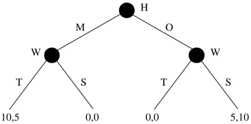
Dynamic games introduce the time consistency, in that actions are taken according to a specific chronological order. To effectively depict such games, generally a tree is used: in this representation, known as extensive representation, nodes indicate that some player has to take a decision, while the branches stemming from a node stand for the actions which can be actually taken. In general, not all the nodes get visited during the game, so it may happen that never visited paths contain some equilibria. As an example, let us think about a simple game, we call it “holiday game” (depicted in Figure 1): husband and wife are planning to go on holiday. He has to take care of the tickets and she, later, has to go and get the clothing. He may buy tickets to either the mountain or the ocean, while she has to choose between a trekking suit and a swimsuit. The husband prefers going to the mountain and the wife likes better go swimming rather than trekking; still, both of them prefer having their trekking suits when on the mountain and the swimsuits when in the ocean.
Figure 1. Extensive form of the “holiday game”.
Actions for him are simply M or O, whereas T or S are hers. As for the strategies, his strategy and action sets are the same; her strategy set, instead, contains four different elements, namely: TT, TS, ST, and SS. For instance, ST, means “to buy swimsuits in case he bought the tickets to the mountain and the trekking suits in case he bought the tickets to the ocean”. As a result, there are three Nash equilibria in this game when pure strategies are employed: M,TT M,TS and O,SS. Now, O,SS is not a proper solution: it's like saying she is going to get the swimsuits no matter what the husband chooses. This is called “empty threat”, as she is not really going to buy swimsuits if her husband brings home the tickets to the mountain (because she is rational and wants to maximize her payoff). That is why an equilibrium refinement is needed, in order to take into account the sequential structure of these games; particularly, the concept of “sub-game perfect equilibrium” is introduced. A sub-game is defined as a part of the tree starting not from any node in particular, and containing all the following nodes1.
An equilibrium is said to be sub-game perfect if it is a Nash equilibrium for each and every tree. Back to the example, the only game perfect equilibrium is M,TS: for the sub-game starting after the husband has chosen to go to the mountain, the Nash equilibrium is to take the trekking suits, while for the sub-game starting after the ocean has been chosen, is to take the swimsuits. The fact that the man buys the tickets to the mountain and that wife's strategy is TS, is a Nash equilibrium for that game.
Furthermore, dynamic games can be subdivided in games of complete and incomplete information. In games of complete information every player is aware of all the adversaries' moves, that is, everyone knows what action has been chosen, at any given point of the game, just like in the previously mentioned “holiday game”. On the contrary, in games of incomplete information players do know that a precise opponent has taken an action, yet they don't know which particular action has been taken. The “holiday game” can be easily turned into an incomplete information game: let us assume the husband goes buying the tickets but, once he comes back, doesn't keep her wife posted about the chosen location. Though she has no clue about her husband's choice, she is perfectly aware it's her turn to go shopping (as he has come back home).
As a side note, it should noted that it is pointless to talk about complete and incomplete information as far as static games are concerned: in such scenarios, moves are taken at the same time. Nevertheless, both static and dynamic games may be of perfect or imperfect information. A game is said to be of perfect information as long as all the players knows everything about the structure of the game (that is, other players, action sets, payoffs, …). Needless to say, if some aspects are unknown to at least one player, the game is an imperfect information one. Since the perfectness and the completeness of the
1
A proper and rigorous definition should also involve the case of games of incomplete information, still this falls behind the scope of this short introduction.
H W W 10,5 0,0 0,0 5,10 M O T S T S
information address two different kinds of knowledge, dynamic games can of any type: complete and perfect information (the first example presented), incomplete but perfect information (the second example), complete but imperfect (for instance, if the wife knows which location her husband has chosen but she doesn't know his preference), and incomplete and imperfect (when she doesn't know neither his choice, nor his preference). Static games of imperfect information are also known as Bayesian games, and are defined by a set of players, a non-empty action set and a payoff function for each player (just like static games of perfect information) and a set of “player beliefs”, describing every player's uncertainty about what is unknown. In these games, a special player, the Nature, moves first and determines each player's “type” (each type has its own characteristics): every player will know only his own type and no other one. Then the game follows its normal course, in that the players move simultaneously and get their payoff, with a minor difference: now strategies and actions are different, in fact, strategies are built upon actions and possible types. The equilibrium is no more known as Nash equilibrium, rather as “Bayesian Nash equilibrium”, although the underlying concept remains the same.
The same goes for dynamic games of imperfect information. These kinds of game are characterized by “Perfect Bayesian equilibria”, which are a refinement of the “Bayesian Nash equilibria” and take into account the possibility of empty threats.
On top of that, games can be played just once (stage game) or more than once (repeated games) or even be composed of different states. These ones, in particular, are based on the idea that the periods of a game can be summarized by a “state variable” [6] and are known as stochastic games (by the way, repeated games can be seen as a special case of stochastic games). Stochastic games are defined by a state variable, an action set for each player, a transition function, which expresses the probability of jumping across states, and the payoff functions, as usual. What is important, is that actions only depend on the current state, and payoff functions as well as the transition function depend on the current state and the current action chosen. As for strategies, “Markov strategies” can be defined as strategies that are only based on the current state of game and are independent of the whole game history [7]. A Markovian strategy profile resulting in a Nash equilibrium for every sub-game goes under the name “Markov Perfect equilibrium”.
Summarizing, equilibria not always exist. Some theorems come in handy for finding if, in a particular game, there are equilibria or not. Most notably is the Nash theorem, which states that every game having a finite players set and a finite and discrete strategy set, presents at least one Nash equilibrium.
Finally, a last clarification is needed: what has been presented is just a part of the game theory. In particular, all these games belong to the “cooperative” game theory, which identify players with single individuals. For the sake of completeness, the other part, that is, “non-cooperative” game theory uses players to symbolize groups of individuals [8].
3. The Proposed Approach
Our approach aims at using the game theory in order to model protocol entities in a host protocol stack. In particular, players represent specific layers, not necessarily adjacent with one another. It may be pointed out that non-adjacent layers do not have any relationship (as consecutive layers do, on the contrary), yet this is not correct. Although it is unquestionable that two non-consecutive layers have no direct relations, they experience sort of an indirect feedback (or feedforward), which is physically given by the immediately preceding (or following) layer, but it can be seen as if it were recursively generated from another layer following the PDU flows up and down the protocol stack.
Once players have been identified, actions and payoffs have to be specified. The action set is, as we have already discussed, what a player can actually do, so the best way to get
to know all a protocol's capabilities is to peer directly at the standard defining it. Nonetheless, the task of correctly determining actions by means of the standard is not a straightforward one at all. This happens because usually protocols are rather sophisticated and have to take care of many different aspects, therefore it is important to distinguish between actions that are useful in order to model the game and actions that are not. A similar thought also applies when looking for the right payoff function to use: this function mathematically translates the protocol's behavior, so it goes without saying how much care has to be taken when defining it.
Finally a proper kind of game has to be chosen. Whether to set up a static or a dynamic one, to decide to create one of perfect or imperfect information, etc., that all depends on the particular situation modeled. Anyway, it should not be forgotten that there is no such thing like “the one and only game”: different games may model the same scenario. Some games could faithfully represent certain aspects that others do not take into consideration at all (and vice versa, of course); or, some games may let to catch some particulars that other models give for granted, and so on.
We present here a simple scenario, aiming at illustrating the potentials of our approach. Let us consider an ad-hoc network, made up of two stations only. Each station is provided with a full TCP/IP stack, and uses TCP Tahoe as the transport layer protocol and IEEE MAC 802.11b as the MAC layer protocol. A station sends a continuous data flow, where the segment dimension is the same (and the biggest) for all the packets. The other station act as a receiver and acknowledges every incoming packet. The RTS/CTS mechanism is not employed, as its use is pointless, nor fragmentation is performed, because the channel is assumed ideal (so that no transmission errors are experienced).
There are two players, namely the TCP and the MAC entities on the sender station. The remote MAC entity is not represented, as it has no impact on the sender: since the communication is ideal it only acknowledges every incoming frame. As for the transport layer, we can neglect the remote TCP entity by simply assuming that the receiver's advertised window is always greater than the congestion window kept by sender (which is generally true, unless the receiver is experiencing technical difficulties). This way we can simplify the whole model and make the analysis simpler, too. However, it is worth noting, this doesn't mean it is not possible to model restrictions imposed by the receiver station, but only that we can decide whether to take them into account or not.
What TCP aims to do is made explicit by the relative RFC [9]: the target is to maximize the connection throughput, still trying not to run into congestion. The MAC's target is somehow similar, that is, to achieve the greatest throughput possible (at the data-link layer, naturally), and can be learnt from the IEEE 802.11 MAC/PHY specifications [10].
An outline of the action sets can be drawn by observing how players try to achieve their objectives. TCP increases the overall throughput by increasing its own congestion window, it only decreases it when timeout are experienced. This suggests that TCP's action space has to do with the congestion window size. The MAC player, on the other hand, blindly forwards on the medium what it is given from the above layers; this means that MAC actions: (i) depend on higher layers' actions, and (ii) deal with the number of frames delivered to the channel.
The game has to be such that the chronological order of the actions is maintained; in fact, the first mover should be the TCP entity, being the one that creates the packets, and only after, the MAC player takes these packets to form frames. For this purpose, a good model is represented by a dynamic game. Unfortunately, a single stage dynamic game cannot keep track of the evolution of the congestion window; a stochastic game can, though, by letting the state variable record the congestion window dimension. Then, the action spaces will change accordingly, that of TCP as a function of the state variable k, while that of MAC as a function of the TCP action set.
Being more precise, the player set comprises two players, that is: I={TCP,MAC}
While the action sets are as follows:
avoidance
collision
start
slow
}
0
,
,
1
,
{
}
0
,
,
1
2
,
2
{
k
k
k
k
a
k
k
a
A
th th th th k k TCP
) ( } 0 , , 1 , {k k k a k A TCP t t t MAC As for the payoff functions, they are defined this way:
MAC for TCP for ) , ( if ) , ( ) , ( and ) 0 , 0 ( ) 1 , 1 ( ) 0 , 1 ( ) 2 , 1 ( ) 1 , 1 ( ) 0 , ( ) 1 , ( ) , ( m R m m u n m R n n u R m m u u u n u n n u n n u n u n n u n n u
The game only misses its transition function, which tells how the congestion window evolves. TCP Tahoe increases its congestion window unless a timeout is experienced. The channel is ideal by hypothesis, so only collisions may have some effect on the communication. Anyway, this effect is negligible, in that the number of collisions is too low to cause a layer 4 timeout. On the other hand, if the MAC player sends less frames than how many packets he received, a timeout will be necessarily triggered. That said, the transition function can be expressed this way:
1
))
,
(
,
|
0
(
1
))
,
(
,
|
0
(
))
,
(
,
|
(
))
,
(
,
|
1
(
1 1 1 1n
m
n
a
k
k
k
k
q
p
n
n
a
k
k
k
q
p
n
n
a
k
k
k
k
q
p
n
n
a
k
k
k
k
k
q
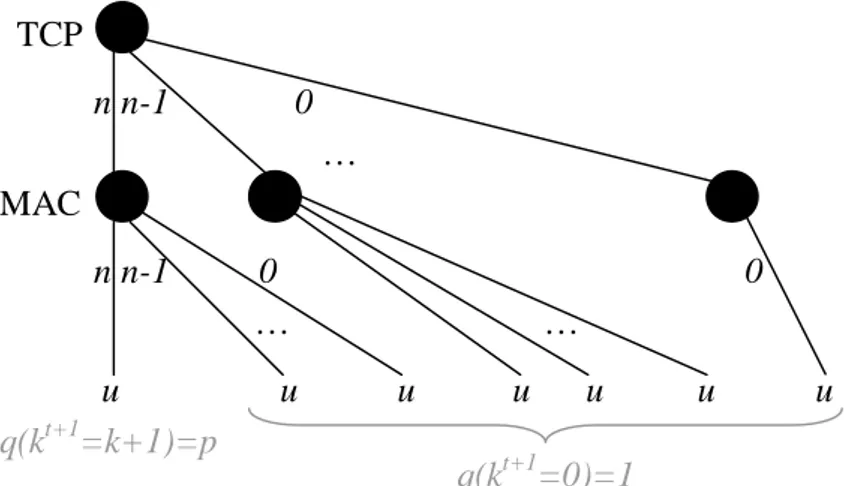
t M t t t t t t M t M t t M t tFigure 2. Tree representation of a generic game state k, where the congestion window size is n. u is nothing
but a placeholder for the actual utility.
The game starts with the smallest congestion window possible. Here, the TCP player is allowed to send only a segment, and that is what TCP will do, according to its payoff function. MAC will be given the segment and will decide to forward it to the channel. This is what happens in the game and thoroughly what happens in reality.
Moving a step further, it is important to stress what are the players' strategies, informally:
TCP thinks that, as up to n segments can be sent in this current stage, it is better to
send as many as possible of them (that is, n);
MAC thinks that, because if has received n segments in this current stage, it is better to
deliver them all.
The strategy profile st is then:
)
0
,
,
1
)}
(
sup{
)},
(
sup{
)};
(
(sup{
TCP t TCP t TCP t tk
A
k
A
k
A
s
Indeed, this is a “Markov strategy profile”, because strategies take into account only the current stage, and what is more, lead to a “Markov Perfect equilibrium”. In fact, no one can gain a bigger reward, at any given state of the game, by simply taking another action. As timeouts will not occur, the congestion window will continuously increase, ideally up to its maximum. Hence, it is possible to compute the throughput for a generic state, by having the number of correctly delivered bits divided by the time taken to accomplish the operation.
4. Results
The proposed model was validated by means of extending simulations using Network Simulator 2 (ns-2) environment. Simulations validate the model, as shown in Fig. 3, where as a results of absence of errors and collisions the TCP congestion window continuously increases. MAC … … … TCP n n-1 0 n n-1 0 0 q(kt+1=k+1)=p q(kt+1=0)=1 u u u u u u u
Figure 3. TCP congestion window evolution in the considered scenario.
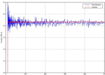
As a result, throughput computed following the proposed model is very close to that simulated, as it can be seen in Figure 4.
Figure 4. Comparison between throughput computer using the proposed approach and ns-2 simulations.
5. Conclusions
The use of game theory for modeling the behavior of protocol entities within a host protocol stack has a great potential. In this report, a sample scenario is presented to outline potential applicability of the idea to analyzed inter-later (or cross-layer) interactions. The same example could be extended to encompass more complex scenarios, for example including channel noise and multiple access.
Moreover, new players could be added to the model, such as a layer 3 player could be inserted in order to include routing, or to replace existing ones, such as other TCP versions other than Tahoe.
The final goal of the approach will be to investigate cross-layering architectures both as an analysis and synthesis tool, being able to capture and represent the effects of a protocol behaviour on others on the overall system performance.
References
[1] K.K. Vadde, V.R. Syrotiuk, “Factor Interaction on Service Delivery in Mobile Ad Hoc Networks,” IEEE Journal on Selected Areas In Communications (JSAC), Vol. 22, No.7, pp. 1335-1346, 2004. [2] J. Hui, M. Devetsikiotis, “Metamodeling of Wi-Fi Performance,” Proc. IEEE ICC 2006: Istanbul, Turkey, 2006.
[3] V. Kawada, P.R. Kumar, “A Cautionary Perspective on Cross-Layer Design,” IEEE Wireless Communications, Vol. 12, No.1, pp. 3-11, 2005.
[4] M. Chiang, S.H. Low, A.R. Calderbank, J.C. Doyle, “Layering as Optimization Decomposition: A Mathematical Theory of Network Architectures,” Proceedings of the IEEE, Vol. 95, No.1, pp. 255–312, 2007.
[5] V. Srivastava, J. Neel, A.B. Mackenzie, R. Menon, L.A. Dasilva, J.E. Hicks, J.H. Reed, and R.P. Gilles. Using game theory to analyze wireless ad hoc networks. Communications Surveys & Tutorials, IEEE, 7(4):46–56, 2005.
[6] D. Fudenberg, and J. Tirole. Game Theory. Mit Press, 1991.
[7] E. Rasmusen. Games and Information: An Introduction to Game Theory. Blackwell Publishing, 2006.
[8] M.J. Osborne, and A. Rubinstein. A Course in Game Theory. MIT Press, 1994.
[9] J. Postel. Transmission Control Protocol. RFC 793 (Standard), settembre 1981. Updated by RFC 3168.
[10] IEEE Working Group 802.11. Information technology- Telecommunications and information
exchange between systems- Local and metropolitan area networks- Specific requirements- Part 11: Wireless LAN Medium Access Control (MAC) and Physical Layer (PHY) Specifications. ANSI/IEEE Std 802.11, 1999 Edition (R2003), pp. i–513, 2003.