One "monetary giant" with many "fiscal dwarfs": The efficiency of macroeconomic stabilization policies in the European Monetary Union

UNIVERSITA

'

-

One "monetary giant" with many "fiscal dwarfs":

The efficiency of macroeconomic

stabilization policies in

the European Monetary Union

Roberto Tamborini

The Discussion Paper series provides a means for circulating preliminary research results by staff of or visitors to the Department. Its purpose is to stimulate discussion prior to the publication of papers.

Requests for copies of Discussion Papers and address changes should be sent to:

Prof. Andrea Leonardi Dipartimento di Economia Università degli Studi Via Inama 5

One "monetary giant" with many "fiscal

dwarfs": The efficiency of macroeconomic

stabilization policies in the European

Monetary Union

Roberto Tamborini

!!! "# !!!!

$ % & & ' (

13th World Congress, International Economic Association, Lisboa (Portugal), September 2002.

Abstract

One of the key problems in the design of a currency union is macroeconomic stabilization. Assuming that all policy-makers in the European Monetary Union are "disciplined" according to the rules set by the Maastricht Treaty and the Stability and Growth Pact, this paper addresses the question of whether member countries will effectively be sheltered against undesirable macroeconomic fluctuations. The analytical thrust of the paper is that having disciplined policy-makers does not exhaust the problem of policy design. Stabilization in the EMU may be pursued by means of centralized monetary policy as well as by means of national fiscal policies. Hence, the Tinbergen-Meade problem of efficient choice and assignment of stabilization instruments arises, a problem that has hitherto been disregarded. The main conclusion is that the now popular idea that the European Central Bank will cope with union-wide shocks while national governments will stabilize domestic shocks is not always the most efficient assignment choice, and it is inconsistent with the imposition of a fiscal deficit ceiling on member countries.

Keywords: European Monetary Union, macroeconomic policy J.E.L. classification: E5, E6

ONE "MONETARY GIANT" WITH MANY "FISCAL DWARFS": THE EFFICIENCY OF MACROECONOMIC STABILIZATION POLICIES

IN THE EUROPEAN MONETARY UNION

1. Introduction

My own judgement is that, on balance, a European Monetary Union would be an economic liability. The gains from reduced transaction costs would be small and might, when looked at from the global point of view, be negative. At the same time, EMU would increase cyclical instability, raising the cyclical unemployment rate (Feldstein, (1997)).

Feldstein's famous criticism of the EMU endeavour pointed out one of the key problems facing the new monetary institution: macroeconomic stabilization. The debate on this issue is still lively, for economists disagree on its theoretical or practical relevance while the historical evidence is too short-lived to help discriminate among different predictions. Nonetheless, downgrading the stabilization issue may turn out be a mistake with implications stretching well beyond welfare considerations within each member country.

It is clear that the EMU has not been conceived and pursued with great determination for its own sake. Its founders viewed it as the first building block in a system of truly federal institutions in Europe. As is well known, European citizens have historically ranked protection against adverse conditions high on their political demand schedule. Hence longer and wider phases of recession or inflation than in the past may undermine the credibility of the promise of the "EMU dividend", and may impair the political will to go ahead with the deepening of the European Union. At the same time, strong incentives to deviate from "fiscal and monetary discipline" may mount up, together with political

pressures on the ECB, determining a paradoxical self-defeat of the entire defensive system erected by the Maastricht Treaty.

As regards theory, according to the traditional optimal currency areas approach, the stabilization problem arises in relation to the peculiar institutional setup of the EMU. Member countries have relinquished independent monetary policy and exchange-rate determination in favour of a single monetary authority (MA), while their national fiscal authorities (FAs) have (self-)restrained domestic fiscal policy within the limits imposed by the Stability and Growth Pact (SGP). Hence, it is argued that two major obstacles may hinder stabilization policy: first, member countries may find themselves short of instruments in the event of individual shocks; second, national FAs may find it costly or impossible to co-ordinate their fiscal policies were it beneficial to do so vis-à-vis the policy stance of the MA1_{. These concerns}

are by no means universally shared, however, since a substantial number of economists are ready to subscribe to the view that a ‘monetary giant’ surrounded by ‘fiscal dwarfs’ is a better guarantee of the independence of the central bank, of monetary and financial stability, of restricted growth of the public sector, and of fiscal discipline. Therefore, it is argued, the so-called "credibility vs. flexibility off", or better a long-run stability vs. short-run stabilization trade-off, is either non-existent or is such that the benefits of credibility for non-inflationary long-run growth outweigh the costs of restrained flexibility in the short-run stabilization task.2 _{This view favouring the}

present institutional arrangement is often supplemented by the idea, also put forward in some European Commission documents (e.g. Buti-Sapir (1998)), that the EMU regime allows for a simple and straightforward assignment rule between centralized monetary policy, aimed at stabilizing union-wide shocks, and national fiscal policies,

1 _{These problems were widely known and debated well before the inception of}

the EMU: see e.g. the comprehensive analyses by Van der Ploeg (1991), Goodhart-Smith (1993), Kenen (1995).

2_{For an overview of these arguments see Buti et al. (1998), Buti-Sapir (1999),}

aimed at stabilizing their own domestic shocks (see also Dixit-Lambertini (2001)).

The present state of assessment of economic policy and institution design in the EMU also reflects a line of research that has mostly focused on the assumption that the MA and the FAs may have conflicting preferences and/or targets in the inflation-employment dilemma. In particular, the FAs are typically portrayed as being less (or no) inflation-averse and more (or totally) unemployment-averse relative to the MA, and/or as having an output (employment) target greater than the equilibrium potential output (employment). Assuming that policy makers pursue their goals by means of aggregate demand instruments, the policy game may result in macroeconomic equilibria which are sub-optimal for the economy. Therefore, the EMU institutional design has almost exclusively been assessed in its capacity to prevent the distortions that may be created by "undisciplined" policy makers3_{. Only}

recently has research started investigating how the EMU might perform under the stabilization profile once all policy makers were indeed "disciplined": examples are the papers by De Grauwe (2000), Dixit and Lambertini (2001), Buti et al. (2001). The question is important beacuse the EMU is hopefully an enduring institution and in the long run actors' preferences may evolve under the effect of a given set of rules. If it is true that the an insititution like the SGP supports macroeconomic equilibria that are Pareto superior to those that would emerge under undisciplined behaviours of policy makers, one may expect that in the long run everyone recognizes the superiority of the disciplined behaviours in such a way that the undisciplined ones are wiped out from the system. Will then that same institution still ensure optimal macroeconomic equilibria?4

3_{Dixit (2001) and Dixit-Lambertini (2001) provide one of the most updated}

treatment of the consequences of various combinations of preferences/targets conflicts among policy makers in the EMU.

4_{Recent empirical studies on the so-called "monetary-fiscal policy mix" in}

Europe in the last decades also suggest that the theoretical concentration on targets/preferences conflicts between MAs and FAs may be debtor to the

My purpose here is to contribute to this new point of view on economic policy in the EMU by examining in particular whether in the presence of disciplined policy makers the co-existence of one single MA with many independent FAs and the simple rule assigning aggregate stabilization to the MA and domestic stabilization to the FAs (under the SGP constraint) can indeed ensure optimal stabilization for every member country. My analysis of the stabilization problem is organized as follows.

Section 2 presents an AD-LM-AS model of the EMU characterized as a two-countries "inter-regional" monetary system: that is, one with a single central bank but two independent FAs. Economies are hit by random shocks producing real and nominal fluctuations around potential output with a given rate of structural unemployment. With regard to the treatment of shocks, following recent works by De Grauwe (2000), Cooper-Kempf (2000), Dixit (2001), Dixit-Lambertini (2001), the model goes beyond the traditional dichotomy between symmetric shocks (uniform for all countries) and asymmetric shocks (in one single country) and uses the degree of correlation of shocks across countries as the discriminating parameter. Only demand-side shocks are considered: in fact, these shocks rule out any policy dilemma and allow examination of whether the EMU institutional framework particular historical experience across the end of the 1970s and the beginning of the 1980s. The evidence examined by Melitz (1997), Wyplosz (1999), Hughes Hallet et al. (2000) supports the view that the two policy arms have most of the time been used as "strategic substitutes", that is to say, both have concurred to the same counter-cyclical goals with one instrument being relaxed while the other was tightened (see also Buti et al. (2001) for a discussion of these works). Farina and Tamborini (2001) compute a measure of structural changes in the fiscal stance of the EU countries and show that a conflict of policy stance with the MAs probably arose between the second oil shock and the advent of the EMS, whereas the FAs returned to fiscal discipline as early as the mid-1980s. According to Farina and Tamborini (but see also De Grauwe (1999)), in general the monetary stance in the EU countries failed to recognize the change in the fiscal stance creating severe or prohibitive conditions for fiscal consolidation. As confirmed in a recent study by the European Commission (2000), the relaxation of monetary conditions took place only at the beginning of the 1990s.

enables solution of the stabilization problem first of all at its pure "technical" level (in the sense that will be clarified below)5_{. Consistently}

with this aim, the model displays a richer structure than is usually found in models focused on policy dilemmas and preferences of policy-makers. This feature will turn out to be valuable in the analysis of the mechanisms that transmit shocks and policy measures across EMU members, the so-called "spillover effects", that play a major role in the debate on the pros and cons of the present insitutional framework but are often modelled poorly.

Section 3 examines the stabilization problem in the EMU amid centralized monetary policy and decentralized fiscal policies in relation to different degrees of correlation of shocks across countries. As explained above, I assume that all policy makers are disciplined according to the rules established by the EMU treaties and pacts. This may be called a pure stabilization regime, where the central MA and the national FAs i) share the same model of the economy and the same targets of inflation and potential output, ii) wish to minimize deviations from target values of inflation and output with no "inflation bias" in their objectives functions (they abstain from using macroeconomic policies intended to manipulate the long-run equilibrium levels of inflation, output and unemployment). Can the EMU members be sufficiently sheltered against macroeconomic fluctuations in this ideal regime? As we shall see, having disciplined policy-makers does not exahust the problem of policy design, for the further problem of the

efficient choice and assignment of stabilization instruments has still to

be addressed. To this end, it will be necessary to revive the traditional approach to the normative analysis of economic policy − associated with Tinbergen and Meade − centred on the principle of efficiency of policy instruments. As is well known, in this approach the key to efficiency is the criterion of optimal assignment − which has inexplicably gone astray in the current debate on the EMU. It consists of two requirements: i) a number of instruments equal to the number of

5 _{It may also be added that demand shocks are in practice just as important as}

objectives, and ii) each instrument being assigned to an objective in such a way that the cost-effect balance in the use of the instrument is optimal.

In the light of this analysis, the popular idea of assigning common shocks to centralized monetary policy and domestic shocks to decentralized fiscal policies turns out to be overly simplistic. It will be seen that there is indeed a matter of choice of the optimal stabilizer, which depends on the interplay between i) the nature and extent of the spillover effects, and ii) the degree of correlation of shocks across countries. There may be conditions such that centralized monetary policy is not the most efficient instrument even for symmetric shocks; and other conditions may exist such that national FAs are forced to stabilize asymmetric shocks when fiscal policy is not the most efficient instrument. Inefficiency typically implies "excessive" use of the instrument. Thus, paradoxically, unduly large budget swings may emerge as a by-product of an institutional design aimed at minimizing fiscal activism. The consequences of this result are also discussed in consideration of the role of the SGP.

Section 4 summarizes the paper and puts forward its main conclusions.

In order to examine the EMU in its stabilization capacity, we shall proceed on the basis of a theoretical approach whose main ingredients can be summarized as follows. i) The real variables of the economy (output and employment) fluctuate in response to demand disturbances which for the sake of simplicity are treated as exogenous random shocks. ii) Fluctuations take place around a long-period level of domestic output ("potential output") corresponding to full use of the factors net of any "structural unemployment". iii) The economic system responds to shocks with variations in quantities and not only in prices because of imperfections in the organization of the labour market. iv) Neither fiscal nor monetary interventions on aggregate demand are able

to alter the level of potential output and the structural rate of unemployment permanently, but they can minimize fluctuations and their real costs.

These building blocks are generally assembled in models of the so-called AD-LM-AS type6_{. Characterizing EMU features are also}

added, as explained in the subsequent paragraphs of the section. 2.1. The model

The model depicts the EMU as an open system consisting of two countries with the following characteristics:

• production of a single good, either consumed or exported, which differs in each of the two countries; the good may be exported intra-EMU or extra-intra-EMU;

• capital mobility;

• absence of labour mobility;

• structural symmetry

• one national FA for each country;

• one MA for the EMU.

The rest of the world (ROW) is not specified except for the following characteristics in relation to the EMU:

• mobility of commodities and capital;

• absence of labour mobility;

• free floating currency regime.

6_{This class of models has been widely used by current research on}

stabilization policies in exchange-rate systems and currency unions. See in particular Eichengreen-Wyplosz (1993), Allsopp-Vines (1996, 1998), Allsopp et al. (1999), De Grauwe (2000), Dixit-Lambertini (2001) to mention only a few. Earlier versions of the present model have appeared in Tamborini (2001) and Farina-Tamborini (2001).

Definitions

All the variables are defined in logarithms (unless stated otherwise) and they represent stochastic deviations from long-period equilibrium values in the EMU7_{. The full list of variables is given in Appendix A1.}

The EMU countries

The following equations (i = 1, 2, j ≠ i) are given for each EMU country.

Aggregate demand

(2.1) y_i = − yqqi + yzzj− yr(ri−πe) − gi + δi which depends on (changes in)

− intra-EMU and extra-EMU foreign trade in function of the domestic terms of trade, yqqi, of the other EMU country’s output, yzzj, and of world demand shocks included in δ_i

− consumption and investment dependent on the domestic real rate of interest, yr(ri−πe)

− government non-structural budget, g_i

− exogenous shocks δ_i

Terms of trade (effective real exchange rate)

(2.2) qi = α(πi−πj) + (1 −α)(πi− (x + πw))

which is calculated as the weighted average of the intra-EMU terms of trade, π_i −π_j, and the extra-EMU terms of trade, π_i − (x + π_w), where α

is the weight of intra-EMU trade.

Aggregate supply

(2.3) zi = zπ(πi−πe)

.which reflects the labour market regime. A given amount of ‘structural

unemployment’ (e.g. positive NAIRU) is assumed, thogether with a degree of nominal wage stickiness in case of unexpected changes in the inflation rate, zπ > 0. With no loss of generality, it is convenient to set z_π = 1. Consequently, output and employment increase (decrease) with respect to the long-run equilibrium (potential output) in the presence of unexpected domestic inflation (deflation)8_.

Money demand

(2.4) md_{i = πi + mzzi− mrri + λi} which depends on (changes in)

− domestic price level, π_i − output, m_zz_i

− rate of interest on bonds, m_rr

− exogenous shocks, λ_i

Domestic money stock

(2.5) m_i = − y_qα(π_i−π_j) + y_z(z_j− z_i) + m_θθ_i + µ_i

In the absence of an independent MA, each individual country has only two channels of money creation: its intra-EMU balance of payments9_,

8_{It is therefore also assumed that, in long-period equilibrium conditions, there}

is a uniform inflation rate, zero or otherwise, in the EMU countries. This condition does not conflict with the productive specialization of the countries (for which the equilibrium price level is not the same), in that it implies that relative prices remain constant.

9 _{Strictly speaking, each country also has the channel of the extra-EMU}

balance of payments. In order to make the model more compact and manageable, we assume that the reserves in extra-EMU currencies are entirely

which redistributes a given EMU money stock, and the bank channel (i.e. the domestic banks' borrowing from the ECB) which has a counterpart in the EMU money stock. Overall, the determinants of m_i are:

− intra-EMU foreign trade, which depends on the intra-EMU term of trade, yqα(πi − πj) (see equation 0 above) and on the other country’s output, yzzj, net of the imports induced by domestic activity, yzzi;

− net intra-EMU capital movements in function of the interest differential on domestic bonds, m_θθ_i

− exogenous shocks including the domestic banks' borrowing from the ECB, µ_i.

As far as capital movements are concerned, I assume complete financial integration: all EMU bonds are perfect substitutes and in equilibrium pay the same interest, m_θ→∞. Hence θ_i = 0, r_i = r.

Equilibrium of the output market

(2.6) y_i = z_i

Equilibrium of the domestic market

(2.7) md_i = m_i

centralized at the ECB, so that imbalances in a country’s extra-EMU payments do not have effects on the domestic money stock.

The Union

The following conditions must hold for the EMU as a whole.

Equilibrium of the money market:

(2.8) (Σmd_{i− m) + (Σλi−Σ(−gi)) = 0}

Monetary equilibrium is expressed in relation to financial general equilibrium (Walras law), where the demand for bonds is represented as a shock to the domestic demand for money of each country vis-à-vis the supply of bonds, which is equal to aggregate fiscal deficits.10 _{Given the}

bonds market equilibrium, equilibrium of the money market requires (2.9) 2π + mzz − 2mrr = m + Σgi

Note that the EMU money market equilibrium, Σmd_{i = m, and domestic} money markets equilibria, md_{i = mi, in their turn entail the condition}

Σm_i = m

i.e. that the aggregate change in domestic money stocks must coincide with change in the EMU money supply. But, as explained above, Σm_i is given by the sum of intra-EMU balances of payments and by the sum of banks' borrowing from the ECB, µ_i. The sum of intra-EMU balances must be nil by construction, which entails:

Σµ_i = m

i.e. additional money is injected into the economies through their bank channels.

Uncovered real interest parity

(2.10) x = r_w− r + xe

10_{We consider gi to be a net addition to both domestic demand and financial}

wealth. To the extent that g_i is strictly understood as a temporary deviation from the balanced budget, this is also consistent with the Barro-Ricardo approach.

The euro exchange rate must be constantly aligned to uncovered interest parity with respect to the ROW. There is therefore appreciation

x < 0 (depreciation, x > 0) if, ceteris paribus,

− the world interest rate decreases (increases), rw <> 0;

− the EMU interest rate increases (decreases), , r >_< 0;

− the euro is expected to appreciate (depreciate), xe <_> 0.

Let us assume that exchange rate expectations are led by the expected inflation differential between EMU and ROW;11 _{that is,}

xe _{= π}e_−πe_w

Substituting this relation in the previous one, we obtain the uncovered real interest parity:

(2.11) x = (r_w−πe_{w) − (r −π}e_). To sum up, the model has:

• three exogenous variables determined by the EMU policy-makers:

g_i, m

• two exogenous variables determined by the ROW:

r_w, π_w

• three exogenous shock variables for each EMU country:

δ_i, λ_i, µ_i

Equations 0-0 for each country, and 0 for the EMU, determine

• three endogenous variables, respectively:

π_i, r

11 _{This assumption, of course, does not necessarily entail purchasing power}

parity, which in this model would conflict with the productive specialization attributed to each country. However, if the relative price between the EMU ‘good’ (the basket of goods produced by each EMU country) and that of the ROW is also included among the long-period equilibrium conditions, deviations from this equilibrium due to the inflation differential should be off-set by the exchange rate.

from which one obtains the further endogenous variables

z_i, q_i, π, z, x.

A characterization of shocks

Empirical as well as theoretical studies of the EMU pay close attention to the nature, magnitude and correlation of macroeconomic fluctuations across countries. In fact, these features significantly affect the optimum choice of stabilization policies. It is now customary to distinguish between symmetric shocks (which affect all countries to same extent) or asymmetric shocks (which affect one single country). Yet if fluctuations are modelled as linear stochastic shocks, it seems more accurate to consider the correlation of shocks across countries. In fact, in countries with close interrelations, macroeconomic fluctuations generally arise in distributed form, with different degrees of intensity. Recent works by De Grauwe (2000), Cooper-Kempf (2000), Dixit (2001), Dixit-Lambertini (2001), make use of the correlation coefficient of shocks in the various countries. This enables compact treatment of various hypotheses on the correlation of fluctuations which are more general than the two extreme cases. In particular, this formalization enables treatment of a case that may be of importance in Europe but has not received adequate attention: bilateral shocks due to intra-EMU trade (a shift of demand from one country to another)12_.

If var(δ_i) is the variance of demand shocks in country i, and cov(δ_iδ_j) is the covariance of shocks in two countries, then

δ δ δ δ = ρ

12 _{For a model focussed on bilateral demand shocks, and for discussion of their}

is the correlation coefficient of the shocks. Therefore, in the case of two countries, we may say that if we observe δ₁, we may expect, up to some random error,

(2.12) δ₂ = ρδ₁

We may thus characterize three cases in terms of correlation:

• ρ = 1, symmetric shocks (e.g. fall in world demand), δ₁ = δ₂ = δ

• ρ = 0, unilateral shocks (e.g. fall in domestic consumption), δ₁≠ 0, δ₂

= 0

• ρ = −1, bilateral shocks (e.g. redistribution of intra-EMU trade), δ2 =

−δ₁

Note that I shall use the generic term "asymmetric shocks" for any ρ < 1, i.e. shocks that hit all countries but with unequal intensity.

2.2. A first general view

To explore the model's properties, let us begin with the solutions of the endogenous variables (π_i, z_i) for a single country i, with all the other variables taken as given. Assuming rational inflation expectations, which can be shown to be πe = E(π) = 013_{, we obtain:}

(2.13) π_i = [−g_i + α(yqπj + yzzj) − yrqr + δi][1 + yq]−1 (2.14) z_i = π_i with (2.15) r = π/m_r + [m_zz −Σg_i− m]/2m_r (2.16) x = −r y_rq ≡ yr + yq(1 −α)

Domestic fluctuations of inflation and output in each country (π_i,

z_i) depend on three channels of influence by macroeconomic variables

(the signs of the effects of the relevant variables are obvious and do not require particular explanation):

• the domestic channel represented by the fiscal component gi and exogenous shocks, δ_i

• the trade channel activated by the other country’s inflation and output, π_j, z_j, via intra-EMU trade as measured by the weight α • the financial channel related to the common real interest rate; the

real interest rate produces a compound effect on aggregate demand,

y_rq ≡ y_r + y_q(1−α)¸ where y_r measures the effect on the interest-sensitive domestic demand, and y_q(1−α) measures that on the euro-sensitive foreign demand via the uncovered interest-parity linkage of the euro rate with the real exchange rate14_.

Therefore, the crucial aspect of the economic system represented by equations 0-0 is the interdependence between countries created by the trade and financial channels. The trade channel is the best known and most thoroughly studied form of macroeconomic interdependence among open economies, its prototype being the Keynesian international trade multiplier. Consequently, although trade interdependence is a phenomenon of great importance for the European economies, it is not specific to membership in the EMU – except for the fact that it now hinges on irrevocably fixed exchange rates among member countries. The distinctive feature of the move into an inter-regional monetary regime is exposure to the financial channel of interdependence. The primary reason for this is the creation of a single money market and of a single MA, which centralizes the determination of the interest and exchange rates. The single money market collects the impulses from

14_{The aggregate-demand effect measured by yrq is clearly analogous to the one}

present in the traditional Mundell-Fleming open economy analysis. The main difference here is that whereas the traditional Mundell-Fleming open economy operates either in a fixed exchange-rate regime (α = 1) or in a flexible exchange-rate regime (α = 0), our EMU economies operate? in a mixed regime which is of the first type by the amount of intra-EMU trade 0 < α < 1, and of the second type by the amount of extra-EMU trade (1 − α). The magnitude of

individual countries and transmits them back in the form of changes in the common interest and exchange rates15_.

Now let us examine the two countries simultaneously. By means of equations (2.14)-0, and the measure of correlation given by 0, taking a shock δ₁ to country 1 as benchmark, we obtain the following reduced-form equations for inflation rates:

(2.17) π₁ = ∆₁g₁ + ∆₂g₂ + ∆₃m + (∆₄+∆₅ρ)δ₁

(2.18) π₂ = ∆₂g₁ + ∆₁g₂ + ∆₃m + (∆₄ρ+∆₅)δ₁

(2.19) π = (π₁ + π₂)/2

∆₁ ?, ∆₂ ?, ∆₃ > 0, ∆₄ > 0, ∆₅ > 0 (these coefficients are not explicited since their complete expressions are inessential).

These equations highlight two main issues. The diffusion of shocks

Fluctuations (nominal and real) in each country depend on local shocks as well as on their degree of correlation ρ with concomitant shocks in the other country. Interdependence channels spread local shocks throughout the EMU. The domestic impact of domestic shocks is measured by ∆₄, whereas ∆₅ measures the imported impact of shocks abroad. If a country is hit by a unilateral shock, e.g. country 1 (with ρ = 0), the other country is also affected via the various interdependence

15_{It might be objected that financial interdependence may also exist in an}

international regime with fixed exchange rates and complete financial integration, and that it was already in force among the EMS member-countries. This objection is correct; nonetheless, moving into an inter-regional regime entails a difference of degree, albeit not of substance, in financial interdependence. In the light of the EMS experience, it should be borne in mind that an international regime has two major differences from an inter-regional one. The first is the presence of formally independent MAs, which means that compensatory domestic monetary policies might be implemented; the second is that bilateral exchange-rate realignments are possible.

channels discussed above. In the event of asymmetric shocks (ρ < 1), both countries are hit to different extents and "export” some of the shock to each other. Finally, if the shock is symmetric (ρ = 1), both countries are hit to the same extent, measured by ∆₄, with full reciprocal "export" of the shock, measured by ∆₅, so that they eventually undergo the same overall impact given by ∆₄ + ∆₅. Thus the model captures one of the most important features of interdependent economies, namely that interdependence triggers shock-amplifying mechanisms.

The anatomy of fiscal spillovers

Economic activity in each country may also be influenced by domestic as well as foreign budget variations (g1, g2) for any given

monetary policy choice m by the ECB. The coefficient ∆₃ measures the impact of changes in money supply on each economy and on the EMU inflation rate: it is positive as expected. The coefficients ∆₁ and ∆₂

measure the domestic impact of, respectively, domestic and foreign budget variations − the latter are generally known as "fiscal spillovers" in EMU jargon. Both fiscal coefficients have ambiguous signs. Hence, we cannot establish a priori whether, say, a fiscal expansion g_i < 0 in one country stimulates or depresses economic activity domestically as well as abroad. The internal and external effects of fiscal policies are a crucial issue for stabilization in a currency union16_{. The present model}

can shed some light on some controversial points.

As explained above, any budgetary variation in one country (gi ≠ 0), activates domestic as well as union-wide macroeconomic effects through three channels: the domestic channel (the direct impact of the budget on domestic demand), the trade channel (via the relationship between domestic economic activity and intra-EMU trade), the financial channel (via the relationship between the budget imbalance, the common interest and euro rates and their feedback onto aggregate

16_{Thorough analyses can be found in Van der Ploeg (1991), Goodhart-Smith}

(1993), Masson-Taylor (1993), Buiter et al. (1993), Kenen (1995, ch.4), Bayoumi-Eichengreen (1995), Eichengreen-Wyplosz (1998).

demand). The coefficients ∆₁ and ∆₂ reflect the balance of strength among these channels: ∆₁ < 0 means that the domestic channel is stronger than the financial channel, so that budget variations have domestic "Keynesian" effects; they have "non-Keynesian" effects in the opposite case. A value ∆₂ < 0 means that the trade channel is stronger than the financial channel, so that budget variations abroad exert a positive fiscal spillover with "Keynesian" effects domestically; they produce a negative fiscal spillover with "non-Keynesian" effects in the opposite case17_.

Inspection of the coefficients ∆₁ and ∆₂ reveals that their sign depends on the relative weight of the parameters yrq, measuring the aggregate-demand effect in each country of changes in the common interest rate, and m_r, determining money-bond substitutability and hence the impact of national budget imbalances on the common interest rate18_{. These two parameters rule the financial channel of}

interdependence, which is stronger as yrq is larger and mr is smaller. There exist two critical values of the y_rq/m_r ratio beyond which

∆₁ and ∆₂ turn out to be positive, i.e. determine non-Keynesian effects of

17_{After the works by Alesina and Perotti (1995, 1997), and the ensuing}

literature on short-term and long-term macroeconomic effects of fiscal policies, it is now customary to call the expansionary or contractionary effects of budget deficits "Keynesian" or "non-Keynesian" (and vice versa for surpluses). These works and the related literature often employ different models with explicit microfoundations, and focus more on structural budget policies than on cyclical ones. On the other hand, more sophistication at the microeconomic level often comes at the expense of oversimplification of the macroeconomic frameworks: the most significant among these works consider individual countries in isolation, or ignore the concomitant monetary stance (see e.g. De Grauwe (1999) and Eichengreen (1998) for these observations). In any case, I borrow the terminology of this literature just for its emphasis on the reversal of the effects of fiscal policies.

18_{In fact,}

sign(∆₁) = sign(y_rq(2y_q + y_z− m_z) − 2m_r(1 + y_q)) sign(∆₂) = sign(y_rq(2(1 + y_q) + y_z + m_z) − 2m_r(y_z + y_q)) where 2 is the number of countries in the system.

budget variations. The critical value beyond which ∆₁ > 0, say (y_rq/m_r)₁, is greater than the one beyond which ∆₂ > 0, say (y_rq/m_r)₂. Note in particular that (yrq/mr)1 > 1, (yrq/mr)2 < 1. Consequently,

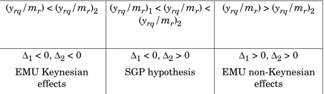
there emerge three different regimes determining the macroeconomic effects, internal and external, of budget variations. They are summarized in the following table.

Table 1. Regimes of fiscal effects

(y_rq/m_r) < (y_rq/m_r)₂ (y_rq/m_r)₁ < (y_rq/m_r) < (y_rq/m_r)₂ (yrq/mr) > (yrq/mr )₂ ∆₁ < 0, ∆₂ < 0 EMU Keynesian effects ∆₁ < 0, ∆₂ > 0 SGP hypothesis ∆₁ > 0, ∆₂ > 0 EMU non-Keynesian effects

In the first regime (first column) budget variations in one country exert Keynesian effects, whereas in the third regime they exert non-Keynesian effects, in the EMU as a whole. The mid-regime combines a Keynesian effect in the originating country with a non-Keynesian one in the other. I call this the "SGP hypothesis" since it figures prominently among the arguments in favour of binding fiscal rules for national FAs (see e.g. Buiter et al. (1993), Eichengreen-Wyplosz (1998), Artis-Winkler (1999)). On the one hand, the argument runs, each government has an incentive to seize the domestic positive effects of budget deficits. On the other, if the financial effects of fiscal imbalances are large, a net negative fiscal spillover may emerge abroad, with a budget deficit in one country exporting a recession in the others. Hence, unfettered budget policies of individual member countries may hurt other members. Table 1 shows that this peculiar SGP hypothesis

is possible within a limited range of parameter values19_{. Clearly, in the}

other regimes the problem underlying the SGP vanishes: in the first regime a budget deficit in one country may also stimulate economic activity in the others, whereas in the third regime no government would ever be tempted to run excessive budget deficits.

The model also points out two factors that may limit the strength of the financial channel of interdependence and hence the extent of negative fiscal spillovers in a currency union. The first concerns the parameter yrq itself. Since yrq ≡ yr + yq(1−α)¸ where (1−α) is the share of flexible-rate extra-EMU trade, yrq is smaller for a country that moves from a flexible exchange-rate regime (where α = 0) into the EMU (where

α > 0). It is also a well-known fact that intra-EMU trade takes a large share of almost all members' international exchanges. The second factor relates to interest rate determination. As shown by equation 0, where the summation of g_i's appears, the impact of a single government's borrowing requirement on the interest rate in a currency union is diluted thanks to the increased market dimension. Moreover, completion of financial integration and participation in a single money market may enhance money-bond substitutability, raise the value of m_r and lower that of the yrq/mr ratio. To be sure, these same factors are often mentioned as possible incentives to budget laxity for individual countries joining the EMU, but it also true that the lower the y_rq/m_r

ratio in each country, the less likely becomes the danger of negative fiscal spillovers for the EMU as a whole.

I do not conclude that negative fiscal spillovers will be a minor problem in the EMU and that fears about this problem are groundless. I contend instead that, though critical for fiscal policy conduct in a currency union, this issue is largely empirical in nature, that it deserves

19_{A (perhaps more realistic) alternative is that the yrq/mr ratio may differ in}

different countries (being small in deficit-prone countries and large in the others). But in this case the problem with the SGP is that setting equal rules for different countries is not efficient (see e.g. Eichengreen-Wyplosz (1998)). The relationship between the y_rq/m_r ratio and the deficit rules in the SGP will also be clarified in the next section.

further accurate investigation, and that it can hardly be settled definitively for all countries and in all circumstances20_{. As the model}

shows, this specific aspect of interdependence in a currency union should be framed within an extended analysis of aspects concerning the transmission mechanism of macroeconomic variables across the EMU, institutional and operational relations between the ECB and the national FAs, and in particular the reciprocal repercussions of their economic policies. These aspects are dealt with in the subsequent parts of this paper.

3. Efficiency of stabilization policies in the EMU

To sum up the preliminary results established in the previous section, when the EMU economies are hit by domestic shocks with a

20_{The empirical literature has hitherto been inconclusive, not to mention the}

facts that genuine data on the EMU are still lacking and that past experiences cannot be translated mechanically into the new institutional and market environment of the EMU. Masson and Taylor (1993) report that estimations run with the IMF world model MULTIMOD support earlier Mundell-Fleming conclusions that fiscal expansions in one country have positive effects on economic activity abroad under a flexible exchange rate (e.g. the US-EEC case in the 1980s) whereas they have negative effects abroad under a fixed exchange rate (e.g. the Germany-EEC case in the 1990s). Using the same model, Hughes Hallet and McAdam (1999) have simulated the process of convergence to balanced budgets in the EMU, finding that domestic fiscal restrictions do not stimulate partners' economic activity, and that a key variable in determining the overall effect on economic activity is the concomitant monetary stance. Allsopp et al. (1999), using the McKibbin-Sachs Global Economic Model (MSG2), by contrast argue that collective fiscal consolidation forced by the SGP is less costly than if individually undertaken, because of the larger positive financial effect of lower interest rate and euro rate depreciation. However this finding does not necessarily imply "non-Keynesian" fiscal spillovers across countries. Eichengreen-Wyplosz (1998) present econometric estimations of an AD-LM-AS model for OECD countries from 1955 to 1996 showing that domestic fiscal coefficients are "Keynesian", whereas external effects are negligible.

certain degree of correlation, these have effects on domestic output and prices, and therefore on EMU output and prices. Consequently, also involved are the common money market, the EMU interest rate and the euro rate. I now examine the stabilization problem faced by the policy makers. In order to focus on the stabilization capacity of the EMU, let us assume that all the policy makers, both central and national, pursue

pure stabilization; that is to say, i) they share the same model of the

economy and the same targets of inflation and potential output, ii) they wish to minimize deviations from target values of inflation and output with no "inflation bias" in their objective functions (they abstain from using macroeconomic policies intended to manipulate the long-run equilibrium levels of inflation, output and unemployment). Moreover, in the presence of demand shocks such that fluctuations in output are positively correlated with those in prices, no policy dilemma arises since stabilization of output and prices are always mutually compatible regardless of the policy-makers' preferences21_{. Therefore, we can simply}

assume that the target of each FA is π_i = 0, and that the target of the ECB is π = 0. As we shall see, even in this ideal regime where all policy-makers are disciplined and face no policy dilemmas, the stabilization problem still presents a few pitfalls that have not been examined carefully in the literature. These depend on three factors highlighted by equations 0-(2.18): i) the interdependence between countries, ii) the degree of correlation of shocks ρ, iii) the "division of labour" among the national fiscal instruments gi and the central monetary one m.

The first question that naturally arises in the face of a shock is: who should stabilize? Note immediately that only two of the target equations 0-(2.18) are linearly independent; since there are three policy instruments in the system (m, g1, g2), one instrument is redundant.

21_{For a formal proof see Appendix A.2. A related analytical advantage is that}

in this context it is unnecessary to specify what the policy-makers’ preferences are.

Hence there can only be two alternative answers to the previous question: either the ECB or the two national FAs22_.

Let us first examine the ECB. It has one instrument, the money supply m, and one target, the EMU inflation rate π, whereas the national targets are two. By setting π = 0, g_i = 0, and solving for m we obtain:

(3.1) m* = −[mr(1+ρ)/2yrq]δ1

(3.2) π1 = (1 −ρ)[2(1+ 2yq + yz)]−1δ1

(3.3) π₂ = −(1 −ρ)[2(1+ 2yq + yz)]−1δ1

Clearly, π_i ≠ 0 for ρ ≠ 1, i.e. national economies are under-stabilized, and their degree of stabilization is an increasing function of the correlation of shocks ρ. The basic reason is that the ECB gears money supply to stabilization of the EMU aggregates, not necessarily of their country components. Therefore, our first conclusion is summarized in the following proposition

(P1) Stabilization assigned to centralized monetary policy is always

effective for the EMU as a whole, but it cannot be effective for all countries unless a symmetric shock occurs (ρ = 1).

This result replicates those of De Grauwe (2000) and Cooper and Kempf (2000) who obtain it for supply-side shocks. De Grauwe relates this result to the interplay between asymmetric shocks and a "representative" ECB's reaction function interpreted as the weighted average of national preferences. Cooper and Kempf obtain it in a traditional context of conflicting targets among policy makers. As is clarified above, the reason behind (P1) is more basic: the lack of instruments vis-à-vis objectives when aysmmetric shocks occur. By contrast, Dixit and Labertini (2001) conclude that in a pure stabilization regime − which they call "monetary-fiscal symbiosis" − centralized monetary policy is always fully stabilizing for both the EMU as a whole

22_{The case of the ECB and one FA can be excluded because it would give rise to}

and for each country for any kind of shock. The main reason is that in their model all countries always have the same EMU inflation rate; hence no problem of incomplete stabilization can ever arise no matter what stabilization policy is chosen. Yet continuous inflation alignment across EMU members is a strong (counterfactual) assumption as far as cyclical fluctuations are concerned. By contrast, proposition (P1) makes it necessary to distinguish the two scenarios of symmetric and asymmetric shocks.

3.1. Symmetric shocks

As far as symmetric shocks are concerned, (P1) seems to be in line with the conventional wisdom: symmetric shocks should be stabilized by the ECB, and the centralized monetary policy may fit all. Yet the alternative assignment to decentralized fiscal stabilization is equally possible. In fact, the national FAs have one instrument, the budget adjustments gi, and one target, the national inflation rate πi, each. Consequently, there always exists a vector of fiscal instruments that completely stabilizes all the economies and the EMU. By setting π_i

= 0, m = 0, in equations 0-(2.18) with ρ = 1 and solving for g_i, we obtain

(3.4) g*₁ = g*2 = [mr/(mr− yrq)]δ1

Should we conclude that in the case of symmetric shocks we are indifferent between monetary and fiscal stabilization? Probably not, as the principle of optimal assignment suggests. Notably, most current analyses of stabilization policies in the EMU do not address this issue.

Let us compare compare the fiscal full-stabilization solution (3.4) with the monetary one provided by equation (3.1) under a symmetric shock

(3.5) m* = −[mr/yrq]δ1

As is well known, in the early Tinbergen-Meade approach, efficient assignment requires that for any target variation dy, the instrument xi that has to be assigned to y should satisfy

Implicit in this assignment principle are considerations on the “cost of the instrument”. Friedman’s famous warning against the “long and variable lags” of policy interventions were of similar nature. More up-to-date considerations, more relevant to stochastic environments, focus on how much of the variability of shocks is transmitted to policy variables. For example, recent studies on the conduct of monetary policy in industrialized countries (e.g. Clarida et al. (1999)) highlight the preference of central bankers for smooth changes in interest rates. Today’s commitment to “price stability” may be extended to asset prices and the exchange rate. In the present model, both monetary and fiscal instruments have repercussions on the EMU interest rate and the euro rate. Using equation 0 we can compute how much variability is transmitted to the interest rate by the two alternative policies. Denoting with σ2_{δ the variance of the shocks, and with σ}2_{r|• the variance of the}

interest rate conditional on one policy instrument, we obtain

σ2_{r|g*i = σ}2_{δ/(mr− yrq)}2

σ2

r|m* = σ2δ/y2rq

In this view, the choice of the stabilization instrument should follow from a minimum variance criterion23_{. Hence, the following}

second proposition holds:

(P2) Under symmetric shocks either central monetary stabilization or

decentralized fiscal stabilization are effective. According to the minumum variance criterion, central monetary stabilization is more efficient if σ2_{r|m* < σ}2_{r|g*i , or yrq /mr > 1/2.}

The condition identified in (P2) is, unsurprisingly, dependent on the y_rq /m_r ratio discussed in section 2 in relation to the financial effects of budget imbalances. For the same reason, it is also akin to the well-known Mundell-Fleming assignment solution in an open economy

23_{Of course, this criterion is only one among many others and is adopted here}

just for expository purposes. It can easily be checked from equations (3.4) and (3.5) that the early criterion of the "minimum use" of the instrument would yield the same result.

with flexible exchange rate. In fact, under symmetric shocks (in a pure stabilization regime) all national FAs behave identically as if there were a single centralized FA, and the y_rq /m_r ratio operates as the Mundell-Fleming open-economy crowding-out parameter (reduced by the share of fixed-rate intra-EMU trade). Consider a negative shock. By raising the EMU interest rate and appreciating the euro rate, an equal fiscal expansion by all governments feeds some crowding-out effect in all the

economies. If this effect is large, the overall extent of fiscal stabilization

should also be larger, and hence the variability of the interest rate turns out to be greater than in the case of monetary stabilization. It also follows that the argument that national fiscal restraints are necessary because negative fiscal spillovers in the EMU are large is consistent with efficient assignment of stabilization to centralized monetary policy in the event of symmetric shocks.

3.2. Asymmetric shocks

We have seen that in case of asymmetric shocks full stabilization for every country cannot be achieved by centralized monetary policy. Consequently, a third proposition follows:

(P3) In the event of asymmetric shocks (ρ < 1), decentralized fiscal

stabilization is the only assignment consistent with full stabilization.

Referring back to the inflation equations 0-(2.18), in consideration of the fiscal spillovers between the two countries discussed in section 2, the decentralized stabilization problem can generally be treated in game-theoretic form. A large body of literature has been produced on comparing co-ordinated with unco-ordinated fiscal stabilization policies among interdependent economies. Generally, unco-ordinated policies in the presence of asymmetric shocks and fiscal spillovers are viewed as being inferior to co-ordinated policies, with positive fiscal spillovers inducing under-stabilization and negative fiscal spillovers incentivating excess deficits (e.g. van der Ploeg (1991), Goodhart-Smith (1993)). Hence those who foresee the former type of fiscal spillover in the EMU warn that decentralized fiscal stabilization may be insufficient, whereas those who are concerned with the latter

type have urged the introduction of budget constraints (see e.g Artis-Winkler (1999)). Yet the majority of recent analyses start from the existence of conflicting interests among national FAs or with the central bank, and/or of some "cost of the instrument" in the use of budget adjustments (see e.g. Buti et al. (2001)). Here the problem can be re-examined in a disciplined system, where policy makers have no conflicting objectives and the cost of budget adjustments may be considered zero up to the SGP deficit ceiling. In this same framework, Dixit and Lambertini (2001) argue that national FAs can always achieve full stabilization whether they co-ordinate or not; however, as noted above, their model does not examine decentralized fiscal stabilization from the efficiency point of view.

In the first place, let us study the unco-ordinated (Nash) equilibrium of the game, where each FA chooses gi in relation to its own national target, taking the FA's choice as given. Under the assumption that π_i = 0 is the target for all FAs, given ρ < 1 and m = 0, the two FAs' reaction functions are reproduced in figure 1. The two functions have the same slope (−∆₂/∆₁), whose sign depends on the prevailing regime of fiscal effects among those in table 1. Figure 1 reproduces the two most representative regimes: the one with EMU Keynesian effects, which implies −∆₂/∆₁ < 0, and the SGP hypothesis, which implies −∆₂/∆₁ > 0.

Figure 1. Fiscal reaction functions and unco-ordinated (Nash) equilibria

A B g 2 g 1 FS1 FS2 A B g2 1 FS1 FS2 g

SGP hypothesis Keynesian regime

After a shock (δ₁, ρδ₁) in the two countries, the unco-ordinated optimal budget adjustments are, respectively,

(3.6) g*₁ = [2m_r− y_rq (1−ρ)][2(m_r− y_rq)]−1_δ1

(3.7) g*₂ = [2mrρ + yrq(1−ρ)][2(mr− yrq)]−1δ1

This outcome prompts some important considerations related to the discussion on fiscal spillovers in section 2.

1) The signs of the optimal budget adjustments are ambiguous in both countries. Once again, we have to examine the y_rq /m_r ratio, and we see that, as far as ρ > 0, y_rq / m_r < 1 is a sufficient condition for (g*₁,

g*₂) to have the same sign as δ₁, i.e. for optimal budget adjustments to be anti-cyclical as traditionally expected. Under these conditions no difference is to be expected from moving from unordinated to

co-ordinated policy choices, the reason being that all governments share the same objective function24_.

2) Two particular cases are worth noting. The first is a unilateral shock, e.g. in country 1, δ₁ < 0, ρ = 0: the result is (g*₁, g*₂) < 0. Note that country 2 should also run a budget deficit just in order to compensate for the imported shock, thereby contributing itself to the overall pressure on the interest rate. The second case is a bilateral trade shift from country 1 to country 2, δ₁ < 0, ρ = −1: the result is g*₁ =

δ₁, g*₂ = −δ₁, i.e. the two countries should exactly offset the change in aggregate demand with an equal budgetary compensation of opposite sign. Consequently, the aggregate borrowing requirement is balanced, and hence no negative financial spillover arises.

We can therefore put forward the following fourth proposition (P4) In the event of asymmeteric shocks of any degree, and for any sign of

fiscal spillovers, if all national FAs consistently pursue the same objective of full stabilization, the unco-ordinated (Nash) equilibrium of their budget choices always achieves both domestic and EMU stabilization.

This conclusion is in line with Dixit and Lambertini's; however, it should be qualified in consideration of the loss of efficiency of decentralized fiscal policies in the presence of negative fiscal spillovers. The condition y_rq / m_r < 1, as established in section 2, admits of both fiscal regimes in figure 1. What is the main difference between the two? It is the extent of budget adjustments. Figure 1 depicts a unilateral negative shock to country 1 (δ1 < 0, ρ = 0): in both fiscal regimes, the

full-stabilization reaction function of government 1 (FS1) shifts downward in the budget deficit region, while that of government 2 (FS2)

24_{In fact, as recalled by van der Ploeg, "international cooperation occurs,}

firstly, through the international exchange of information, secondly, through international harmonization of rules, and thirdly, through international coordination of discretionary policies (1991, p.140). Each government pursuing the same objective function independently corresponds to the second requisite and is a substitute for the third.

also shifts leftward in the deficit region by the amount of the imported shock. Consistently with equations 0-(3.6), the Nash equilibrium shifts from point A to point B where (g*₁, g*₂) < 0 in both fiscal regimes. Yet the absolute value of (g*1, g*2) is different. It increases with ρ and with

the y_rq /m_r ratio. In fact, the former parameter determines the diffusion of the negative shock in the EMU; the latter determines the extent of the crowding-out effect of budget deficits that should be overcome. Therefore, the larger the y_rq /m_r ratio, i.e. the more likely the SGP hypothesis, the larger (more volatile) the optimal budget responses should be in all countries, as a consequence of the fact that decentralized fiscal stabilization loses efficiency also locally.

3.3. A note on the deficit ceiling in the Stability and Growth Pact

From the previus conclusion there follows that the SGP hypothesis, the assignment of asymmetric shocks to decentralized fiscal stabilization and the imposition of budget constraints do not seem mutually consistent. Under the SGP hypothesis, national FAs forced to cope with their own domestic shocks with an inefficient instrument should be granted wider, not narrower, room for anti-cyclical fiscal manoeuvre25_{. To see this more formally, let g}−_{i < 0 be the maximum}

budget deficit compatible with the SGP ceiling for the given observed GDP26_{; consequently, imposing g*} i > g−i and m = 0, then (3.8) ρ − − − ≤ δ −

25_{The advice often offered to governments that they may keep their budget}

slightly positive if they wish to insure themselves against unexpected need for large deficits is extravagant, for aiming at a structurally positive fiscal budget may have distortionary effects which depress the level of potential output.

26_{The SGP ceiling may exceed the normal value of 3% of GDP under certified}

conditions of mild or severe recession: see Buti et al. (1998) for detailed treatment of these provisions.

is the amplitude of the shock that each individual economy can ‘afford’ to accommodate locally without violating the SGP constraint. In particular, (3.8) confirms that if the ECB does not intervene, and if all governments stabilize locally, then |δ_i| decreases (the deficit ceiling is more binding) as the y_rq/m_r ratio grows larger.

A number of exercises and simulations have recently been produced in order to assess the stringency of the SGP constraint (e.g. Buti et al. (1997), Buti-Sapir (1998, chaps. 8-9), Eichengreen-Wyplosz (1998)). These exercises have generally been run on the basis of country-by-country historical data on cyclical slumps and budget responses, and point to the conclusion that the SGP deficit ceiling will probably not be a major impediment to stabilization. However, the institutional regime shift represented by the EMU should be taken into account. Condition (3.8) points out that, in a currency union like the EMU, calculation of the margin of stabilization provided by the SGP cannot be performed by taking the country concerned in isolation. Instead, such calculation must take account of: i) the contemporaneous fiscal position of the other countries in the union, ii) the concomitant monetary stance of the central MA, iii) the correlation of the domestic shock with those in the other member countries. Moreover, little attention has been paid to the consequences of constrained fiscal stabilization.

The SGP deficit ceiling can be seen as a special case of "cost of the instrument" in policy choice-theoretic models. The general result in these models is that when the marginal benefit of stabilization is equated with the marginal cost of the instrument, the latter is used more parsimoniously and hence under-stabilization is the outcome (see e.g. Goodhart-Smith (1993), Buti et al. (2001)). Suppose for simplicity that each government, in the case of negative shock, chooses27

max(g*_i, g−_i)

27_{In this case the fiscal cost function is zero up to g}−_{i and infinite elsewhere.}

More precisely, in this interpretation g−_i may be the maximal contingent deficit below which no ECOFIN procedure is activated.

Suppose also that after a shock the optimal deficit for one government exceeds the ceiling, g*_i < g−_i, while for the other it does not. Then, the former government is constrained to the g−_i deficit. In the light of equations 0-(2.18), there are three main consequences: i) the constrained government under-stabilizes, ii) the unconstrained government can still stabilize domestically by changing its optimal budget choice, iii) the EMU as a whole is under-stabilized.

These three consequences arise in both the fiscal regimes in figure 1 . There is however a major difference as regards the unconstrained government. Under the SGP hypothesis, the unconstrained government will stabilize domestically by choosing a

smaller deficit (because the smaller deficit of the constrained

government exerts a smaller negative fiscal spillover), whereas in the Keynesian regime the optimal deficit should be larger (because the smaller deficit of the constrained government exerts a smaller positive fiscal spillover)28_{. Therefore, if the SGP hypothesis is true, the deficit}

ceiling, when it is binding, enforces the minimization of aggregate deficits (which may be reckoned as a collective benefit) vis-à-vis under-stabilization of the constrained country (which may be reckoned as a private cost). If instead the SGP hypothesis turns out to be untrue, when the deficit ceiling is binding there will still be under-stabilization of the constrained country but no, or negligible, reduction in aggregate deficits. The welfare rationale of both outcomes is unclear, but none of them is a Pareto improvement with respect to the Nash equilibrium of unconstrained stabilization.

28_{The analogous result that stabilization in only one country is less efficient}

than if pursued in all countries has frequently been pointed out in the literature on fiscal policy coordination problems (see e.g. Van der Ploeg (1991), Goodhart-Smith (1993), Abrham et al. (1991)). As we have seen, this principle only holds in so far as fiscal spillovers are positive.