THE DAGUM MODEL OF HUMAN CAPITAL DISTRIBUTION Michele Costa
1. INTRODUCTION
The concept of human capital represents one of the main references of eco-nomic analyses and can be regarded as a key point in development and growth processes (Mulligan and Sala-I-Martin, 2000). Since human capital is a variable which is not directly observable, its measurement symbolizes a challenging trial for researchers and involves both methodological questions and empirical prob-lems (Stroombergen et al., 2002; Wössmann, 2003).
Differently from income, wealth and debt, human capital is a latent variable and, therefore, has to be estimated. The list of researchers interested in human capital estimation is extremely long, it goes back to the 16th century, with the pioneristic work of William Petty and reaches an extraordinary peak in the second half of the 20th century.
Among these researchers Camilo Dagum undoubtedly plays a primary role: in his many contributions to human capital estimation (Dagum, 1994; Dagum and Vittadini, 1996; Dagum and Vittadini, 1997; Dagum, 1999a, b; Dagum and Slottje, 2000; Dagum et al., 2003a, b) different and innovative solutions are proposed and, above all, a model able to describe and interpret human capital distribution is specified.
In this work, by resorting to Dagum’s model, the distribution of human capi-tal, measured by using Wold’s method for latent variables, is analysed on the basis of the information provided by the Bank of Italy’s survey on income and wealth of the Italian households.
2. WOLD’S METHOD FOR HUMAN CAPITAL LATENT VARIABLE
Human capital estimation by means of partial least squares (Cassel et al., 1999; Wold, 1985) represents a special case of a more general method proposed by Wold (1982) with the aim of analysing a set of latent variables and ! on the ba-sis of the observable variables z and y:
z z y y B z y ! " # ! " # " $ % & & % & % &
When the analysis involves only one latent variable , the general specification can be simplified into
y y
y%# "&
where y is the vector of the q observable variables used for the human capital estimation.
By denoting with x and ' the variables y and in deviation form, it is possible to obtain the latent variable ' as a weighted mean of the observable indicators x
1 q i i i w x ( % %
)
In order to estimate ', Wold suggests an iterative procedure where initial val-ues wi0 are set equal to 1, thus allowing to calculate the first approximation of ':
0 1 q i i x ( % %
)
The values (0 are then standardized to give unit variance
0 1 0/ '
( %' * . The
first iteration is then completed with the ordinary least squares estimation of the coefficients wi1 in the relation
1 1 1 1 q i i i w x ' ( " % %
)
&From the estimates wi1 a new approximation of ' is calculated and the itera-tion proceeds until the values wi converge with respect to some conventional stopping rule, such as
5 1
(wih wih)/wih 10 i
+
& + - ,
Since the variables x and ' used in the procedure which calculates the weights i
w are in deviation form, the last step of Wold’s method concerns the mean value of the latent variable . This value can be easily achieved by means of the following relation 1 q i i i w y % %
)
.Finally, by moving from y and it is possible to derive the coefficients #y and also other results related to the framework of partial least squares. The focus of this work is represented by the information which Dagum’s model is able to ex-tract from latent variable .
3. THEL DAGUM GENERAL MODEL
Dagum (1977, 1990, 1993, 1994) specifies a general model which, according to a set of ideal properties, is able to describe and interpret the human capital distri-bution, besides the income, wealth and debt distributions.
The general model is a mixture of three functions and can be expressed as
1 1 2 2 3 3 1 2 3 1 2 3 ( ) ( ) ( ) ( ) , 0, 1, 0, 1 F x b F x b F x b F x b b b b b b % & & . / 0 & & %
with the following analytic specification:
1 2 3 1 2 3 1 2 1 2 3 ( ) exp( ) max 0; (1 ) , 0 e 0 0, 0 e 0 0, 0, 1, 0, , 1, ( , , , ) 0, 1. s x F x b c x b b x x x x x x x x x x x b b b b b b b b c s 1 2 3 2 # 1 # + + + & + + , & & , 4 5 6 6
% + & 8 9& & +7 / / 7
6 6
: ;
< / % . < 0 %
-. / 0 & % & & % 0 0
The density function of the model is:
1 1 1 1 2 2 3 ( ) ( ) dF x | | exp( |s | )s (0) (1 ) f x b cs x c x b f b x x dx 1 1 2 2# 1 # + + + + + + + + & &
% % + & & &
where 1 1 1 1 ( ) | | ( ) | | exp( | | ) | | s s dF x d x f x b c s x c x d x dx + + + % % + 1( ) 0 f x % , ,x 0 0 2(0) 1 f % , and f x2( +)% f x2( &) 0% 1 1 3 3 ( ) ( ) dF x (1 ) f x x x dx 1 1 2 2 # 1 + + # + + + & & % % & , f x %3( ) 0, ,x- . 0
To deal with human capital (Dagum and Costa, 2000), the support of the model is represented by the interval [ , )0 7 , with 0 0 ; this implies 0 b %1 0,
2
From the general model, for the human capital distribution it is possible to de-duce a four parameters specification:
0 0 ( ) (1 )(1 ) , 0, ( , ) 0, 1, 0, e ( ) 0, . F F 1 2 3 3 # 2 # 1 3 + + % & + & . 0 0 0 / % ,
-Since F( ) 00 % , it follows that
0
(1 )(1 1) 2 0
3& +3 &# + + % and then that
1/ 1/ 1/ 0 1 1 1 0, 0 1 2 1 # 3 3 + =? @ > % ACE + DF + B 0 / A B G H
Parameters 3, 2 and 1 are inequality parameters, invariant with respect to the unit of measurement, while # is a scale parameter.
More specifically, parameter 3 represents the frequency of units with human capital 0.
Furthermore, from the estimate of 1 it is possible to deduce the number of fi-nite moments of the fitted human capital distribution. This information is highly relevant for the debate on the role of the distributions with infinite variance as models for economic variables such as income, wealth, debt and human capital. Empirical evidence does not always support the hypothesis of infinite variance and also suggests the existence of finite moments of order greater than one. The Dagum model allows, for 1I< 2, the case of infinite variance and, for higher val-ues of 1, the case of finite moments of higher order. Therefore, by increasing val-ues of 1, the human capital distribution, for J 7 , shows a faster convergence to 0. Dancelli (1986) proves that parameter 1 is sensitive to the frequency of units with high human capital, while 2 is sensitive to the frequency of units with low – medium human capital.
Also the product 21Igives powerful insights on human capital, since it der-mines whether the distribution of is zeromodal or unimodal: when 0/21 - 1 the fitted distribution is zeromodal and when 21 0 is unimodal. The flexibility 1 with respect to both zeromodal and unimodal distributions represents a main fea-ture of Dagum model, which is able to evaluate the two different situations, both present in empirical researches and with a deep impact on the inequality charac-teristics of the analyzed variable.
Finally, the last fundamental element of Dagum’s model refers to its capability to deduce the Lorenz curve and to calculate the Gini index G as a function of inequality parameters 3KI2Iand 1
G = G(3K2K1)
where G is an increasing function of 3 and a decreasing function of 2IandI1I
/ 0, / 0, / 0.
G 3 G 2 G 1
L L 0 L L / L L / I
4. DATA AND OBSERVABLE INDICATORS
The analysis of human capital is performed by referring to the data of the Bank of Italy survey on Italian households income and wealth. (Brandolini, 1999; Bran-dolini and Cannari, 1994; D’Alessio et al., 2004).
The reference period goes from 1993 to 2004 and includes the six surveys per-formed in the last years: 1993, 1995, 1998, 2000, 2002 and 2004.
The choice of observable indicators requires to deal with a problem still un-solved in the wide literature on human capital: the theoretical discussion has not yet univocally defined the optimal set of observed variables which are to be in-cluded for the human capital estimation. In the following, the focus is on the variables measured in monetary units, in particular income, real wealth, debt and financial wealth. Since data about financial wealth are not available for the less recent surveys, this variable is not included in the analysis and only for the year 2004 results with and without financial wealth are compared.
By assuming the household as statistical unit, some descriptive statistics related respectively to income, real wealth and debt of the Italian households are re-ported in Tables 1-3.
TABLE 1
Real wealth of Italian households from 1993 to 2004, thousand euro
1993 1995 1998 2000 2002 2004 Number of observations 8089 8135 7147 8001 8011 8012 Mean 108730 119476 131105 141836 158283 187410 Median 62491 73344 78243 82633 100000 121000 Variation coefficient 1.75 1.83 2.25 1.86 1.66 1.70 Kurtosis 195.64 330.64 1487.64 132.08 75.00 117.68 Asymmetry 9.67 12.65 27.28 8.72 6.55 8.30 TABLE 2
Income of Italian households from 1993 to 2004, thousand euro
1993 1995 1998 2000 2002 2004 Number of observations 8089 8135 7147 8001 8011 8012 Mean 20431 22112 24930 26099 27868 29483 Median 16578 18070 20272 21397 22986 23833 Variation coefficient 0.75 0.79 0.87 0.79 0.77 0.87 Kurtosis 23.35 54.25 83.60 54.92 44.59 270.78 Asymmetry 2.87 4.48 5.86 4.53 4.08 10.01
TABLE 3
Debt of Italian households from 1993 to 2004, thousand euro
1993 1995 1998 2000 2002 2004 Number of observations 8089 8135 7147 8001 8011 8012 Mean 3226 3554 4162 6080 6282 8699 Median 0 0 0 0 0 0 Variation coefficient 4.53 4.35 12.69 5.27 3.94 7.14 Kurtosis 285.93 241.25 3043.64 2293.12 87.86 3038.41 Asymmetry 13.37 11.74 51.28 32.79 7.74 48.01
Real wealth and income show the usual features which characterize, in devel-oped countries, the distribution of these variables: positive asymmetry and high kurtosis, as the result of the presence of some households with extremely high values for both variables. Furthermore, the real wealth distribution presents, as typical, a higher variation coefficient than the income, thus confirming its greater variability. Finally, in the debt distribution, it is possible to observe, besides the usual high frequency of households without debt, a strong increase in the house-hold mean debt from 1993 to 2004.
5. HUMAN CAPITAL IN ITALY, 1993 - 2004
Dagum’s four parameter model is applied to the values of latent variable hu-man capital obtained by means of Wold’s method. The parameter estimates are achieved by resorting to an iterative procedure implemented in EPID software (Dagum and Chiu, 1991). The use of a model able to describe and interpret hu-man capital distribution is a relevant step in order to detect the main features of human capital and also allows to overcome, at least partially, the difficulties re-lated to the many alternatives available for the choice of the observed variables.
In Table 4 Dagum’s model parameter estimates are reported for the 2004 hu-man capital distribution. The set of observable indicators in the second column consists of income, real wealth, debt and financial wealth, while in the third col-umn financial wealth is omitted.
TABLE 4
Dagum model estimates for human capital distribution in Italy, 2004, with and without financial wealth
2004 With financial wealth Without financial wealth
3 -0.099 -0.124 2I 0.421 0.362 # 5.697 6.052 1 2.655 2.850 Gini index 0.498 0.489 SSE(CDF) 0.0005 0.0008 SSE(PDF) 0.0006 0.0009
From Table 4 it is possible to deduce how different sets of observable indica-tors can influence both human capital values and Dagum’s model estimates. In order to allow for a correct comparison from 1993 to 2004 the set of observed indicators is restricted to income, real wealth and debt and in Table 5 the
parame-ter estimates are reported as well as a selection of statistics for Dagum model ap-plied to human capital distribution of Italian households.
In the lower panel of Table 5, after the number N of observations used in the model estimation, it is possible to notice the extremely low values of the sums of square errors of probability density function (PDF) and cumulative density func-tion (CDF) as well as of the Kolmogorov – Smirnov statistic, which suggests an excellent goodness of fit of the Dagum model.
TABLE 5
Dagum 4 parameter model estimates and summary statistics for Italian households human capital distribution from 1993 to 2004 1993 1995 1998 2000 2002 2004 3 -0.063 -0.108 -0.036 -0.043 -0.067 -0.124 b3 =1-3 1.063 1.108 1.036 1.043 1.067 1.124 2 0.441 0.346 0.495 0.564 0.485 0.362 # 7.038 8.093 2.626 3.324 4.882 6.052 1 2.714 2.862 2.770 2.564 2.570 2.850 21 1.20 0.99 1.37 1.45 1.25 1.03 0 0.1949 0.1980 0.1232 0.1760 0.2020 0.2219 Gini index 0.481 0.488 0.458 0.480 0.494 0.489 N 39 39 39 39 39 39 SSE (CDF) 0.0003 0.0003 0.0004 0.0003 0.0003 0.0008 SSE (PDF) 0.0003 0.0005 0.0005 0.0003 0.0002 0.0009 K-S 0.0007 0.0008 0.0008 0.0006 0.0006 0.0014 Diff. mean -1.94% -0.62% 1.38% -0.11% -1.65% 0.15% Diff. median -0.77% -0.39% -0.97% -0.75% -0.79% -0.03% -2 -1,5 -1 -0,5 0 0,5 1 1,5 2 1993 1995 1998 2000 2002 2004
Figure 1 – Dagum model for human capital distribution in Italy from 1993 to 2004. Per cent differ-ences between observed and estimated values for the mean (continuous line) and the median (dotted line).
The differences between observed and estimated values for both mean and median, also illustrated in Figure 1, are always quite small, thus confirming the goodness of fit of the model. In particular, the differences for the median are constantly smaller than 1%, while the differences for the mean range between -1.94% and -0.11%.
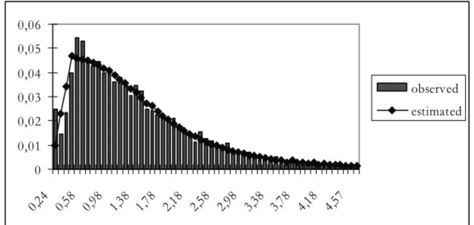
Figure 2 shows the observed data for the year 2004 and the estimated values obtained by means of Dagum model. Human capital distribution is fitted with great precision for both initial values and highest values. Furthermore, with re-spect to the year 2004, it is possible to observe a near zeromodal distribution, with an extremely steep first section of the curve.
0 0,01 0,02 0,03 0,04 0,05 0,06 0,24 0,58 0,98 1,38 1,78 2,18 2,58 2,98 3,38 3,78 4,18 4,57 observed estimated
Figure 2 – Dagum model for human capital in Italy, 2004, observed data and estimated values. From the parameter estimates reported in Table 5 it is possible to observe how the product 21 results smaller than one only for 1995, while, for the remaining years, it is 21 > 1. Therefore, the fitted human capital distribution is zeromodal for 1995 and unimodal for 1993, 1998, 2000, 2002 and 2004.
Furthermore, the estimates of parameter 1 result greater than two for all the six surveys analyzed in this paper, thus indicating that the fitted distribution has finite variance, while the moments of order r > 1 are infinite.
Finally, the frequency of units with minimum human capital 0, measured by 3
parameter, takes values included between 3.6% for 1998 and 12.4% for 2004, reaching the top values in 1995, when the fitted distribution is zeromodal, and in 2004, when 21 is near unity.
The Gini index fluctuates around the value 0.48, reaching the minimum value of 0.458 in 1998 and the maximum value of 0.494 in 2002.
In order to evaluate the effect of the units with minimum human capital on to-tal inequality, in Figure 3 the Gini index is illustrated, as well as parameter 3KIwith
G being a monotonic increasing function of 3: LG/L30 . 0
It is possible to observe how low values of 3 contribute to reduce inequality, while, on the contrary, high frequencies of units with minimum human capital lead to an increase in the Gini index: in 1998 and 2000, when 3 reaches its mini-mum values, also the Gini index reaches its lowest level, while, in 1995 and in 2004, when 3 exceeds 10%, the Gini index shows an increase.
0,44 0,45 0,46 0,47 0,48 0,49 0,5 1993 1995 1998 2000 2002 2004 0 2 4 6 8 10 12 14 Gini alfa
Figure 3 – Dagum model for human capital in Italy from 1993 to 2004, Gini index and 3 parameter.
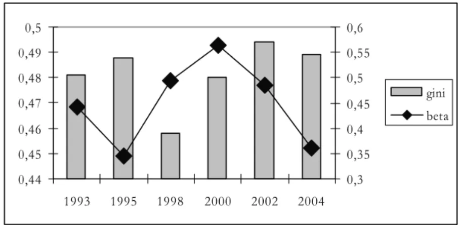
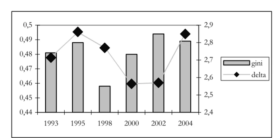
Still for the purpose to evaluate the effects of Dagum model parameters on to-tal inequality, Figures 4 and 5 illustrate the Gini index and, respectively, parame-ters 2 and 1.
The Gini index is a monotonic decreasing function of both parameters 2 and 1
(LG/L2 /0, LG/L1 / ), but, as it is possible to note from Figures 4 and 5, it 0 is not easy to separate the single effects of 2 and 1 on total inequality.
0,44 0,45 0,46 0,47 0,48 0,49 0,5 1993 1995 1998 2000 2002 2004 0,3 0,35 0,4 0,45 0,5 0,55 0,6 gini beta
0,44 0,45 0,46 0,47 0,48 0,49 0,5 1993 1995 1998 2000 2002 2004 2,4 2,5 2,6 2,7 2,8 2,9 gini delta
Figure 5 – Dagum model for human capital in Italy from 1993 to 2004, Gini index and 1 parameter.
Finally, Figure 6 illustrates the fitted human capital distributions for the Italian households from 1993 to 2004. 0 0,01 0,02 0,03 0,04 0,05 0,06 0 1 2 3 4 5 1993 1995 1998 2000 2002 2004
Figure 6 – Dagum four parameter model for human capital of Italian households from 1993 to 2004. It is possible to observe, besides the typical positive asymmetric shape of hu-man capital distribution, both the zeromodal situation of 1995 and the near ze-romodal case of 2004.
6. CONCLUSIONS
The analysis of human capital distribution by means of Dagum’s four parame-ter model achieves the primary aim of identifying the main characparame-teristics of this latent variable. Furthermore, the Dagum’s model allows both to achieve parame-ters with a specific economic significance and to reconcile economic theory with empirical evidence. The results obtained indicate that from 1993 to 2004 the
con-centration ratio of Italian households human capital is quite stable; however, units with minimum human capital 0 play a relevant role, with a strong increase in
their frequency from 2002, F( 0)=6.7%, to 2004, F( 0)=12.4%. Also the
contri-bution related to units with high levels of human capital, measured by the pa-rameter 1, takes on a central meaning in 2004.
On the whole, the model shows an excellent fit to observed data and, confirm-ing the results of previous researches, it proves to represent an efficiente tool for the quantitative analysis of human capital.
Dipartimento di Scienze Statistiche “Paolo Fortunati” MICHELE COSTA
Università di Bologna
REFERENCES
A. BRANDOLINI(1999), The distribution of personal income in post-war Italy: source, description, data
quality and the time pattern of income inequality, “Temi di discussione”, n. 350, Banca
d’Italia.
A. BRANDOLINI, L. CANNARI (1994), Methodological appendix: the Bank of Italy’s survey of household
income and wealth, in A. Ando, L. Guiso e I. Visco (eds.), “Saving and the Accumulation
of Wealth: Essays on Italian Household and Government Saving Behavior”, Cam-bridge University Press, CamCam-bridge, UK, pp. 369-386.
C. CASSEL, P. HACKL, A.H. WESTLUND(1999), Robustness of partial least-squares method for estimating
latent variable quality structures, “Journal of Applied Statistics”, 26, pp. 435-446.
G. D’ALESSIO, I. FAIELLA, A. NERI (2004), Italian households budgets in 2002, “Supplements to the Statistical Bullettin (new series)”, n. 12, Banca d’Italia.
C. DAGUM (1977), A new model of personal income distribution: specification and estimation, “Economie Appliquée”, 30, pp. 413-436.
C. DAGUM(1990), A model of wealth distribution specified for negative, null and positive wealth, in C. Dagum, M. Zenga (eds.), “Income and wealth distribution, inequality and poverty”, Springer-Verlag, Berlin, D, pp. 42-56.
C. DAGUM(1993), A general model of net wealth, total wealth and income distribution, “Proceedings of the American Statistical Association, Business and Economics Statistics Section, 153th meeting”, pp. 80-85.
C. DAGUM(1994), Human capital, income and wealth distribution models and their applications to the
USA, “Proceedings of the American Statistical Association, Business and Economics Statistics Section, 154th meeting”, pp. 91-96.
C. DAGUM(1999a), A study on the distributions of income, wealth, and human capital, “Revue eu-ropeenne des sciences sociales”, 37, pp. 231-268.
C. DAGUM(1999b), Measuring the level of personal and national human capital, “Proceedings of the American Statistical Association, Government Statistics and Social Statistics Sections, 159th meeting”, pp. 1-10.
C. DAGUM, K. CHIU(1991), User's Manual of the Program EPID (Econometric Package for Income
Distribution), Statistics Canada, Ottawa.
C. DAGUM, M. COSTA(2000), Analisi statistica di variabili economiche: un modello generale. Le distri-
buzioni del capitale umano, della ricchezza, del reddito e del debito, “Statistica”, 60, pp. 611-634.
C. DAGUM, D.J. SLOTTJE(2000), A new method to estimate the level and distribution of household
C. DAGUM, G. VITTADINI(1996), Human capital measurement and distribution, “Proceedings of the American Statistical Association, Business and Economics Statistics Section, 156th meeting”, pp. 194-199.
C. DAGUM, G. VITTADINI(1997), Estimation and distribution of human capital with applications, “Scritti di statistica economica”, 3, pp. 115-131.
C. DAGUM, G. VITTADINI, M. COSTA, P. LOVAGLIO(2003a), A multiequational recursive model of
hu-man capital, income and wealth of households with application, Business and Economics
Statis-tics Section [CD-ROM], American Statistical Association, Alexandria, VA.
C. DAGUM, G. VITTADINI, P. LOVAGLIO, M. COSTA(2003b), An estimation methodology for variable
“human capital” in the U.S.A., Business and Economics Statistics Section [CD-ROM],
American Statistical Association, Alexandria, VA.
L. DANCELLI(1986), Tendenza alla massima e alla minima concentrazione nel modello di distribuzione
del reddito personale di Dagum, in “Scritti in onore di Francesco Brambilla”, 1, edizioni
Bocconi, Milano, pp. 249-267.
C.B. MULLIGAN, X. SALA-I-MARTIN(2000), Measuring aggregate human capital, “Journal of Eco-nomic Growth”, 5, pp. 215-252.
W. PETTY (1690), Political arithmetick, III edizione, Archive of the History of Economic Thought, McMaster University, Canada.
A. STROOMBERGEN, D. ROSE, G. NANA(2002), Review of the statistical measurement of human capital, Statistics New Zealand, Wellington.
H. WOLD (1982), Soft modelling: the basic design and some extensions, in K.G. Jöreskog, H. Wold (eds.), “System Under Indirect Observation: Causality, Structure, Prediction”, 2, pp. 1-54. H. WOLD(1985), Partial least squares, in S. Kotz, N. Johnson (eds.), “Encyclopedia of
Statis-tical Sciences”, 6, Wiley, New York, pp. 581-591.
L. WÖSSMANN(2003), Specifying human capital, “Journal of Economic Surveys”, 17, pp. 239-270.
RIASSUNTO
Il modello di Dagum per la misura del capitale umano
Nel lavoro viene illustrata la stima della distribuzione del capitale umano mediante il ri-corso al modello di Dagum. L’analisi fa riferimento al capitale umano delle famiglie italia-ne, misurato con il metodo di Wold per le variabili latenti sulla base dei dati dell’indagine della Banca d’Italia, per il periodo 1993 - 2004. Il modello di Dagum consente di cogliere le caratteristiche fondamentali della distribuzione del capitale umano e permette una in-terpretazione dei parametri in grado di riconciliare teoria economica ed evidenza empirica.
SUMMARY
The Dagum model of human capital distribution
In this paper the estimation of human capital distribution is obtained by means of Dagum model. The analysis refers to Italian households human capital, measured by resorting to Wold’s latent variables method, on the basis of micro data provided by the Bank of Italy’s survey of household income and wealth. The Dagum model allows both to achieve parameters with a specific economic significance and to reconcile economic theory with empirical evidence.