Two-phase flow measurement for SPES3 facility: Spool piece mathematical correlations

(1)

(2)

Via Nino Bixio, 27 - 29100 Piacenza (I) CLIENTE: Client :

ENEA

COMMESSA: job:

1PN000CA90245

DISCO: disk:

CA90245/1

PAGINA: page: 1 DI: of 127 IDENTIFICATIVO: document:

01 572 RT 09

Classe Ris.: Confidential: ALLEGATI: Enclosures: TITOLO:

Title:

TWO-PHASE FLOW MEASUREMENT FOR SPES3 FACILITY:

SPOOL PIECE MATHEMATICAL CORRELATIONS

REDATTORI:

A. Achilli, M. Greco

prepared by:

LISTA DI DISTRIBUZIONE

distribution list

ENEA Renato Tinti

ENEA Fosco Bianchi

SIET S.p.A. Andrea Achilli

SIET S.p.A. Gustavo Cattadori

SIET S.p.A. Stefano Gandolfi

SIET S.p.A. Matteo Greco

SIET S.p.A. Roberta Ferri

SIET S.p.A. Gaetano Tortora

SIET S.p.A. Cinzia Congiu

Rev.0 14/07/2010 Emissione A. Achilli M. Greco G.Cattadori REV. Rev. DATA date DESCRIZIONE description REDAZIONE prepared by APPROVAZIONE approved by

Informazioni strettamente riservate di proprietà SIET SpA - Da non utilizzare per scopi diversi da quelli per cui sono state fornite.

(3)

(4)

Volumetric model - ADS Stage-I DT line, DVI break test... 77 Table 6.10: Errors per cent between the RELAP5 mass flow and the Spool Piece mass flow - Rouhani model - EBT SPLIT line, EBT break test ... 78 Table 6.11: Errors per cent between the RELAP5 mass flow and the Spool Piece mass flow - Aya model - EBT SPLIT line, EBT break test... 80 Table 6.12: Errors per cent between the RELAP5 mass flow and the Spool Piece mass flow - Volumetric model - EBT SPLIT line, EBT break test... 81 Table 6.13: Errors per cent between the RELAP5 mass flow and the Spool Piece mass flow - Rouhani model - ADS Stage-I ST line, EBT break test... 82 Table 6.14: Errors per cent between the RELAP5 mass flow and the Spool Piece mass flow - Aya model – ADS Stage-I ST line, EBT break test ... 83 Table 6.15: Errors per cent between the RELAP5 mass flow and the Spool Piece mass flow - Volumetric model - ADS ST (stage I) line, EBT break test ... 84 Table 6.16: Errors per cent between the RELAP5 mass flow and the Spool Piece mass flow - Rouhani model - ADS Stage-I DT line, EBT break test ... 85 Table 6.17: Errors per cent between the RELAP5 mass flow and the Spool Piece mass flow - Aya model – ADS Stage-I DT line, EBT break test ... 86 Table 6.18: Errors per cent between the RELAP5 mass flow and the Spool Piece mass flow - Voluemetric model - ADS Stage-I DT line, EBT break test... 87 Table 6.19: Errors per cent between the RELAP5 mass flow and the Spool Piece mass flow - Rouhani model - ADS SPLIT line, ADS break test ... 88 Table 6.20: Errors per cent between the RELAP5 mass flow and the Spool Piece mass flow - Aya model - ADS SPLIT line, ADS break test... 90 Table 6.21: Errors per cent between the RELAP5 mass flow and the Spool Piece mass flow - Volumetric model - ADS SPLIT line, ADS break test... 91 Table 6.22: Errors per cent between the RELAP5 mass flow and the Spool Piece mass flow - Rouhani model - ADS Stage-I DT line, ADS break test ... 92

(8)

Table 6.23: Errors per cent between the RELAP5 mass flow and the Spool Piece mass flow - Aya model – ADS Stage-I DT line, ADS break test... 94 Table 6.24: Errors per cent between the RELAP5 mass flow and the Spool Piece mass flow - Volumetric model - ADS Stage-I DT line, ADS break test ... 95 Table 8.1: List of variables derived by [4] upstream and downstream of the break... 108 Table 8.2: Different case analysed for the determination of the relationships between the density ratio and the other thermal-hydraulic variables... 112

(9)

LIST OF FIGURES

Figure 3.1: SPES3 DVI-B break line nodalization... 22

Figure 3.2: SPES3 EBT-B break line nodalization... 23

Figure 3.3: SPES3 ADS ST and ADS Stage-I ST break line nodalization (top view) ... 24

Figure 3.4: SPES3 ADS Stage-I DT nodalization (top view)... 25

Figure 5.1: Comparison between the RELAP5 and theoretical mass flow, void fraction and quality in DVI SPLIT break line, DVI Test... 36

Figure 5.2: Comparison between the RELAP5 and theoretical mass flow, void fraction and quality in ADS Stage-I ST line, DVI Test ... 36

Figure 5.3: Comparison between the RELAP5 and theoretical mass flow, void fraction and quality in ADS Stage-I DT line, DVI Test... 37

Figure 5.4: Comparison between the RELAP5 and theoretical mass flow, void fraction and quality in EBT SPLIT break line, EBT Test... 37

Figure 5.5: Comparison between the RELAP5 and theoretical mass flow, void fraction and quality in ADS Stage-I ST line, EBT Test ... 38

Figure 5.6: Comparison between the RELAP5 and theoretical mass flow, void fraction and quality in ADS Stage-I DT line, EBT Test... 38

Figure 5.7: Comparison between the RELAP5 and theoretical mass flow, void fraction and quality in ADS SPLIT break line, ADS Test... 39

Figure 5.8: Comparison between the RELAP5 and theoretical mass flow, void fraction and quality in ADS Stage-I DT line, ADS Test ... 39

Figure 5.9: Comparison between the RELAP5 and theoretical mass flow, flow regimes and presence of critical flow in DVI SPLIT beak line, DVI Test ... 40

Figure 5.10: Comparison between the RELAP5 and theoretical mass flow, flow regimes and presence of critical flow in ADS ST stage I line, DVI Test ... 41

Figure 5.11: Comparison between the RELAP5 and theoretical mass flow, flow regimes and presence of critical flow in ADS DT stage I line, DVI Test ... 41

Figure 5.12: Comparison between the RELAP5 and theoretical mass flow, flow regimes and presence of critical flow in EBT SPLIT beak line, EBT Test ... 42

Figure 5.13: Comparison between the RELAP5 and theoretical mass flow, flow regimes and presence of critical flow in ADS Stage-I ST line, EBT Test... 42

Figure 5.14: Comparison between the RELAP5 and theoretical mass flow, flow regimes and presence of critical flow in ADS Stage-I DT line, EBT Test ... 43

Figure 5.15: Comparison between the RELAP5 and theoretical mass flow, flow regimes and presence of critical flow in ADS SPLIT beak line, ADS Test... 43

(10)

Figure 5.16: Comparison between the RELAP5 and theoretical mass flow, flow regimes and

presence of critical flow in ADS Stage-I DT line, ADS Test ... 44

Figure 5.17: Comparison between the mass flow rate obtained by the coupling of two instruments (DD + Void) and the RELAP5 mass flow rate in the DVI SPLIT line, DVI break test ... 48

Figure 5.18: Errors per cent function of the slip ratio at 7 bars with quality set to 0.7... 60

Figure 6.1: Comparison between the RELAP5 mass flow and the Spool Piece mass flow - Rouhani model -DVI SPLIT line, DVI break test... 64

Figure 6.2: Comparison between the RELAP5 mass flow and the Spool Piece mass flow - Aya model - DVI SPLIT line, DVI break test... 66

Figure 6.3: Comparison between the RELAP5 mass flow and the Spool Piece mass flow - Volumetric model - DVI SPLIT line, DVI break test... 68

Figure 6.4: Comparison between the RELAP5 mass flow and the Spool Piece mass flow - Rouhani model - ADS Stage-I ST line, DVI break test ... 70

Figure 6.5: Comparison between the RELAP5 mass flow and the Spool Piece mass flow - Aya model - ADS Stage-I ST line, DVI break test ... 72

Figure 6.6: Comparison between the RELAP5 mass flow and the Spool Piece mass flow - Volumetric model - ADS Stage-I ST line, DVI break test ... 73

Figure 6.7: Comparison between the RELAP5 mass flow and the Spool Piece mass flow - Rouhani model - ADS Stage-I DT line, DVI break test... 74

Figure 6.8: Comparison between the RELAP5 mass flow and the Spool Piece mass flow - Aya model - ADS DT (stage I) line, DVI break test ... 76

Figure 6.9: Comparison between the RELAP5 mass flow and the Spool Piece mass flow - Volumetric model - ADS Stage-I DT line, DVI break test... 77

Figure 6.10: Comparison between the RELAP5 mass flow and the Spool Piece mass flow - Rouhani model - EBT SPLIT line, EBT break test ... 79

Figure 6.11: Comparison between the RELAP5 mass flow and the Spool Piece mass flow - Aya model - EBT SPLIT line, EBT break test... 80

Figure 6.12: Comparison between the RELAP5 mass flow and the Spool Piece mass flow - Volumetric model - EBT SPLIT line, EBT break test... 81

Figure 6.13: Comparison between the RELAP5 mass flow and the Spool Piece mass flow - Rouhani model - ADS Stage-I ST line, EBT break test... 82

Figure 6.14: Comparison between the RELAP5 mass flow and the Spool Piece mass flow - Aya model – ADS Stage-I ST line, EBT break test ... 83

Figure 6.15: Comparison between the RELAP5 mass flow and the Spool Piece mass flow - Volumetric model - ADS Stage-I ST line, EBT break test ... 84

(11)

Figure 6.16: Comparison between the RELAP5 mass flow and the Spool Piece mass flow -

Rouhani model - ADS Stage-I DT line, EBT break test ... 85 Figure 6.17: Comparison between the RELAP5 mass flow and the Spool Piece mass flow - Aya model – ADS Stage-I DT line, EBT break test ... 86 Figure 6.18: Comparison between the RELAP5 mass flow and the Spool Piece mass flow -

Volumetric model – ADS Stage-I DT line, EBT break test ... 87 Figure 6.19: Comparison between the RELAP5 mass flow and the Spool Piece mass flow -

Rouhani model - ADS SPLIT line, ADS break test ... 89 Figure 6.20: Comparison between the RELAP5 mass flow and the Spool Piece mass flow - Aya model - ADS SPLIT line, ADS break test... 90 Figure 6.21: Comparison between the RELAP5 mass flow and the Spool Piece mass flow -

Volumetric model - ADS SPLIT line, ADS break test... 91 Figure 6.22: Comparison between the RELAP5 mass flow and the Spool Piece mass flow -

Rouhani model - ADS Stage-I ST line, ADS break test ... 92 Figure 6.23: Comparison between the RELAP5 mass flow and the Spool Piece mass flow - Aya model - ADS Stage-I DT line, ADS break test ... 94 Figure 6.24: Comparison between the RELAP5 mass flow and the Spool Piece mass flow -

Volumetric model - ADS Stage-I DT line, ADS break test ... 95 Figure 7.1: Comparison between the RELAP5 quality and void fraction in volume 667030000 versus the quality and void fraction obtained by the homogenous model, DVI SPLIT break line, DVI break test. ... 104 Figure 7.2: Comparison between the RELAP5 quality and void fraction in volume 134010000 versus the quality and void fraction obtained by the homogenous model, ADS Stage-I ST line, DVI break test. ... 105 Figure 7.3: Comparison between the RELAP5 quality and void fraction in volume 644030000 versus the quality and void fraction obtained by the homogenous model, EBT SPLIT break line, EBT break test. ... 106 Figure 8.1: Upstream void fraction versus the ratio between the upstream and downstream mixture density in CASE 1. ... 113 Figure 8.2: Upstream quality versus the ratio between the upstream and downstream mixture density in CASE 1. ... 113 Figure 8.3: Upstream mixture density versus the ratio between the upstream and downstream mixture density in CASE 1. ... 114 Figure 8.4: Downstream void fraction versus the ratio between the upstream and downstream mixture density in CASE 1. ... 114 Figure 8.5: Downstream quality versus the ratio between the upstream and downstream mixture density in CASE 1. ... 115

(12)

Figure 8.6: Downstream mixture density versus the ratio between the upstream and downstream mixture density in CASE 1. ... 115 Figure 8.7: Upstream Void Fraction versus the ratio between the upstream and downstream

mixture density in CASE 2. ... 116 Figure 8.8: Upstream Quality versus the ratio between the upstream and downstream mixture density in CASE 2. ... 116 Figure 8.9: Upstream Mixture Density versusthe ratio between the upstream and downstream mixture density in CASE 2. ... 117 Figure 8.10: Downstream Void Fraction versus the ratio between the upstream and downstream mixture density in CASE 2. ... 117 Figure 8.11: Downstream Quality versus the ratio between the upstream and downstream mixture density in CASE 2. ... 118 Figure 8.12: Downstream Mixture Density versus the ratio between the upstream and downstream mixture density in CASE 2. ... 118 Figure 8.13: Upstream and downstream pressure and mass flow in the DVI SPLIT break line, DVI break test. ... 120 Figure 8.14: Comparison between the RELAP5 quality and the calculated quality downstream of the break during the DVI break test in the DVI SPLIT line... 121 Figure 8.15: Comparison between the RELAP5 quality and the calculated quality downstream of the break during the DVI break test in the DVI SPLIT line... 121 Figure 8.16: Upstream and downstream pressure and mass flow in the EBT SPLIT break line, EBT break test. ... 123 Figure 8.17: Comparison between the RELAP5 quality and the calculated quality downstream of the break during the EBT break test in the EBT SPLIT line... 124 Figure 8.18: Comparison between the RELAP5 quality and the calculated quality downstream of the break during the EBT break test in the EBT SPLIT line... 124

(13)

LIST OF ACRONYMS

ADS Automatic Depressurization System

Aya Aya model for the Turbine flowmeter velocity CHF Critical Heat Flux

DEG Double Ended Guillotine

DD Drag Disk

DT Double Train DVI Direct Vessel Injection EBT Emergency Boration Tank FL Feedwater line

IRIS International Reactor Innovative and Secure LOCA Loss Of Coolant Accident

LWR Light Water Reactor

Rou Rouhani model for the Turbine flowmeter velocity SBLOCA Small Break Loss Of Coolant Accident

SL Steam line

SPES Simulatore Pressurizzato per Esperienze di Sicurezza ST Single Train

T Turbine Flowmeter Void Void Fraction Detector

Vol Volumetric model for the Turbine flowmeter velocity WMS Wire Mesh Sensor

(14)

1 SCOPE

In the frame of the SPES3 facility design activities, an important item is related to the identification of the possible instrument set for the two-phase mass flow measurement.

In particular, the activity has been primarily aimed at evaluating the performance of the suitable instruments for the indirect determination of the two-phase mass flow by developing a mathematical model for a spool piece consisting of a Turbine Flowmeter, a Drag Disk and a Void Fraction Detector, during specified SPES3 transients.

The mathematical model has been tested versus the RELAP5 simulation results of accidental transients with a reverse process where calculated variables, like void fraction, quality and slip ratio, have been given as input data to a specifically developed program to get back the mass flow. The analytical results, verified versus different break transients, well agree with the RELAP5 mass flowrate, so demonstrating the feasibility of this kind of measurement through the envisaged spool piece.

(15)

2 INTRODUCTION

The SPES-3 facility is an integral simulator of the IRIS reactor, suitable to test the plant response to postulated design basis accidents and to provide experimental data for code validation and IRIS plant safety analyses [1].

The IRIS reactor is an advanced medium size nuclear reactor, based on the proven technology of Pressurized (Light) Water Reactors with an innovative integral configuration and safety features suitable to cope with Loss of Coolant Accidents through a dynamic coupling of the primary and containment systems. It is under design in the frame of an international consortium led by Westinghouse including industries, universities and research centres.

All the primary, secondary and containment systems are simulated in SPES3 with 1:100 volume and power scaling, 1:1 elevation scaling and the fluid at IRIS pressure and temperature nominal conditions [2] .

A test matrix establishes the simulation of a series of SBLOCAs and secondary breaks which data will be fundamental for the certification process that IRIS is going to undergo by the US-NRC [1]. The SBLOCA tests and the secondary side breaks foresee two-phase flow conditions in the pipes simulating the break flow paths, in critical flow during the early phases of the transients and driven by differential pressure in the later phases.

An accurate accident analysis requires the measurement of the mass flow rate of a non-homogeneous mixture occurring in a Loss of Coolant Accidents (LOCA), when a piping break occurs at elevated temperature and pressure.

The two-phase mass flow rate cannot be directly measured by conventional instruments, e.g. Coriolis or Venturi meters, which are usually utilized in single-phase flow conditions. The need to limit intrusive measures and the occurrence of different flow regimes require special instrumentation, typically a set up of two or more instruments.

Because of the severe thermal-hydraulic conditions present during the blow-down phase, like high velocity, high void fraction and different flow regimes, only few instrument types have gained widespread acceptance. This has led to evaluate the use of heterogeneous instruments to realize a Spool Piece device generally consisting of a fluid thermocouple, an absolute pressure measure, a Turbine Flowmeter for volumetric flow or velocity, a Drag Disk for momentum flux and a Void Fraction Detector (gammadensitometer, conductive or inductive sensor) for the measure of chordal average density of the fluid.

The main activity reported in this document is the analysis of the theoretical responses of the instruments in order to obtain the two-phase mass flow and the other thermal-hydraulic parameters during the break tests. In particular, the possibility to predict the two-phase mass flow by coupling only two of the three instruments described above (Drag Disk, Turbine Flowmeter and Void Fraction Detector), has been evaluated. A mathematical model and appropriate numerical programs, describing the analytic response of the different instruments and the couplings of two or more devices, have been developed.

The data obtained by the SPES3 facility simulation of Design Basis Accident transients, [4], with the RELAP5 thermal-hydraulic code, [3], have provided the reference conditions to define the main

(16)

thermal-hydraulic parameter ranges and the set of instruments suitable to measure them and to derive the required quantities. Document [5] describes the lines involved in the two-phase mass flow measurements, the range of the main thermal-hydraulic variables and also a preliminary choice of the available instruments.

The analytic evaluation of any possible instrument combination has been carried-out substituting the symbolic expression of the instrument data reduction formulas with the thermal-hydraulic parameters obtained by the RELAP5 pre-test analyses of the LOCA and break transients [4] in order to obtain the theoretical responses (mixture density, turbine velocity and momentum flux). The choice of the commercial instruments and the problems related to the actual responses will be tasks of a future activity.

In the analytic evaluation, the instrument value outputs are considered as theoretical values, i.e. not affected by different flow regimes, pressure and temperature of the fluid, overall uncertainty and linearity bias.

The outputs of the instruments have been combined to obtain the mass flow rate, coupling two or three instruments.

The combination of signals coming from two or three instruments and the comparison of the calculated mass flows with the corresponding RELAP5 mass flows has allowed to identify the best instrument combination.

A further important activity described in this document is the evaluation of the possibility to obtain other important thermal-hydraulic parameters (as the quality, the gas and liquid velocities) by the responses of two or three instruments combination, other than to obtain the mass flow.

Three different models to estimate the turbine velocity (Aya [6], Rouhani [7] and volumetric model [8]) have been taken into consideration and the analytic results have been presented. Anyway they need to be validated against experimental data and to identify which better adapts to the different conditions of the two-phase flow.

The effectiveness of the homogenous model has also been studied and compared to the other models.

The possibility to obtain information about the two-phase mass flows and the other thermal-hydraulic parameters using a coupling of two Venturi meters, upstream and downstream of the rupture, has been considered and compared to the other solutions.

(17)

3 BREAK

POSITIONS

Five base transient case simulations have been utilized to study the two-phase flow occurrence in the break lines. Such transients have been chosen according to what specified in the test matrix [1] and reported in [4]. The five investigated base cases are shown in Table 3.1 .

Table 3.1: Base cases for the SPES3 break transients

RELAP base case number Case name Description

SPES 89 DVI break Double Ended Guillotine break of the Direct Vessel Injection Line B

SPES 90 EBT break Double Ended Guillotine break of the top connection between the Emergency Boration Tank B and the Reactor Vessel

SPES 91 ADS break Double Ended Guillotine break of the Automatic Depressurization System Single Train Line

SPES 92 SL break Double Ended Guillotine break of the Steam Line B SPES 93 FL break Double Ended Guillotine break of the Feed Line B

The investigated cases cover the main primary system LOCAs and secondary system breaks and the ADS lines are involved in the studied transients.

For each case, the Double Ended Guillotine (DEG) break is simulated, representing a complete severance of the pipe.

During a break transient, it is important to keep under control the mass and enthalpy balances of the system, measuring the mass flow and the quality at the break.

The analysis of the main thermal-hydraulic parameters obtained by the SPES3 facility simulation with the use of RELAP5 thermal-hydraulic code [3] [4] and the work reported in [5] have allowed the selection of those break lines in which two-phase mass flow is foreseen and needs to be measured.

The thermal-hydraulic conditions ensuing from the five ruptures, chosen among the fourteen possible locations, require the use of special instrumentation, namely a spool piece. Table 3.2 shows the spool piece positioning .

Such spool piece will be arranged with three different instruments including: a Turbine Flowmeter, for volumetric flow or velocity, a Drag Disk, for the momentum flux, and a Void Fraction Detector, as a gammadensitometer, a conductive or inductive sensor, for the chordal average density of the fluid.

(18)

Table 3.2: Positions of the spool piece to measure two-phase flow in SPES3 DVI SPLIT line downstream of the break valve

EBT SPLIT line downstream of the break valve

ADS Stage-I ST SPLIT line downstream of the break valve ADS Stage-I ST downstream of the valve

ADS Stage-I DT downstream of the valve

Table 3.3, Table 3.4, Table 3.5, Table 3.6 and Table 3.7 present the envelope of minimum and maximum values of the main thermal-hydraulic variables during the whole transient, extracted from the RELAP5 pre-test results described in [4, in particular:

- temperature, - liquid velocity, - gas velocity, - pressure, - void fraction, - quality, - mass flow rate.

Such values have been extracted for each line from the volume where the special instrumentation is supposed to be installed, as reported in [5].

It is worth underlining that there is not correspondence between the instant at which a generic variable reaches the minimum or maximum value and the others, i.e. as during the DVI break test in the DVI split line the minimum value of pressure is 0.102 MPa, at the same instant the temperature can be different from the minimum value of 37.51 °C as well as the gas and liquid velocities can reach the maximum value in different moments.

Table 3.3: DVI SPLIT break line – Thermal-hydraulic variables and flow regimes

Flow regimes Annular mist, bubbly, horizontal stratified

Fluid conditions: Pressure [MPa] Temp. [°C] Mass Flow [kg/s] Quality Liquid Vel. [m/s] Gas Vel. [m/s] Void Fraction Calculated Volumetric Flow [m3/s] MIN. 0.102 37.51 -0.13 -0.0025 -5.398 -0.922 0** -0.002 MAX. 0.690 164.42 1.33 0.9997 55.492 187.888 1 0.464

** The void fraction reaches this minimum value just at the end of the transient, when the safety system starts to operate. For our measurement range of interest, the minimum void fraction is 0.6256.

(19)

Table 3.4: EBT SPLIT break line – Thermal-hydraulic variables and flow regimes

Flow regimes Annular mist, mist pre-CHF, horizontal stratified

Fluid conditions: Pressure [MPa] Temp. [°C] Mass Flow [kg/s] Quality Liquid Vel. [m/s] Gas Vel. [m/s] Void Fraction Calculated Volumetric Flow [m3/s] MIN. 0.1024 128.73 -0.020 0.199 -5.691 -5.928 0.978 -0.006 MAX. 1.391 203.96 4.67 1.04 189.771 258.755 1 0.250

Table 3.5: ADS Stage-I ST SPLIT break line – Thermal-hydraulic variables and flow regimes

Fluid conditions: Pressure [MPa] Temp. [°C] Mass Flow [kg/s] Quality Liquid Vel. [m/s] Gas Vel. [m/s] Void Fraction Calculated Volumetric Flow [m3/s] MIN. 0.1024 90 -0.044 0.435 -2.928 -2.928 0.993 -0.014 MAX. 0.795 216 4.51 1.076 205.687 405.115 1 1.930

Table 3.6: ADS Stage-I ST line – Thermal-hydraulic variables and flow regimes

Flow regimes Annular mist, mist pre-CHF, horizontal stratified, bubbly

Fluid conditions: Pressure [MPa] Temp. [°C] Mass Flow [kg/s] Quality Liquid Vel. [m/s] Gas Vel. [m/s] Void Fraction Calculated Volumetric Flow [m3/s] MIN. 0.1024 36.8 -0.269 -0.0002 -2.9735 -2.9735 0** -0.003 MAX. 2.0505 216.2 0.9577 1.0533 25.6128 66.3613 1 0.075

** The void fraction reaches this minimum value due to the reflux of water sucked from the quench tank. For the measure of our interest the minimum void fraction is 0.9471.

(20)

Table 3.7: ADS Stage-I line DT– Thermal-hydraulic variables and flow regimes

Fluid conditions: Pressure [MPa] Temp. [°C] Mass Flow [kg/s] Quality Liquid Vel. [m/s] Gas Vel. [m/s] Void Fraction Calculated Volumetric Flow [m3/s] MIN. 0.1024 38.2 -0.016 0.3281 -2.4829 -2.4829 0.94893 -0.008 MAX. 1.8419 216 3.1324 1.0695 32.8595 96.2626 1 0.261

The above tables report also the maximum and minimum values of the volumetric flow rate, obtained by the formula:

























A

V

L

V

G

Q

1

(3.1) where

Q

is the volumetric flow rate in m3/s

A

is the cross section of the pipe in m2

G L

V

V ,

are the liquid and gas velocity in m/s



is the cross-sectional void fraction defined as

A A_G 



(3.2) where G

A

is the cross section occupied by the gas phase in m2.

The indications of the different flow regimes the fluid experiments during the blow-down are also reported in the above-mentioned Tables.

The spool pieces will be located downstream the break valves, or actuation valves for ADS Stage-I, with horizontal orientation, as indicated in [5]. The geometrical dimensions of the pipe and the corresponding volume of the nodalization described in [4] are reported in Table 3.8, Table 3.9, Table 3.10,

(21)

Table 3.11, Table 3.12 and in

Figure 3.1

, Figure 3.2, Figure 3.3 and Figure 3.4.

Table 3.8: DVI SPLIT break line – geometrical dimensions and nodalization volumes

Test line Control volume Pipe size Pipe inner diameter

Upstream 665010000 ½’’ Sch. 80 13.8 mm Downstream 667090000 2’’ ½ Sch. 40 62.7 mm Valve junction 666000000 Valve IV10 Break: Orifice 4.28 mm

Table 3.9: EBT SPLIT break line – geometrical dimensions and nodalization volumes

Upstream 622010000 ¾’’ Sch. 80 18.9 mm Downstream 644030000 1’’ ¼ Sch. 40 35.1 mm Valve junction 643000000 Valve IV13 Break: Orifice 8.73 mm

Table 3.10: ADS Stage-I ST SPLIT break line – geometrical dimensions and nodalization volumes

Upstream 157010000 1’’ ½ Sch. 80 38.1 mm

(22)

Valve junction 158000000

Valve IV19

Break:

Orifice 13.18 mm

Table 3.11: ADS Stage-I ST line – geometrical dimensions and nodalization volumes

Upstream 152030000 1’’ ½ Sch. 80 38.1 mm Downstream 134010000 1’’½ Sch. 40 40.9 mm Valve junction 153000000 Valve IV17 Break: Orifice 13.18 mm

Table 3.12: ADS Stage-I DT line – geometrical dimensions and nodalization volumes

Upstream 142080000 2’’ ½ Sch. 80 59.0 mm Downstream 1310100000 2’’½ Sch. 40 62.7 mm Valve junction 143000000 Valve IV15 Break: Orifice 18.64 mm

(23)

(24)

(25)

(26)

Figure 3.4: SPES3 ADS Stage-I DT nodalization (top view)

Turbine Flowmeters and Drag Disks shall be bidirectional, since the flow direction changes during the blowdown, as reported in [5].

The analysis of the spool piece design, the availability of commercial devices, the repeatability of the measures, the calibrations are beyond the scope of this document. Anyway, on the basis of what described in [9] [10] [11], the instruments have to be as less intrusive as possible, not to largely affect the flow regime. The reciprocal location of the instruments is also important. Generally the device that less affects the two-phase flow (usually the Void Fraction Detector) is placed upstream while the device that more influences (usually the Drag Disk, but it depends on the plate dimensions) is placed downstream. The different components of the spool piece have to stay close because of the unsteadiness and non-homogeneous nature of two-phase flow.

The DVI SPLIT line, the EBT SPLIT line and the ADS SPLIT line experiment two-phase mass flow just in the related transients, i.e. DVI break test, EBT break test and ADS break test. The situation of the ADS stage-I ST and DT lines is different, because the ADS Stage-I valves are actuated

(27)

whenever a high containment pressure signal occurs contemporarily to a low pressurizer pressure signal, events present in the above said LOCA transients. Therefore, the spool pieces located in the ADS stage-I ST and DT will operate during the DVI and EBT break test, while during the ADS break test just the ADS Stage-I DT will work, as the ST is lost for the break. During the SL and FL break tests the intervention of the ADS lines is not foreseen.

This document describes also the theoretical behaviour of five spool pieces, located in the interested lines characterized by different diameters and different extreme conditions (mixture velocity, mixture momentum flux and void fraction).

The spool piece placed downstream of the ADS Stage-I ST actuation valve will operate during two transients, while the spool piece placed downstream of the ADS Stage-I DT actuation valve will operate during three transients, for a total of eight spool piece theoretical responses, as indicated in Table 3.13.

Table 3.13: List of the involved lines and spool pieces for each test

Test Involved line and spool piece Initials

DVI SPLIT DVI SPLIT

ADS Stage-I ST DVI ADS ST

DVI break test

ADS Stage-I DT DVI ADS DT

EBT SPLIT EBT SPLIT

ADS Stage-I ST EBT ADS ST

EBT break test

ADS Stage-I DT EBT ADS DT

ADS SPLIT ADS SPLIT

ADS break test

ADS Stage-I DT ADS ADS DT

The procedure followed to complete this activity is summarized in the following points: - write the analytical expressions of the instrument governing equations;

- substitute the required variables, obtained from the RELAP5 results of the five transients [4] , to the analytical expressions of the different devices to simulate the spool piece theoretical responses;

- combine the different instruments outputs with the appropriate mathematical model to achieve the mass flow rate and steam quality;

- compare the mass flow rate and steam quality values to those derived from the transients [4].

The comparison demonstrates the correctness of the mathematical model and also the feasibility of the mass flow derivation using only two instruments instead of three.

The same data are used to investigate the suitability of the homogenous model and the feasibility of the coupling of two Venturi meters.

(28)

4 ANALYTICAL EXPRESSIONS OF THE SPOOL PIECE

In this section the governing equations of the main devices are presented as well as the main hypotheses of the computation models used to determine the analytical outputs.

The devices taken into consideration are:

- Drag Disk flowmeter (momentum flux



V

2)

- Turbine Flowmeter (turbine velocity V_T) - Void Fraction Detector (mixture density



_AV) - Venturi meter (pressure drop



P

)

The main assumptions are:

- gas and liquid phases at same temperature in the pipe portion occupied by the spool piece, - no variation of void fraction, quality, temperature and pressure in the pipe portion occupied

by the spool piece - fully developed flow,

- no influence of the different flow regimes on the instrument outputs.

4.1 Drag Disk flowmeter (DD)

A Drag Disk (DD) is designed to measure the bidirectional average momentum flux passing through a duct.

The measure is performed by disposing a drag body or target in the flow stream and by measuring the drag force exerted on the body by the fluid flow.

The movement of the body, detected by strain gauges, is proportional to the drag force, which varies with the square of the velocity of the two phases and thus provides a measure of the average momentum flux of the flow.

The drag disk determines an abrupt change of section of the duct. That leads to have a concentrated head loss, which can be measured by a differential pressure instrument.

The output ID [Pa] returned by a Drag Disk can be expressed as:

A F

I D

D  (4.1)

(29)

A

is the cross-sectional area of the pipe in m2 D

F is the drag force in N, which is defined as:

 

2

1 V

A

C

F

_D



_D



(4.2) Where D

C is the non-dimensional drag coefficient, that should be taken from calibration tests for the instrument

2

V



is the momentum flux in Pa, which is analytically expressed by

 



V





G

V

G





1 







L

V

L



V

L





G

S





1 







L



2 2 2 2 2 _(4.3) Where G



is the density of the gas phase in kg/m3 L



is the density of the liquid phase in kg/m3

S is the slip ratio, defined as

L G

V V

S  (4.4)

The pressure drop



P

[Pa] at the instrument can be described by:

 

2

V

K

P







(4.5) Where

K

is a proportional factor that depends on the calibration, the shape of the disk and the flow conditions.

In this analysis, the K and CD terms will not be considered because calibration tests are not

(30)

In order to individuate the possible working condition of the Drag Disks in each of the five lines, the theoretical maximum and minimum values of the momentum flux have been calculated using the RELAP5 data for each investigated break line in the volume indicated in Table 3.8, Table 3.9, Table 3.10,

Table 3.11 and Table 3.12.

The RELAP5 results are described in detail in [5] and the theoretical maximum and minimum values of the momentum flux theoretically measured by a Drag Disk (DD) in each line for each test are reported in Table 4.1.

Table 4.1: Minimum and maximum values of the momentum flux

Test Involved line and spool

piece

DRAG DISK

Minimum value [Pa]

DRAG DISK

Maximum value [Pa]

DVI SPLIT 0 34820

ADS ST (stage I) 0 29724

DVI break test

ADS DT (stage I) 0 25855

EBT SPLIT 0 900796

ADS ST (stage I) 0 29532

EBT break test

ADS SPLIT 0 259194

ADS break test

4.2 Turbine Flowmeter (T)

A Turbine Flowmeter is an instrument designed to measure the bidirectional average velocity of a fluid flow.

This instrument consists of a pipe containing a bladed rotor coaxial to the fluid flow.

The rotor spins as the liquid passes through the blades. The rotational speed is a direct function of volumetric flow rate and can be sensed by magnetic pick-up, photoelectric cell, or gears. Electrical pulses can be counted and totalized.

(31)

In the two-phase flow regimes the instrument output signal is proportional to the combination of both the gas fraction velocity and the liquid fraction velocity.

In two-phase conditions there is no agreement about which analytical expression better matches the turbine outputs. The presence of the slip between the two phases, the different flow regimes, the influence of the gas flow rate and of the liquid flow rate strongly affect the Turbine Flowmeter. Three analytical models generally describe the turbine velocity, based on different assumptions: the Rouhani model, the Aya model and the volumetric model [6], [7], and [8].

The comparison of the velocities predicted by the above-mentioned models is beyond the purpose of this document, because it requires experimental tests.

The RELAP5 transient data are used to calculate the turbine velocities according to the three models, waiting for experimental calibration tests to discover which model better represents the mixture velocity.

The

Table 3.3, Table 3.4, Table 3.5, Table 3.6 and Table 3.7 indicate high gas mass flow rate, high void fraction, high slip ratio but also very low velocities and low qualities (i.e.: the flow experiments at least three different flow regimes). These conditions lead to exclude the use of a unique model during a whole transient. An experimental investigation should be done to find the model combination that better match the foreseen thermal-hydraulic conditions.

In order to find the possible working condition of the Turbine Flowmeters for the five lines, the theoretical maximum and minimum values of the turbine velocities, according to the three models, have been calculated using the RELAP5 data for each investigated break [5] and they are reported in Table 4.2, Table 4.3 and Table 4.4.

4.2.1 Rouhani model

Table 4.2: Minimum and maximum values of the mixture velocity theoretically measured by a Turbine Flowmeter (T) – ROUHANI MODEL – in each line for each test.

Test

ROUHANI MODEL

Involved line and spool piece TURBINE METER Minimum value [m/s] TURBINE METER Maximum value [m/s] DVI SPLIT -0.6227 81.4205 ADS ST (stage I) -18.1372 59.8180

DVI break test

ADS DT (stage I) -2.4828 68.6738

EBT SPLIT -5.928 248.05

ADS ST (stage I) -5.1256 57.8376

EBT break test

ADS DT (stage I) -0.4353 59.7891

ADS SPLIT -2.928 374.517

ADS break test

(32)

This model is based on the assumption that the change in momentum (impulse) of the Turbine Flowmeter blades, due to the flow stream, is negligible as follows:



_G



_T

 



1 



_L _L



_L



_T





0

G

V









(4.6)

The turbine velocity according to Rouhani can be expressed as:









G





L L G L L L G G L L G G T

S

V













































1

2 2 2 (4.7)

4.2.2 Aya model

This model is based on a momentum balance on a turbine blade due to velocity differences between the two phases and the turbine blade.

It typically describes dispersed flow with gas velocity higher than the liquid one.



 

2







2 1 L TL T L T G TG GC V V  





C V V



(4.8)

Where the coefficients CTG and CTL are the drag coefficients of a turbine blade for the gas and

liquid phases respectively, that should come out of calibration tests. They are set to unity in this work. Therefore, the turbine velocity according to Aya can be expressed by:











































G L G L L G L G G L L T

S

V





















1

(4.9)

Table 4.3: Minimum and maximum values of the mixture velocity theoretically measured by a Turbine Flowmeter (T) – AYA MODEL – in each line for each test.

.Test

AYA MODEL

DVI break test

ADS DT (stage I) -2.4828 55.1215

(33)

ADS ST (stage I) -0.9532 48.890

ADS DT (stage I) -0.4353 52.9210

ADS SPLIT -2.928 330.528

ADS break test

ADS DT (stage I) -1.3163 51.7121

4.2.3 Volumetric model

This model assumes that the measured velocity VT represents the volumetric flow rate per unit flow

area, which gives:







V

G

V

L



A

Q







1 



(4.10) That yields































V

1 V

V

S

1 A

Q

V

T G L L (4.11)

Table 4.4: Minimum and maximum values of the mixture velocity theoretically measured by a Turbine Flowmeter (T) – VOLUMETRIC MODEL – in each line for each test.

Test

VOLUMETRIC MODEL

DVI break test

ADS DT (stage I) -2.4828 76.4041

EBT SPLIT -5.928 258.568

ADS ST (stage I) -0.9645 61.6219

EBT break test

ADS DT (stage I) -0.4353 62.8894

ADS SPLIT -2.928 405.005

ADS break test

ADS DT (stage I) -1.3163 95.5422

4.3 Void Fraction Detector (Void)

The third instrument necessary to measure the two-phase mass flow rate in a spool piece is the Void Fraction Detector. This device represents one of the most critical points of the method,

(34)

because commonly a gamma densitometer is chosen for the determination of the average chordal density, involving high costs and radiation protection problems. Other possibilities have been considered to obtain the mixture density: impedance methods, as conductive needle probes [12] or electrical capacitance tomography [13], ultrasonic methods [14] and recently the wire mesh sensors, based on a local measurement of electrical conductivity of the fluid within the cross-section by means of a mesh of crossing electrodes [15].

The feasibility of these measurements and the availability of the relative instruments are beyond the scope of this report.

A generic Void Fraction Detector is considered for measuring the mass flow rate with a spool piece. This device gives the mixture density, function of cross sectional void fraction and pressure, according to the expression:





L G

AV











1 

(4.12)

Where



_AV is the mixture density.

The difficulties in measuring the void fraction, the required high speed record rate, the issues involved in the use of gamma rays (gamma densitometer), the lack of experimental experiences about the other techniques, the reliance of the results on the flow regimes and finally the costs, imply an effort to avoid the use of this device and to restrict the spool piece to two instruments (Drag Disk and Turbine Flowmeter). The comparison between the results obtained using two and three instruments are presented in section {6}. Despite the attempt of avoiding the Void Fraction Detector, the analytical analysis considers also its coupling with the Turbine Flowmeter or with the Drag Disk flowmeter to identify which additional information on the flow parameters becomes available

4.4 Venturi meter

A Venturi meter is a tube with a restricted throat that increases velocity and decreases pressure. It is used for measuring the flowrate of compressible and incompressible fluids in pipeline using the pressure drop along the conduit, according to the formula:

P

A

m















(4.13)

Where

(35)



is the density of the fluid, that can be the average density in case of two-phase flow in Kg/m3

P



is the pressure drop along the Venturi meter in Pa



is a flow coefficient depending on the flow regime, the Reynolds number and the geometry of the instrument.

The coupling of a Venturi meter with a Void Fraction Detector for the measurement of the mixture density may return directly the mass flow rate. However the output signal of the instruments is not proportional to the mass flow rate when the flow presents two separated phases, but it is affected by the flow regimes, the slip ratio, and the different acceleration of the gas phase. Experimental data are required to evaluate the correlation of the outputs with the thermal-hydraulic variables. In order to avoid the use of a Void Fraction Detector, an attempt to use two coupled Venturi meters (the former upstream, the latter downstream of the rupture) has been done to derive the mixture density as described in section {8}

(36)

5 Mathematical

models

The theoretical model has been drawn for a spool piece device that consists of a Drag Disk (DD), a Turbine Flowmeter (T) and a Void Fraction Detector (Void). The signal outputs of these three instruments have been combined in order to obtain a data reduction mathematical model for the two-phase mass flow rate and quality. The mass flow rate analysis has been performed using the following instruments coupling:

- Turbine Flowmeter + Drag Disk (T+DD)

- Turbine Flowmeter + Void Fraction Detector (T+Void) - Drag Disk + Void Fraction Detector (DD+Void)

- Turbine Flowmeter + Drag Disk + Void Fraction Detector (DD+T+Void)

For each coupling a mathematical model has been derived. Regarding to the Turbine Flowmeter, the three different models – Aya, Rouhani and Volumetric model – have been taken into consideration. The analyses and the comparison between the different models are presented in the next section and the analytical techniques have been tested using the RELAP5 data results [4], [5]. From the RELAP5 data the mass flow rate at the investigated junction is available at each time step. In the same time, the main thermal-hydraulic variables necessary to obtain the spool piece response have been extracted in the volume where the devices are foreseen.

The mass flow rate can be expressed by the formula:







G

V

G L

V

L



A

m









1 





(5.1)

Using the void fraction, the liquid and gas velocity, the liquid and gas density from RELAP5, the mass flow rate has been calculated and compared with the corresponding RELAP5 mass flow rate at the junction. Figure 5.1, Figure 5.2, Figure 5.3, Figure 5.4, Figure 5.5, Figure 5.6, Figure 5.7 and Figure 5.8 show the comparison between the calculated mass flow rate according to [5.1] and the RELAP5 data. The agreement is absolute.

The void fraction and quality trends are also plotted in the same graphs, because such information can be useful to set the spool piece, as indicated in [5].

(37)

-0.25 0 0.25 0.5 0.75 1 1.25 1.5 0.01 0.1 1 10 100 1000 10000 100000 time (s) kg /s -1.5 -1.25 -1 -0.75 -0.5 -0.25 0 0.25 0.5 0.75 1

mflowj 666000000 - RELAP5 Mass Flow Theoretical Mass Flow

void 667090000 - Void Fraction quale 667090000 - Quality

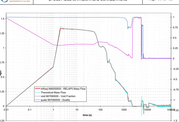
Figure 5.1: Comparison between the RELAP5 and theoretical mass flow, void fraction and quality in DVI SPLIT break line, DVI Test

-0.5 -0.25 0 0.25 0.5 0.75 1 0.01 0.1 1 10 100 1000 10000 100000 time (s) kg /s -1.5 -1.25 -1 -0.75 -0.5 -0.25 0 0.25 0.5 0.75 1

Figure 5.2: Comparison between the RELAP5 and theoretical mass flow, void fraction and quality in ADS Stage-I ST line, DVI Test

(38)

-0.25 0 0.25 0.5 0.75 1 1.25 1.5 1.75 2 2.25 0.01 0.1 1 10 100 1000 10000 100000 time (s) kg /s -1.5 -1.25 -1 -0.75 -0.5 -0.25 0 0.25 0.5 0.75 1 mflowj 143000000 - RELAP5 Mass Flow

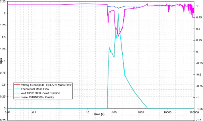
Theoretical Mass Flow void 131010000 - Void Fraction quale 131010000 - Quality

Figure 5.3: Comparison between the RELAP5 and theoretical mass flow, void fraction and quality in ADS Stage-I DT line, DVI Test

-0.5 0 0.5 1 1.5 2 2.5 3 3.5 4 4.5 5 5.5 6 0.01 0.1 1 10 time (s) 100 1000 10000 100000 kg /s -1.5 -1.25 -1 -0.75 -0.5 -0.25 0 0.25 0.5 0.75 1

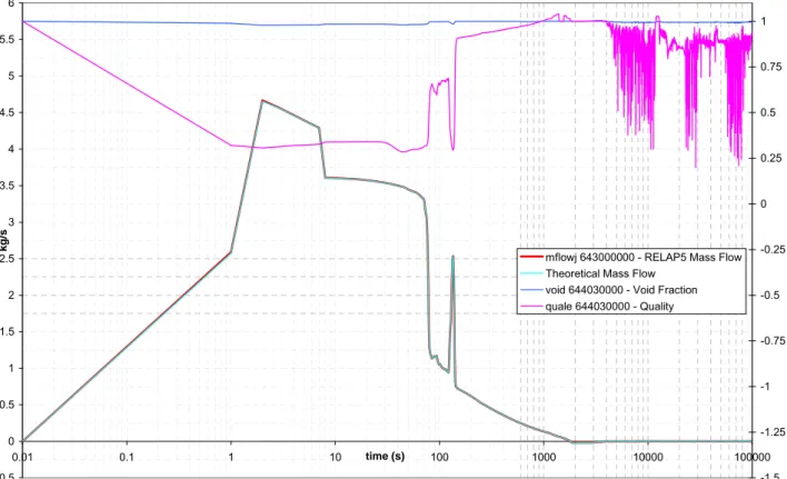
Figure 5.4: Comparison between the RELAP5 and theoretical mass flow, void fraction and quality in EBT SPLIT break line, EBT Test

(39)

-0.2 0 0.2 0.4 0.6 0.8 1 1.2 0.01 0.1 1 10 _{time (s)} 100 1000 10000 100000 kg /s -1.5 -1.25 -1 -0.75 -0.5 -0.25 0 0.25 0.5 0.75 1

Figure 5.5: Comparison between the RELAP5 and theoretical mass flow, void fraction and quality in ADS Stage-I ST line, EBT Test

-0.25 0 0.25 0.5 0.75 1 1.25 1.5 1.75 2 2.25 0.01 0.1 1 10 100 1000 10000 100000 time (s) kg/ s -1.5 -1.25 -1 -0.75 -0.5 -0.25 0 0.25 0.5 0.75 1

Figure 5.6: Comparison between the RELAP5 and theoretical mass flow, void fraction and quality in ADS Stage-I DT line, EBT Test

(40)

-0.5 0.5 1.5 2.5 3.5 4.5 0.01 0.1 1 10 _{time (s)} 100 1000 10000 100000 kg /s -1.5 -1.25 -1 -0.75 -0.5 -0.25 0 0.25 0.5 0.75 1

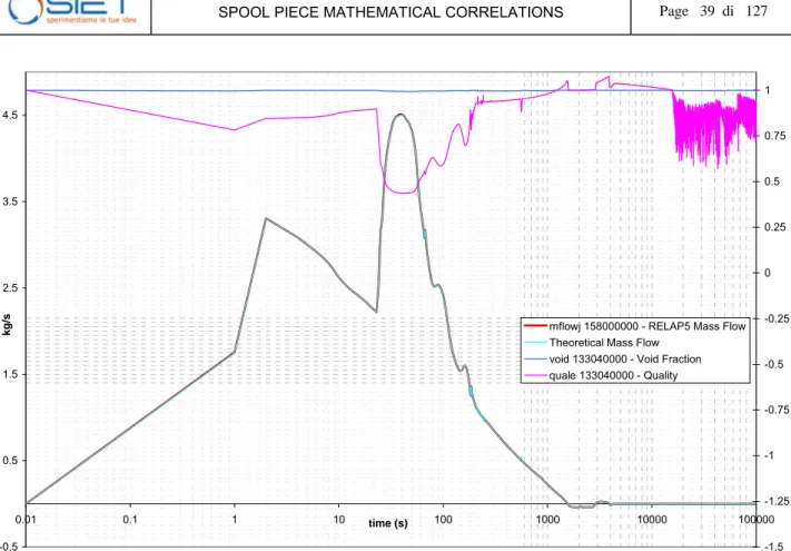
Figure 5.7: Comparison between the RELAP5 and theoretical mass flow, void fraction and quality in ADS SPLIT break line, ADS Test

-0.5 0 0.5 1 1.5 2 2.5 3 3.5 0.01 0.1 1 10 100 1000 10000 100000 time (s) kg/ s -1.5 -1.25 -1 -0.75 -0.5 -0.25 0 0.25 0.5 0.75 1

Figure 5.8: Comparison between the RELAP5 and theoretical mass flow, void fraction and quality in ADS Stage-I DT line, ADS Test

(41)

The Figure 5.9, Figure 5.10, Figure 5.11, Figure 5.12, Figure 5.13, Figure 5.14, Figure 5.15 and Figure 5.16 show the comparison of the calculated and RELAP5 mass flow rates, besides the information on the flow regimes and the presence of choked flow at the rupture orifice (not in the instrumented volume, in which the flow is always not critical). The information about the flow regimes is useful for a correct determination of the Drag Disk shape and for the Turbine Flowmeter models.

The Table 5.1 lists the conventional numbers used in the graph to indicate whether the flow is critical or not and the flow regimes.

Table 5.1: List of the conventional numbers used in the graphs to indicate whether the flow is critical or not and the flow regimes

Choked Flow Flow Regimes

Value Description Value Description

0 Not choked 0.4 Bubbly

1 choked 0.6 Annular Mist

0.7 Mist pre-CHF 1.2 Horizontal stratified -0.25 0 0.25 0.5 0.75 1 1.25 1.5 1.75 2 2.25 2.5 0.01 0.1 1 10 100 1000 10000 100000 time (s) kg /s -2 -1.8 -1.6 -1.4 -1.2 -1 -0.8 -0.6 -0.4 -0.2 0 0.2 0.4 0.6 0.8 1 1.2

floreg 667090000 - Flow Regimes chokef 666000000 - Choked Flow

Figure 5.9: Comparison between the RELAP5 and theoretical mass flow, flow regimes and presence of critical flow in DVI SPLIT beak line, DVI Test

(42)

-0.5 -0.25 0 0.25 0.5 0.75 1 0.01 0.1 1 10 100 1000 10000 100000 time (s) kg/s -2 -1.8 -1.6 -1.4 -1.2 -1 -0.8 -0.6 -0.4 -0.2 0 0.2 0.4 0.6 0.8 1 1.2

Figure 5.10: Comparison between the RELAP5 and theoretical mass flow, flow regimes and presence of critical flow in ADS ST stage I line, DVI Test

-0.25 0 0.25 0.5 0.75 1 1.25 1.5 1.75 2 2.25 0.01 0.1 1 10 100 1000 10000 100000 time (s) kg /s -2 -1.9 -1.8 -1.7 -1.6 -1.5 -1.4 -1.3 -1.2 -1.1 -1 -0.9 -0.8 -0.7 -0.6 -0.5 -0.4 -0.3 -0.2 -0.1 0 0.1 0.2 0.3 0.4 0.5 0.6 0.7 0.8 0.9 1 1.1 1.2 1.3

Figure 5.11: Comparison between the RELAP5 and theoretical mass flow, flow regimes and presence of critical flow in ADS DT stage I line, DVI Test

(43)

-0.5 0 0.5 1 1.5 2 2.5 3 3.5 4 4.5 5 0.01 0.1 1 10 time (s) 100 1000 10000 100000 kg/ s -2.2 -2 -1.8 -1.6 -1.4 -1.2 -1 -0.8 -0.6 -0.4 -0.2 0 0.2 0.4 0.6 0.8 1 1.2

Figure 5.12: Comparison between the RELAP5 and theoretical mass flow, flow regimes and presence of critical flow in EBT SPLIT beak line, EBT Test

-0.2 0 0.2 0.4 0.6 0.8 1 1.2 0.01 0.1 1 10 100 1000 10000 100000 time (s) kg/ s -2 -1.8 -1.6 -1.4 -1.2 -1 -0.8 -0.6 -0.4 -0.2 0 0.2 0.4 0.6 0.8 1 1.2

Figure 5.13: Comparison between the RELAP5 and theoretical mass flow, flow regimes and presence of critical flow in ADS Stage-I ST line, EBT Test

(44)

-0.25 0 0.25 0.5 0.75 1 1.25 1.5 1.75 2 2.25 0.01 0.1 1 10 time (s) 100 1000 10000 100000 kg/ s -2 -1.8 -1.6 -1.4 -1.2 -1 -0.8 -0.6 -0.4 -0.2 0 0.2 0.4 0.6 0.8 1 1.2

Figure 5.14: Comparison between the RELAP5 and theoretical mass flow, flow regimes and presence of critical flow in ADS Stage-I DT line, EBT Test

-0.5 0.5 1.5 2.5 3.5 4.5 0.01 0.1 1 10 time (s) 100 1000 10000 100000 kg /s -2 -1.8 -1.6 -1.4 -1.2 -1 -0.8 -0.6 -0.4 -0.2 0 0.2 0.4 0.6 0.8 1 1.2

Figure 5.15: Comparison between the RELAP5 and theoretical mass flow, flow regimes and presence of critical flow in ADS SPLIT beak line, ADS Test

(45)

-0.5 0 0.5 1 1.5 2 2.5 3 3.5 0.01 0.1 1 10 100 1000 10000 100000 time (s) kg/s -2 -1.8 -1.6 -1.4 -1.2 -1 -0.8 -0.6 -0.4 -0.2 0 0.2 0.4 0.6 0.8 1 1.2

Figure 5.16: Comparison between the RELAP5 and theoretical mass flow, flow regimes and presence of critical flow in ADS Stage-I DT line, ADS Test

Slip ratio, void fraction and quality are related using the standard mass flow rates, as follows:













1 1 1 1 _          L G L G L G L G L L G G G G L G G G V V V V V V V m m m m m x















     _(5.2)





Sx





S

x

L G L G

















1

(5.3)





S



x



x

L G





1

1 





(5.4)







x



x

S

G L





1

1 





, (5.5) in particular,



 



S

x

L G











1

, (5.6)

(46)

Equation (5.6) can be useful to express the mass flow rate (5.1) in another form:











_{  }

_             1 1 1 1 L G L G L L L L G G V V V A V V A m











 (5.7)









_



_



























_





x

V

A

x

V

A

x

V

A

m

_L _L _L _L _L _L

1

1 













. (5.8)

A dimensional analysis shows that it’s possible to determine the mass flow rate from two independent measured variables, according to the following expressions:

 



2



12

V A

m_Void__DD  



_AV 



Drag Disk + Void Fraction Detector (5.9)

 













 T DD T

_V

V

A

m

2





Drag Disk + Turbine Flowmeter (5.10)

T AV T

Void

A

V

m



_









Void Fraction Detector + Turbine Flowmeter (5.11)

As two analytical expressions are enough to solve the equation system, it is possible to use the third expression as checker.

Since the Drag Disk returns the pressure drop in addition to the drag force, two expressions can be derived in order to determine the momentum flux:

 

S D D

A

C

F

V

2



2 

(5.12)

 

K

P

V

2







, (5.13)

It is possible to arrive to 5 different formulations involving the couplings of the three instruments:

Drag Disk + Turbine Flowmeter

 

_              T S D D T C A V F A V V A m 2 1 2



 with Drag Force (5.14)

 

_              T T K V P A V V A m 1 2



Two-phase flow measurement for SPES3 facility: Spool piece mathematical correlations

ENEA

1PN000CA90245

CA90245/1

01 572 RT 09