Casaregola Cosmo
The study of the determination of catalytic properties of Thermal Protection Sys-tem (TPS) materials is carried out at VKI following the Local Heat Transfer Simulation (LHTS) concept developed at the Institute for Problems in Mechan-ics of Moscow (IPM). One of the most important goals of this methodology is to provide a correlation between the external flow conditions and the stagnation point heat flux experienced at the wall. This relation is implicitly provided by means of a boundary layer solver: the VKI Boundary Layer code. The boundary layer calculations needed in the framework of this methodology were originally per-formed under the assumptions of thermal equilibrium and chemical nonequilibrium (CNEQ), i.e. a single temperature describes all the energy modes (translational, rotational, vibrational and electronic one) of the mixture particles.
At this point it is licit to have the curiosity to wonder what will happen if we modify the existing implementation of the code under the different assumption of both thermal and chemical nonequilibrium (TCNEQ)? Which effects will we observe? How will the temperature profiles and the wall heat flux change?
Generally, the modeling of thermal nonequilibrium flows using a multi-temperature approach, could be a very complex task. Hence, in order to simplify this problem, we assume that the plasma is in a state of partial thermal equilibrium. Under this assumption, our two-temperature model can be seen as the most simplis-tic example of thermal nonequilibrum. We assume that all rotational states are fully equilibrated with the translational energies of heavy particles at a common
translational-rotational temperature Thr. In fact, even at ambient temperature,
molecules rotational states are easily excited by collisions with other heavy parti-cles. Moreover, we assume that the translational energies of free electrons, bound
particles, they provoke transitions between bound electronic states. Also, the en-ergies exchange between free and bound electrons and the vibrational states of N2
(the main molecular species in air at standard conditions) is known to be very rapid.
Hence, it will be necessary to explain how the chemistry model will change in the picture and how the energy exchange mechanism, that takes place among particles during collisions and/or chemical reactions, works.
Under the TCNEQ assumption, a new set of governing equations was written and supplemented by a suitable set of boundary conditions; the flow outside the boundary layer is usually considered in Local Thermal Equilibrium (LTE), then the values for velocity, temperatures and mass fractions are fixed by the conditions in the external flow. In agreement with the classical boundary layer hypothesis, the outer edge values are taken from an Euler computation of the external flow. At the wall, we have the no-slip condition for velocity and we assume the
translational-rotational temperature Thr to be equal to the wall temperature while we impose a
zero-derivative for the electro-vibrational one Tev.
In the end, we will compare the results obtained under the assumption of CNEQ and the ones obtained with the modified version in which we have made the assumption of TCNEQ. We will be interested to temperatures, enthalpy and concentrations profiles into the boundary layer along the stagnation line because our final goal is to compute and compare, at the stagnation point, the heat flux obtained in both cases. It worth mentioning that heat flux at the wall is mainly due to two contributions: a thermal conduction one depending on temperature gradient at the wall (in our two-temperature model, we will assume that, at the wall, this contribution is only given by the translational-rotational temperature gradient; in fact, thermal conduction phenomena are mainly due to energy trans-port phenomena by means of heavy particles that collide with the wall) and a minor but not negligible contribution due to the transfer of enthalpy caused by particles diffusion at the wall.
Vorrei ringraziare innanzi tutto le persone che mi hanno dato la possibilit`a di vivere l’interessante esperienza come stagiaire presso il von Karman Institute for Fluid Dynamics: ringrazio il prof. Renzo Lazzeretti ed il prof. Luca d’Agostino per la loro disponbilit`a ed il loro supporto. Sentiti ringraziamenti anche al prof. Mariano Andrenucci ed all’Ing. Salvo Marcuccio che hanno supportato le ultime fasi del mio lavoro.
Un particolare ringraziamento va a tutto il von Karman Institute, al prof. Car-bonaro che non ha esitato nel concedermi la possibilit`a di prendere parte allo stage ed in particolare al prof. Gerard Degrez che dall’alto della sua grande esperienza e del suo inesauribile intuito ha sempre aperto in me nuovi orizzonti e stimolato in-teressanti riflessioni. Inoltre, non potr`o mai dimenticare il fondamentale supporto di Pietro Rini che mi ha spesso permesso di guardare i problemi incontrati con maggiore serenit`a.
Per ultimi, ma solo perch`e i pi`u importanti, i ringraziamenti ai miei genitori ed alle mie sorelle che mi hanno sempre sostenuto in ogni mio passo, ad Eleonora e a tutte quelle persone che con il loro sostegno, hanno reso meno faticosa la strada.
Pisa, Italia Cosmo Casaregola
I would like to thank all the people that gave me the opportunity to live such an interesting experience as stagiaire in von Karman Institute for Fluid Dynamics: special thanks to prof. Renzo Lazzeretti and prof. Luca d’Agostino for their availability and support. Thanks to prof. Mariano Andrenucci and Ing. Salvo Marcuccio for their support in the final part of my work.
Special thanks to all the von Karman Institute, to prof. Mario Carbonaro who never hesitated to let me join the VKI. In particular I would like to thank prof. Gerard Degrez because he has surprised me day by day with his great experience, intuition and original suggestions and Pietro Rini: I will never forget your fundamental support that often helped me even in the worst moments and in my eyes this is what makes you a great advisor.
Finally, but surely the most important, special thanks to my parents and to my sisters for their continuous spiritual support, thanks to Eleonora for the warmth she gives me and to all those people who never hesitated to make this hard task softer.
Pisa, Italy Cosmo Casaregola
Abstract i
Ringraziamenti iii
Acknowledgements v
Table of Contents vii
List of Symbols ix
1 Introduction 1
1.1 Aerothermochemistry phenomenology . . . . 1
1.2 Applications . . . 3
1.3 Thesis background . . . 6
1.3.1 TPS properties determination metodology . . . 7
1.4 Thesis outline and aim of the project . . . 9
1.5 Contents of this research . . . 10
2 Mixture properties 13 2.1 Introduction . . . 13 2.2 Thermodynamic properties . . . 13 2.3 Chemistry . . . 15 2.3.1 Vibrational Nonequilibrium . . . 16 2.3.2 Chemical Nonequilibrium . . . 19 2.3.3 Arrhenius Law . . . 20
2.3.4 Chemical mass production term . . . 23
2.4 Nonequilibrium, Equilibrium and Frozen Flows . . . 24
2.5 Transport properties . . . 25
2.5.1 Molecular description . . . 26
2.5.2 Transport fluxes definition . . . 27
2.5.3 Particles with internal degrees of freedom: the Eucken cor-rection . . . 28
2.5.4 Boltzmann equation . . . 29
2.5.6 Heavy particles transport properties . . . 32
2.5.7 Electron transport properties . . . 33
2.5.8 Diffusion in two temperature plasmas . . . 34
2.6 Heterogeneous Catalycity . . . 36
2.6.1 Catalytic wall model implementation . . . 39
3 Nonequilibrium Boundary Layer 43 3.1 Introduction . . . 43
3.2 Two-temperature model assumption . . . 43
3.3 Multi-temperature chemistry modeling and energy exchanges . . . . 44
3.3.1 Park’s multi-temperature approach . . . 44
3.3.2 Electro-vibrational energy loss due to chemistry . . . 45
3.3.3 Energy exchange terms . . . 46
3.4 Governing Equations . . . 48
3.4.1 Equation of state . . . 48
3.4.2 Continuity equation . . . 48
3.4.3 Species continuity equation . . . 48
3.4.4 Momentum equation . . . 49
3.4.5 Energy equations . . . 50
3.4.6 Boundary layer equations . . . 52
3.4.7 Boundary conditions . . . 53
3.4.8 Enthalpy-Temperature relationship . . . 54
3.4.9 Lees-Dorodnitsyn transformation . . . 55
3.4.10 Transformed boundary layer equations at the stagnation line 58 4 Numerical methods 61 4.1 Introduction . . . 61
4.2 Numerical solution of the boundary layer governing equations . . . 61
4.2.1 Discretization in ξ-direction . . . 62
4.2.2 Hermitian discretization in η direction . . . 63
4.3 Thomas algorithm for linear tridiagonal systems . . . 66
4.4 Diffusion fluxes computation . . . 70
5 Results 73 5.1 Boundary Layer Computations . . . 73
5.1.1 Boundary conditions and wall reactions . . . 75
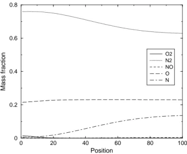
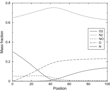
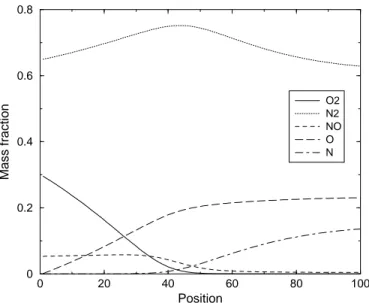
5.1.2 5-species Air mixture . . . 76
5.1.3 7-species Air mixture . . . 90
5.1.4 Effectiveness of the BL code under the assumption of TCNEQ107 5.1.5 Heat flux comparison . . . 109 6 Conclusions and further research 111
B The Lees-Dorodnitsyn transformation in axisymmetric geometry115
Superscripts
(·)? refers to equilibrium conditions
Subscripts
(·)b refers to the backward reaction
(·)f refers to the forward reaction
(·)e refers to the boundary layer outer edge
(·)w refers to the wall
Greek symbols
ηf second coefficient of Arrhenius law
Θf first coefficient of Arrhenius law
χk rate of reaction of the kth surface per unit time
ξ Lees-Dorodnitsyn non dimensional tangent coordinate
ξj number of atom grams of element j per unit volume
δ non dimensional boundary layer thickness
ρ density
²0 energy threshold
ˆ
η Lees-Dorodnitsyn non dimensional normal coordinate
γi recombination probability of ith species
λij number of elements j per molecule of species i
˙
Wi mass production term due to chemical reaction
˙
Wi,cat mass production term due to catalytic surface reactions
ν00
i stoichiometric coefficient for the ith species thought as a product
ν0
Alphanumeric symbols
Cf first coefficient of Arrhenius law
kb backward reaction rate
M catalytic species
~
Ji diffusion flux for the ith species
g non dimensional enthalpy
he outer edge enthalpy
y physical normal coordinate (m)
Kc equilibrium constant for the reaction
kf forward reaction rate
x physical tangent coordinate (m)
yi mass fraction
Mi molar mass of the ith species
Nspec, Ns number of species
nel number of elements
Ni number of moles of the ith species
r local radius of the probe
Cp specific heat at constant pressure (J/kg K)
Te outer edge temperature
Tw wall temperature
Xs any chemical species
[Xs] concentration of the sth chemical species
~
V mass averaged mixture velocity
~
Vi velocity of ith species
~
Ui diffusion velocity of ith species
˜
3.1 Overview of reactions and chosen rate-controlling temperatures in the chemical-kinetics model of Dunn and Kang . . . 45 4.1 Coefficients for the hermitian discretization of the boundary layer
equations . . . 65 5.1 Reaction rate coefficients for Earth Atmosphere (Air 57 species)
-Dissociation reactions . . . 74 5.2 Reaction rate coefficients for Earth Atmosphere (Air 5 species)
-Bimolecular exchange . . . 75 5.3 Reaction rate coefficients for Earth Atmosphere (Air 7 species) -
Bi-molecular exchange (1st and 2nd), associative ionization-dissociative
recombination (3rd) and heavy particle impact ionizations (4th,5th
and 6th) . . . 75
5.4 Test cases for 5-species and 7-species air mixture . . . 75 5.5 Test cases for the computation of the wall heat flux . . . 109
1.1 Capsule re-entering the Earth’s atmosphere (courtesy Aerospatiale) 4 1.2 Heat flux probe in the exhaust jet of the VKI plasmatron wind tunnel 5
1.3 VKI mini-torch in operation . . . 6
1.4 TPS catalytic properties determination . . . 8
2.1 Molecules’ energy modes . . . 15
2.2 Fully catalytic wall . . . 36
2.3 Partially catalytic wall . . . 37
2.4 Non catalytic wall . . . 37
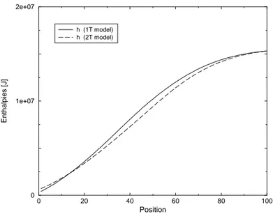
5.1 Enthalpy profiles in case of 5-species Air mixture - Non catalytic wall- Test Case 1 . . . 76
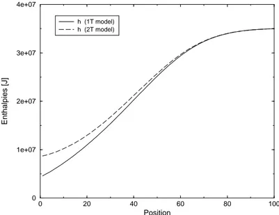
5.2 Enthalpy profiles in case of 5-species Air mixture - Fully catalytic wall- Test Case 1 . . . 77
5.3 Enthalpy profiles in case of 5-species Air mixture - Non catalytic wall- Test Case 2 . . . 78
5.4 Enthalpy profiles in case of 5-species Air mixture - Fully catalytic wall- Test Case 2 . . . 79
5.5 Enthalpy profiles in case of 5-species Air mixture - Non catalytic wall- Test Case 3 . . . 79
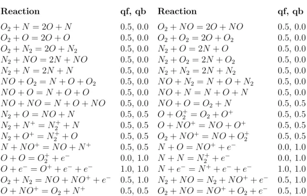
5.6 Enthalpy profiles in case of 5-species Air mixture - Non catalytic wall- Test Case 4 . . . 80
5.7 Temperature profiles in case of 5-species Air mixture - Non catalytic wall- Test Case 1 . . . 80
5.8 Temperature profiles in case of 5-species Air mixture -Fully catalytic wall- Test Case 1 . . . 81
5.9 Temperature profiles in case of 5-species Air mixture - Non catalytic wall- Test Case 2 . . . 82
5.10 Temperature profiles in case of 5-species Air mixture -Fully catalytic wall- Test Case 2 . . . 82 5.11 Temperature profiles in case of 5-species Air mixture - Non catalytic
wall- Test Case 3 . . . 83 5.12 Temperature profiles in case of 5-species Air mixture - Non catalytic
wall- Test Case 4 . . . 83 5.13 Concentrations profiles in case of 5-species Air mixture - Non
cat-alytic wall- CNEQ- Test Case 1 . . . 84 5.14 Concentrations profiles in case of 5-species Air mixture - Non
cat-alytic wall- TCNEQ- Test Case 1 . . . 85 5.15 Concentrations profiles in case of 5-species Air mixture - Fully
cat-alytic wall- CNEQ- Test Case 1 . . . 85 5.16 Concentrations profiles in case of 5-species Air mixture - Fully
cat-alytic wall- TCNEQ- Test Case 1 . . . 86 5.17 Concentrations profiles in case of 5-species Air mixture - Non
cat-alytic wall- CNEQ- Test Case 2 . . . 86 5.18 Concentrations profiles in case of 5-species Air mixture - Non
cat-alytic wall- TCNEQ- Test Case 2 . . . 87 5.19 Concentrations profiles in case of 5-species Air mixture - Fully
cat-alytic wall- CNEQ- Test Case 2 . . . 87 5.20 Concentrations profiles in case of 5-species Air mixture - Fully
cat-alytic wall- TCNEQ- Test Case 2 . . . 88 5.21 Concentrations profiles in case of 5-species Air mixture - Non
cat-alytic wall- CNEQ- Test Case 3 . . . 88 5.22 Concentrations profiles in case of 5-species Air mixture - Non
cat-alytic wall- TCNEQ- Test Case 3 . . . 89 5.23 Concentrations profiles in case of 5-species Air mixture - Non
cat-alytic wall- CNEQ- Test Case 4 . . . 89 5.24 Concentrations profiles in case of 5-species Air mixture - Non
cat-alytic wall- TCNEQ- Test Case 4 . . . 90 5.25 Enthalpy profiles in case of 7-species Air mixture - Non catalytic
wall- Test Case 1 . . . 91 5.26 Enthalpy profiles in case of 7-species Air mixture - Fully catalytic
wall- Test Case 1 . . . 91 5.27 Enthalpy profiles in case of 7-species Air mixture - Non catalytic
5.28 Enthalpy profiles in case of 7-species Air mixture - Fully catalytic wall- Test Case 2 . . . 92 5.29 Enthalpy profiles in case of 7-species Air mixture - Non catalytic
wall- Test Case 3 . . . 93 5.30 Enthalpy profiles in case of 7-species Air mixture - Fully catalytic
wall- Test Case 3 . . . 93 5.31 Enthalpy profiles in case of 7-species Air mixture - Non catalytic
wall- Test Case 4 . . . 94 5.32 Enthalpy profiles in case of 7-species Air mixture - Fully catalytic
wall- Test Case 4 . . . 94 5.33 Temperature profiles in case of 7-species Air mixture - Non catalytic
wall- Test Case 1 . . . 95 5.34 Temperature profiles in case of 7-species Air mixture -Fully catalytic
wall- Test Case 1 . . . 95 5.35 Temperature profiles in case of 7-species Air mixture - Non catalytic
wall- Test Case 2 . . . 96 5.36 Temperature profiles in case of 7-species Air mixture -Fully catalytic
wall- Test Case 2 . . . 96 5.37 Temperature profiles in case of 7-species Air mixture - Non catalytic
wall- Test Case 3 . . . 97 5.38 Temperature profiles in case of 7-species Air mixture - Fully
cat-alytic wall- Test Case 3 . . . 97 5.39 Temperature profiles in case of 7-species Air mixture - Non catalytic
wall- Test Case 4 . . . 98 5.40 Temperature profiles in case of 7-species Air mixture - Fully
cat-alytic wall- Test Case 4 . . . 98 5.41 Concentrations profiles in case of 7-species Air mixture - Non
cat-alytic wall- CNEQ- Test Case 1 . . . 99 5.42 Concentrations profiles in case of 7-species Air mixture - Non
cat-alytic wall- TCNEQ- Test Case 1 . . . 100 5.43 Concentrations profiles in case of 7-species Air mixture - Fully
cat-alytic wall- CNEQ- Test Case 1 . . . 100 5.44 Concentrations profiles in case of 7-species Air mixture - Fully
cat-alytic wall- TCNEQ- Test Case 1 . . . 101 5.45 Concentrations profiles in case of 7-species Air mixture - Non
5.46 Concentrations profiles in case of 7-species Air mixture - Non cat-alytic wall- TCNEQ- Test Case 2 . . . 102 5.47 Concentrations profiles in case of 7-species Air mixture - Fully
cat-alytic wall- CNEQ- Test Case 2 . . . 102 5.48 Concentrations profiles in case of 7-species Air mixture - Fully
cat-alytic wall- TCNEQ- Test Case 2 . . . 103 5.49 Concentrations profiles in case of 7-species Air mixture - Non
cat-alytic wall- CNEQ- Test Case 3 . . . 103 5.50 Concentrations profiles in case of 7-species Air mixture - Non
cat-alytic wall- TCNEQ- Test Case 3 . . . 104 5.51 Concentrations profiles in case of 7-species Air mixture - Fully
cat-alytic wall- CNEQ- Test Case 3 . . . 104 5.52 Concentrations profiles in case of 7-species Air mixture - Fully
cat-alytic wall- TCNEQ- Test Case 3 . . . 105 5.53 Concentrations profiles in case of 7-species Air mixture - Non
cat-alytic wall- CNEQ- Test Case 4 . . . 105 5.54 Concentrations profiles in case of 7-species Air mixture - Non
cat-alytic wall- TCNEQ- Test Case 4 . . . 106 5.55 Concentrations profiles in case of 7-species Air mixture - Fully
cat-alytic wall- CNEQ- Test Case 4 . . . 106 5.56 Concentrations profiles in case of 7-species Air mixture - Fully
cat-alytic wall- TCNEQ- Test Case 4 . . . 107 5.57 Variation of electro-vibrational temperature profile with respect to
the elastic relaxation time τeh . . . 108
5.58 Variation of translational-rotational temperature profile with re-spect to the elastic relaxation time τeh . . . 108
5.59 TCNEQ boundary layer wall heat flux compared to CNEQ bound-ary layer wall heat flux for a 5-species Air mixture - Abacus 1 . . . 109 5.60 TCNEQ boundary layer wall heat flux compared to CNEQ
bound-ary layer wall heat flux for a 7-species Air mixture - Abacus 1 . . . 110 5.61 TCNEQ boundary layer wall heat flux compared to CNEQ
Introduction
“The entity of experimental knowledge and theories involving physical chemistry,
in addition to fluid mechanics and thermodynamics” [34].
With this sentence, Th. von K´arm´an defined the ”Aerothermochemistry” as the overall phenomena described by aerothermodynamics that requires contributions from fluid dynamics, thermodynamics, statistical mechanics, quantum theory, ki-netic theory, chemistry.
All these different contributions have to be taken together in a self consistent way; the hypothesis made on the modeling of a constitutive term of the governing equa-tions have to be consistent with the ones made in the modeling of a different, but somewhat interacting term.
The present numerical research activity is involved in the design of Thermal Pro-tection System ( TPS ) for space vehicle and would have just the goal to be a little contribute in such a huge and amazing topic.
In the following, we will briefly summarize the aerothermochemistry phenomenol-ogy and some of the typical applications of this discipline.
1.1
Aerothermochemistry phenomenology
It is well known that a fluid, in the most general case, is made of a mixture of atoms and molecules. Air at ambient temperature, for example, is a mixture made of molecular nitrogen, molecular oxygen, argon, carbon dioxide, neon, plus some other minor components. At moderate temperatures the gas behaves, with good approximation, as a calorically perfect gas. Gas pressure (p), density (ρ) and tem-perature (T ) are linked by the well known and simple state law: p = ρRT (where
R is the so called perfect gas specific constant). The gas specific heats are constant
When temperature rises, this simple picture non longer exists: new phenom-ena, that will be called high temperature effects, appear and the gas nature is dramatically changed. The principal high temperature effects may be summarized as follows.
• As temperature rises, the internal energy modes of the gas atoms and molecules,
that at room temperature are dormant, are excited. Specific heats become a function of temperature and internal energy and enthalpy are now non-linear functions of the temperature. The specific heats ratio, also called
γ, is no longer a constant. For air excitation of the internal energy modes
(vibrational) becomes important above temperatures of 500-800 K.
• As temperature further rises, chemical reactions can occur. Molecules
disso-ciate into atoms, new molecules are eventually formed, atoms and molecules can ionize. Mixture internal energy and enthalpy become functions not only of temperature but also of the chemical composition.
• Thermal nonequilibrium can also occur: internal energy modes are out of
equilibrium with respect to the translational one. For example, when a fluid element crosses a shock, the translational energy of the fluid particles is suddenly increased. It is well known [1, 28], that a high number of collisions is needed to equilibrate the internal energy modes with the translational one. Therefore, behind the shock, there will be a relaxation region where the internal energy modes will try to “catch up” the translational one. Another example is when the fluid experiences a strong expansion. In this case the translational energy will rapidly decrease because of the expansion, but the internal one will remain higher. When the mixture is ionized, an additional source of thermal nonequilibrium appears because energy exchange between mixture components and free electrons is highly inefficient due to the large mass disparity: in this case the translational temperature of electrons can be different from the one of heavy particles [28].
• If the temperature is high enough, ionization can occur and the gas becomes
a partially ionized plasma, with a finite electrical conductivity. Therefore electromagnetic fields and associated forces, either self-induced or applied from an external source [30, 37] can act on the fluid, appreciably changing its behaviour with respect to a neutral one.
• At high temperature (above 10000-11000 K for air) radiation emitted and
distribution in the flowfield. Radiation modeling is a formidable task [28, 35, 40], both numerically (a fluid element, a priori, is influenced by and influences all the others) and physically and will not be attempted in this thesis.
• Chemical reactions can take place not only in the bulk of the gas but also
at the surface of the vehicle due to catalytic effects of the wall material upon surface chemistry. Usually such reactions have the negative property of increasing the heat flux experienced by the vehicle [26, 35].
1.2
Applications
In the following, we will briefly present some practical cases in which most of the effects described in sec. 1.1 are encountered.
Re-entry vehicles
When an aerospace vehicle, as for example the Space Shuttle or the Soyuz capsule, enters the upper layers of a planetary atmosphere from space, it develops very high velocities. As denser, lower atmospheric layers are reached, the spacecraft loses its kinetic energy through collisions with molecules and atoms in the atmosphere. On a macroscopic point of view, this gives rise to a strong, hypersonic bow shock in front of the vehicle. Behind the shock, density dramatically increases and tem-peratures rise to several thousands Kelvin degrees (Fig. 1.1).
Hence, a major part of the kinetic energy of the free stream flow is converted into thermal energy across the shock and therefore high temperature is reached in the flow region between the shock and the body (the shock layer), especially around the body nose, where the shock reaches its maximum intensity. That is why, to prevent any damage to the spacecraft, its windward side needs to be protected by a heat shield made of advanced thermal protection materials.
Downstream of the nose region the gas expands and reaches again a high Mach number: the intense friction happening in the boundary layer increases its tem-perature triggering further chemical reactions. If temtem-perature in the shock layer is high enough the gas can ionize: the free electrons that are created absorb radio waves and cause communication blackout to and from the vehicle. This is a serious problem and an accurate prediction of the electrons number density in the shock layer is important. Emission and absorption of radiation can occur and, besides affecting the state of the gas surrounding the vehicle, can raise the heat flux ex-perienced by the vehicle itself. Radiation from the hot vehicle wall to the ambient
Figure 1.1: Capsule re-entering the Earth’s atmosphere (courtesy Aerospatiale)
atmosphere can have a significant cooling effect and must be taken into account in the thermal boundary condition [35].
High enthalpy wind tunnels
Conventional hypersonic wind tunnels are not able to simulate nonequilibrium flows over bodies, because the maximum attainable temperature is not enough to trigger high temperature effects. Facilities that can provide the needed tem-perature level in a continuous way (testing time of the order of minutes) are arc heaters [23] and inductively coupled plasma (ICP) heaters [6].
In arc heaters the testing gas is heated to high temperature by an electric arc discharge in the reservoir and then the chemically reacting mixture expands through a hypersonic nozzle in the test section where the model is located. In this kind of facility flow temperature are both high, approaching real flight conditions. A main drawback of arc heaters is that the copper electrodes (used to generate the electric arc) are progressively eroded and the gas is contaminated by metal va-por. The metal vapor is deposited on the testing model and changes its catalytic properties: this effect is particularly adverse when aging tests on the model mate-rial are conducted. Although the pollution levels are very low in state-of-the-art
arc heaters (copper fraction as low as 1 PPM), many researchers, especially from Russia, prefer to use ICP heaters.
In a ICP heater such as the VKI plasmatron (Fig. 1.2) and the VKI mini-torch (Fig. 1.3) the plasma is generated by electromagnetic induction: a coil, traversed by a high frequency, high voltage current, surrounds a quartz tube in which cold gas is injected. Induced electromagnetic oscillating fields exist inside the quartz tube.
Figure 1.2: Heat flux probe in the exhaust jet of the VKI plasmatron wind tunnel These fields move the free electrons present in the gas and create currents that heat the gas by Joule effect. The heated gas dissociates and ionizes into a plasma. These facilities show no pollution of the gas because there is no direct contact with the coils and the testing time can be, at least in theory, indefinitely long. Usually these facilities operate at low Mach number regime, even if they can be suitably adapted to produce supersonic flow [12].
Ramjet and Scramjet engines
A Ramjet engine is essentially a duct where supersonic air is slowed down to sub-sonic speed at the entrance of the combustor. Fuel is injected in the combustor,
Figure 1.3: VKI mini-torch in operation
the mixture burns and expands through the nozzle. Ramjets have advantages over conventional turbine engines in the Mach number regime from 2 to 5. However, some design concepts of hypersonic airbreathing transport vehicles assume a flight Mach number well in excess of 10. Under such conditions, if the incoming air is decelerated to subsonic speed, it attains a temperature that is above the adiabatic flame temperature of the fuel-air burning process in the combustor and therefore no combustion can take place. A possible solution is to keep the incoming air stream at supersonic speed in the combustor: in this way air temperature is kept below the flame adiabatic temperature and combustion can take place. The ma-jor drawback is that the combustion has to take place in a supersonic stream, leading to tremendous practical problems (flame stabilization, efficient mixing and burning) that are still not solved nowadays.
1.3
Thesis background
The present research activity is involved in the determination of the heat flux flowing through the surface of atmospheric re-entry vehicles. This complex task carried out at von Karman Institute can be accomplished by means of both nu-merical code and experimental facilities. In the following a brief description of the metodology is presented.
1.3.1
TPS properties determination metodology
The design of Thermal Protection Systems (TPS) materials for space (re-)entry vehicles requires to know as accurately as possible the catalytic properties of the TPS materials. Indeed, for a given wall temperature and free stream properties (total enthalpy, pressure and velocity), the wall heat flux will depend strongly on the wall catalytic activity if the boundary layer developing on it is far from chemical equilibrium. For example, the stagnation point heat flux can differ by a factor larger than two between a non-catalytic and a fully catalytic surface.
While, until recently, the design calculations have been done assuming the most unfavorable conditions (i.e. a fully catalytic wall), the design of next-generation reusable space vehicles needs a better estimation of the finite rate catalysis of the TPS materials, in order to reduce weight and operative costs of long-range missions such as Mars exploration.
This was the motivation for the construction at VKI of a large scale ICP facility (Plasmatron). Since a TPS catalytic activity cannot be measured directly, a metodology has been developed in order to deduce the catalytic properties of TPS materials from their effect on the wall heat flux. This metodology, schematically represented in Fig. 1.4, is composed of the following blocks:
1. A LTE (Local Thermal Equilibrium) viscous flow simulation of the flow in the ICP facility heating chamber and in the downstream subsonic plasma jet. For given fluid and inlet flow swirl angle, the flow in an ICP facility depends on three operational parameters: the inlet mass flow, the pressure level and the power injected in the plasma. In LTE flow however, it has been shown that the flow pattern depends almost exclusively on the inlet mass flow, which controls directly the Reynolds number. The purpose of the LTE viscous flow simulation is therefore to compute the values of the non-dimensional parameters Πi which characterize the flow near the stagnation
point of the heat flux probe.
2. Experimental measurements of the stagnation point wall heat flux (qw) and the Pitot pressure (∆p) on a cold wall (Tw ∼= 300 K) reference heat flux
probe assumed to be fully catalytic.
3. Reconstruction of the plasma jet enthalpy and velocity gradient at the edge of the stagnation point boundary layer using the measured stagnation point heat flux and Pitot pressure. Boundary layer analysis reveals that the stag-nation point heat flux to the catalytic probe wall depends on the following parameters:
Figure 1.4: TPS catalytic properties determination
• the thermodynamic state at the boundary layer edge, which, assuming
chemical equilibrium of the incoming flow, is completely determined by
pe and he
• the radial velocity gradient (∂v
∂r) at the boundary layer edge
• the boundary layer thickness (δ) and the product ue∂x∂
¡∂v
∂x
¢
e (needed
since finite boundary layer effects are taken into account)
• the wall catalytic activity represented by a unique recombination
prob-ability γw and the wall temperature Tw
Among these parameters, only two (heand ∂v∂r) are unknown: the stagnation
pressure and wall temperature are known experimentally, the recombination probability γw is equal to one according to the hypothesis of fully catalytic
wall, the boundary layer thickness and ue∂x∂
¡∂v
∂x
¢
e are related to the velocity
gradient and to the probe radius R through the non-dimensional hydrody-namic parameters Πi. So one finally can write:
qw = BL(he,
∂v
in which only the two first parameters are unknown. Besides, the pitot pressure, the outer edge density ρe and the radial velocity gradient at the
boundary layer edge ∂v
∂r are linked together through a third non-dimensional
hydrodynamic parameter obtained from the LTE viscous flow simulation, i.e.
∆p = Π3ρe(pe, he) µ R µ ∂v ∂r ¶ e ¶2 (1.3.2)
Provided that the functional form 1.3.1 is known (it is implicitly provided by running a nonequilibrium boundary layer solver), the two unknown flow quantities can be determined by solving the system 1.3.1- 1.3.2 by some suitable iterative scheme.
4. Calculation of heat flux abacus. Once the plasma enthalpy and velocity gra-dient at the boundary layer edge have been determined, the boundary layer solver can be run for various wall catalytic-activity/temperature combina-tion to produce a heat flux abacus (i.e. a set of qw-Tw curves at constant
catalytic activity γw).
5. Experimental measurement of the stagnation point heat flux to a TPS ma-terial sample and of its temperature, and determination of the mama-terial cat-alytic activity. This can be done graphically using the heat flux abacus by identifying the contour on which the data point (qw,Tw) lies.
1.4
Thesis outline and aim of the project
Different numerical codes have been developed at VKI in order to study and char-acterize the behaviour of high enthalpy reacting flows.
During my stage in VKI, I had the opportunity to use the VKI Boundary Layer
code [2], that is a finite difference 2-D/axisymmetric solver for a boundary layer,
also suitable for the description of the flow field in the stagnation region of a low Reynolds number flow. In the present work the code have been used in this second way, in order to evaluate the flow properties around the stagnation line.
One of the main strengths of the code is the flow characterization from a phys-ical and chemphys-ical point of view; indeed, state-of-the-art physphys-ical and chemphys-ical theories have been applied by means of a library for the perfect gases also devel-oped at the von Karman Institute. This library, named PEGASE (PErfect GAS
Equation solver), [3], can be used both as a stand-alone program and as an
exter-nal library to support a CFD code. In the present work PEGASE have been used in both ways.
Moreover, the PEGASE libraries allow users to define also mixtures that are in thermal nonequilibrium; in this work, we have often called PEGASE libraries from the VKI BL code in this way. In fact, the VKI BL code [2] was implemented under the assumption of thermal equilibrium and chemical nonequilibrium (CNEQ), in which a single temperature describes all the energy modes (translational, rota-tional, vibrational and electronic one) of the mixture particles.
The aim of this project is to modify the existing implementation introducing a multi-temperature model in order to analyze the influence of thermo-chemical nonequilibrium (TCNEQ) along the stagnation line flows.
Besides, in order to simplify the modeling of TCNEQ, in the new model the plasma will be considered in a state of partial thermal equilibrium: a
translational-rotational temperature (Thr) will describe the translational and rotational energy
modes and an electro-vibrational temperature (Tev) the vibrational and electronic
ones.
From a practical point of view, in the modified implementation, all the routines and coefficients depending on a single-temperature will be modified. In fact, since our mixture will be described by two temperatures, the energy equation will be replaced by two-coupled equations respectively for the Total and the Electro-Vibrational energies.
1.5
Contents of this research
The theoretical background related to the subject has been summarized in chapter 2, where the physical meaning of thermochemical nonequilibrium is discussed, as far as its field of application is concerned. Moreover, in this section, the last part is dedicated to the explanation of the wall catalycity effects.
Chapter 3 is dedicated to the explanation of the two-temperature plasma flow assumption; besides we will outline the governing equations of our problem and their coordinate transformation in order to obtain a self-similar boundary layer.
In Chapter 4 the numerical methods used to obtain the results achieved in this work are presented. The procedure used have been taken from the original implementation done by P.F.Barbante [2].
In Chapter 5 the computations and the results obtained for a TCNEQ bound-ary layer are presented and compared to the CNEQ case. We have focused our attention on two kinds of air mixture, a 5-species and a 7-species one, in four test cases in order to analyze enthalpy, temperature and species concentration profiles. In the end we have compared the wall heat flux obtained in TCNEQ and CNEQ model.
Finally in Chapter 6 some conclusions and suggestions for further improve-ments about this subject are presented.
Mixture properties
2.1
Introduction
In this chapter we will focus our attention to both equilibrium and nonequilibrium properties of a chemical reacting mixture.
High temperature fluids are generally made of different species and each one, in the range of pressure and temperature of interest here, behaves with good ap-proximation as a perfect gas. We assume also that the gas can be described as a continuum: the macroscopic properties may be identified with average values of the appropriate molecular quantities at any location in the flow. This identi-fication is valid as long as there are a sufficient number of molecules within the smallest significant volume of the flow.
In order to better understand the physical-chemical models that are used to de-scribe the flows studied in this research, we will outline the thermodynamic prop-erties, the chemistry and the transport properties of our mixture.
Moreover we will have a look at the important catalytic processes that take place near the solid surface.
2.2
Thermodynamic properties
In the most general case, we could think plasma flows are composed of monoatomic particles (neutral atoms or atomic ions), polyatomic particles (neutral molecules or molecular ions) and free electrons. Moreover we can group monoatomic and polyatomic particles under the name of heavy particles.
Quantum physics shows that atoms and molecules have different modes to store energy and that each mode is quantized (see [1, 40]), i.e. it can only take discrete values. We have:
• Translational energy mode (eth): associated with the motion of centre of mass
eth,s =
3
2RsTs (2.2.1)
where Rs is the specific gas constant of species s and Ts its temperature.
• Rotational energy mode (erot): associated with the rotation of the molecule
around three orthogonal axes in space. In the hypothesis of diatomic molecules behaving as rigid rotator- harmonic oscillator
erot,s = RsTs µ 1 − θR θR+ 3Ts ¶ (2.2.2)
where θR is the rotational characteristic temperature.
• Vibrational energy mode (evib): associated with the vibration of the atoms
of the molecule with respect to equilibrium positions within the molecule. In the same hypothesis of the previous point
evib,s= Rs
θV
eθVTs − 1
(2.2.3)
where θV is the vibrational characteristic temperature.
• Electronic energy mode (eel): associated with the electrons orbiting around
the nucleus eel,s = Rs ∞ P k=0 gkθE,kexp ³ −θE,k Ts ´ ∞ P k=0 gkexp ³ −θE,k Ts ´ (2.2.4)
where gk is the degeneracy for level k, θE,k is the characteristic electronic
temperature for level k. The series diverges and has to be truncated.
With respect to the previous classification, we can write:
• Atoms: they have only the translational and electronic energy mode; • Polyatomic particles (molecules): they have all the energy modes;
Figure 2.1: Molecules’ energy modes
• Free electrons: they have only the translational mode;
At this point, it is useful to introduce a specification; rotational, vibrational and electronic states are said to be the internal degrees of freedom and they are coupled together. Actually, (see [3], [5]), coupling effects start to play an important role at very high temperatures for which molecules rotate and vibrate so strongly that most of them have dissociated anyway. Hence, we may neglect coupling effects and simplify our model considering internal degrees separately.
Moreover we can define various macroscopic properties of our mixture (see [39]):
• the species mass density ρs = nsmswhere ns is the number density of species
s or the number of s-particles per unit volume and ms is the mass of a single
particle of species s; the mixture number density is n = Psns and the
mixture mass density is ρ =Psρs
• about chemical composition we have the mole fractions xs = ns/n and the
mass fractions ys = ρs/ρ
• we may define the partial pressure ps = nskBTs where kB is the Boltzmann
constant and the mixture pressure is given by p =Psps
• the species internal energies per unit mass es = eth−s+erot−s+evib−s+eel−s+
ech−swhere ech−sis the species formation energy (per unit mass, at 0 K) and
2.3
Chemistry
In this section we will deal with vibrational and chemical processes. They all take place by molecular collisions and/or radiative interactions but, in this work, we will neglect the radiative interactions; then chemical and vibrational changes will take place only due to collisions that, depending on collision frequency, will take time to occur.
We can consider a fluid dynamic system in equilibrium when gas has enough time for the necessary collisions to occur without changing is properties at a fixed pressure and temperature conditions independent of time.
On the other hand, in high-speed gas dynamics the gas is not always given the luxury of the necessary time to reach the equilibrium. Indeed, each fluid element will need some time (i.e. a certain number of collisions) to approach the equilibrium conditions, and, by the time enough collisions have occurred, the fluid elements has moved a certain distance downstream, where there are different values of pressure and temperature.
2.3.1
Vibrational Nonequilibrium
As we have said before, molecules and atoms have several modes to store energy. They both have translational and electronic energy, while only molecules have the rotational and vibrational one.
According to quantum mechanics, each of the energetic modes described in sec. 2.2, is quantized, i.e. they can exist only at certain discrete values.
Let us consider [1, 40] a generic molecule with a certain vibrational energy level diagram, and let us focus our attention on the ith level. The population of this
level, Ni, will be increased from particles coming from the i − 1th and i + 1th levels,
and decreased from the particles jumping from the ith level up to i + 1th or down
to i − 1th levels.
Let Pi+1,i be the ”transition probability” i.e. the probability that a molecule
in the ith level, upon collision with another molecule, will jump up to the i + 1th
level. Physically it can be interpreted on a dimensional basis as the number of transitions per collision per particles.
Let Z be the collision frequency then the number of collisions per particle per second.
Let ki+1,i be the product of the collision frequency Z with the probability Pi+1,i,
then it represents the number of transitions per particle per second, one obtains, for the net rate of change of the population in the ithlevel, the ”master equation
for vibrational relaxation”: dNi
dt = ki+1,iNi+1,i+ ki−1,iNi−1,i− ki,i+1Ni,i+1− ki,i−1Ni,i−1 (2.3.1)
In particular, when the system is in equilibrium, we will have dNi
dt = 0, then each
transition in a given direction is exactly balanced by its counterpart in the opposite direction so that the net interchange between any two adjacent states must be zero. This is the so called ”principle of detailed balancing”:
ki−1,iNi−1∗ = ki,i−1Ni∗ (2.3.2)
or ki−1,i = ki,i−1 N∗ i N∗ i−1 (2.3.3) where N∗
i represents the number of molecules or atoms that are in each energy
level ²i when the system is in thermodynamic equilibrium.
Moreover from quantum mechanics, the vibrational energy expression is
²i = hν(i +
1
2) (2.3.4)
and the distribution over the energy states is given by the Boltzmann distibution
N∗ i = N e−²ikT P i e−²ikT (2.3.5)
where N is now the total number of molecules or atoms. Hence, combining Eq. (2.3.4) and (2.3.5), we have
N∗ i N∗ i−1 = e −²i kT e−²i−1kT = e−hνkT (2.3.6)
Then, with the aid of relation (2.3.6), Eq. (2.3.3) can be written
ki−1,i = ki,i−1e−hν/kT (2.3.7)
and, taking results from quantum-mechanical study of transition probabilities, it could be also expressed in terms of the single rate constant k1,0
ki,i−1 = ik1,0 (2.3.8)
where k1,0 represents the rate constant for the transition from level i = 1 to the
level i = 0. Substituting these relations in (2.3.1), we have the expression for the net rate of change of the population in the ith level:
dNi
dt = k1,0{−iNi+ (i + 1)Ni+1+ e
hν/kT[−(i + 1)N
Since in our problem we are more interested in energies than in population, we can convert the above equation into a rate equation for the vibrational energy using the following relations:
evib = hν Nsp X i=0 iNi (2.3.10) and, consequently devib dt = hν Nsp X i=0 idN dt (2.3.11)
Using the above equations, after some algebra we obtain
devib
dt = k1,0(1 − e
hν/kT)(eeq
vib− evib) (2.3.12)
where eeqvib represents the equilibrium vibrational energy and is given by
eeqvib = hNν
ehν/kT − 1 (2.3.13)
Using the above expression we can define a vibrational relaxation time as τ =
1 k1,0(1−e −hν kT ), thus obtaining devib dt = 1 τ(e eq vib− evib) (2.3.14)
This simple equation gives the nonequilibrium variation of vibrational energy and shows that the vibrational energy of the system will always tend toward the equi-librium value, as we might expect. Besides, the rate at which it tends toward equilibrium at any instant, is linearly proportional to the amount that it departs from the equilibrium at that instant, and, the smaller the value of τ , the faster the relaxation process.
It should be noticed that both eeqvib and τ are variables. Indeed the former is a function of T as indicated from expression 2.3.13 and the latter is a function of both p (or density) and T , being affected from Z, the number of collision per particle per second.
The preceding analysis has been carried out making some approximate assump-tions that limit the validity of equation (2.3.14) to the cases when:
• The molecules considered behaves with good approximation as an armonic oscillator; indeed in the above derivation the relation evib = hν is used.
• Multiple quantum jumps can be neglected.
The latter assumption can be justified from noticing that the multiple quantum jumps (i.e. the transitions from i level to i + 2 level directly) have very small probability to happen.
2.3.2
Chemical Nonequilibrium
In this section (see [40]), our aim is to establish relations for the finite time rate of change of each chemical species present in the mixture, in other words the chemical rate equations.
This complex and difficult task, is part of an experimental and theoretical science commonly called chemical kinetics. It is useful to notice that in high speed gas dynamics two important kind of reactions must be taken into account:
• The ones involving elements of the same nature (the so-called homogeneous reactions)
• The ones accounting for the interaction between the gas and the solid or
liquid surface of the body
For the moment we will exclude photochemical reactions and those depending on radiations.
If Xs denotes any given chemical species, the most general chemical equation
describing the overall change from reactants to products may be written in the general form
ν10X1+ ν20X2+ . . . → ν100X1 + ν200X2+ . . .
or in a more compact form
Nsp X s=1 ν0 sXs → Nsp X s=1 ν00 sXs (2.3.15) where ν0
s and νs00 are the stoichiometric coefficients, and Nsp is the number of
species.
Empirical results have shown that the concentration of any one of the products in a reaction can be expressed as
d[Xs]
dt = ν
00
sK(T )[X1]z1[X2]z2· · · (2.3.16)
where the product on the right side is taken for all the reactants.
At the same time, the rate of disappearance of any one of the species is given by
d[Xs]
dt = −ν
0
sK(T )[X1]z1[X2]z2· · · (2.3.17)
The constant K appearing in the two previous equations, is the so called rate
constant which depends only on temperature, while z = z1 + z2 + · · · is the so
stoichiometric coefficients ν0
s. Only a detailed analysis of the elementary processes
that take place in the overall reaction could allow us to derive rate equations such as (2.3.16) and (2.3.17), and in particular to determine the expression for the constants K. Anyway, although an enormous body of knowledge has been accu-mulated, this analysis is still not so clear and the field is still in an incomplete state of development, and no generally satisfactory theory exists.
However, it is interesting to proceed in the description of this topic in order to improve the physical understanding of the subject. Once the reaction has been divided into its elementary processes, the rates of these processes must be as-sessed. The elementary interaction between molecules is characterized mostly by two features. The first one is related to the conditions which should be satisfied by molecules in order to react, while the other concern the frequency with which these conditions are satisfied. The description of the first characteristic implies some assumption regarding the mechanism whereby the elementary reaction takes place. This involves the concept of molecularity of the reaction, which consists in the number of molecules that involved in the course of the reaction. Three significant mechanisms related to different molecularity are the following one:
• Bimolecular mechanism: Collision of two molecules leads to a reaction.
(Ex : AB + M → A + B + M)
• Trimolecular mechanism: Collision of three molecules leads to a reaction.
(Ex : A + B + M → AB + M)
• Unimolecular mechanism: Spontaneous decomposition of a molecule,
previ-ously activated to a high energy level, leads to a reaction. (Ex : AB? → A + B)
Most of the relevant chemical processes happening in typical (re-)entry flows can be described by the foregoing elementary mechanisms; one of the most important is the dissociation reaction AB + M → A + B + M on which the attention will be focused in the following.
2.3.3
Arrhenius Law
It is clear that a reaction will take place thanks to collisions among molecules, but not all the collisions will be successful in bringing the species involved from the reactants state to the products one. First of all, one should require that the energy related to a collision should be higher than a certain threshold and moreover,
among those sufficiently energetic collisions, only a fraction will actually result in the reaction.
Briefly this can be expressed as follows (see [40]):
Rate of reacting collisions = " Rate of collisions # × Fraction of collisions that involves enough energy × Fraction of sufficiently energetic collisions that actually result
in a reaction (2.3.18) The first factor is known from equilibrium kinetic theory, the second one is the so called activation or energy factor, and finally the third one is the so called steric
factor which should be determined empirically.
Going through the theoretical details of the previous explanation, it was empiri-cally recognized that, for a bimolecular dissociation reaction of the type:
A2+ M
kf
→ 2A + M (2.3.19)
the reaction constant kf can be related to the temperature by the so called
Arrhe-nius Law kf = CfTηfexp µ −Θd T ¶ (2.3.20) where Cf,ηf, and Θd are not dependent on the temperature and can be obtained
from kinetic theory and experimental data.
In Eq. (2.3.19) M refers to any particle that may be present in the mixture which will lead to the dissociation of the A2 molecule, and in general the quantity kf will
depend on the nature of this body. The first point in the determination of a rate equation for Eq. (2.3.19) is coherent with the logic expressed in Eq. (2.3.18), from which the number of reacting collisions per unit volume per unit time follows as
Z · Z(ε0)
Z · P
where Z represents the bimolecular collision rate, Z0(ε0)/Z is the number of
colli-sions involving an energy gather than the threshold ε0 and P is the steric factor.
Observing that, for such a collision, two atoms of A are produced and a molecule of A2 is removed, the molecular concentration of this two species will vary in time
as µ dnA dt ¶ f = 2PZ(ε0) Z Z and µ dnA2 dt ¶ f = −PZ(ε0) Z Z (2.3.21)
where nA and nB are the number density of the molecules of the two species.
According to kinetic theory [40] the frequency of collision is given by
Z = 2nA2nM σ d 2 r 2πkT m? (2.3.22)
where the symmetry factor σ is given by
σ =
(
2 for M ≡ A 1 for M 6= A ,
d is the average diameter, m?is the average mass and both depend on the particular
particle M. A first theoretical task deals with the choice of the threshold energy
ε0 which as a first approximation could be chosen equal to the dissociation energy
D per molecule1.
In force of this assumption the activation factor is given by
Z(ε0) Z = Z(D) Z = µ D kT ¶s−1 e−D/kT (s − 1)! (2.3.23) which can be interpreted as the probability that 2s square terms2 have combined
energy exceeding ε0. Substituting Eqs. (2.3.22) and (2.3.23) into (2.3.21) the time
rate of the molar concentration 3 for the species A, is given by
µ d[A] dt ¶ f = 2 " P 2 ˆNd 2 σ(s − 1)! r 2πk m? T 1 2 µ Θd T ¶s−1 exp µ −Θd T ¶# [A2][M] (2.3.24)
where Θd = Dk. The previous equation rewritten as
µ d[A] dt ¶ f = 2kf[A2][M] (2.3.25)
where kf is identified by the term in brackets in (2.3.24). From Eq. (2.3.24) the
expression for the forward reaction rate is of the type expressed in Eq. (2.3.20) where Cf = P 2 ˆNd2 σ(s − 1)! r 2πk m? Θ s−1 d and ηf = 3 2− s.
This was to clarify briefly the theoretical derivation of the Arrhenius shape for
kf in the simple case of dissociation of a diatomic molecule. Attention will now
focus on the possible use of this expression in order to describe the mass production for a species present in the mixture.
1This quantity can be estimated experimentally by spectroscopic measurements. 2a ”square term” represents an energy written in a quadratic form ² = 1
2Az2 where A is a
constant and z is a continuous variable
3[Y ] = n
2.3.4
Chemical mass production term
Let us now turn our attention to the recombination reaction
A2+ M ← 2A + Mkb
(2.3.26)
where kb is the so called backward reaction rate. This reaction requires the
collision between two A-atoms and a third body M, which is actually needed in order to increase the collision energy to the level corresponding to recombination. It should be noticed that in the dissociation reaction (2.3.19) the role played by the particle M is exactly the opposite, i.e. it supplies part of the energy absorbed by the dissociation.
Since both the reaction (2.3.26) and (2.3.19) are happening simultaneously the net rate of change of [A] is given by
d[A] dt = µ d[A] dt ¶ f + µ d[A] dt ¶ b (2.3.27) and thanks to (2.3.25) d[A] dt = 2kf[A2][M] + µ d[A] dt ¶ b (2.3.28)
Since at equilibrium conditions the net rate of change of the species concentration is zero, from the previous relation we can determine the expression for (d[A]?/dt)
b,
where the suffix ? refers to equilibrium conditions. Therefore the following relation
d[A] dt = 0 ⇒ µ d[A] dt ¶? b = −2kf[A2]?[M]? (2.3.29)
by the principle of detailed balancing, must hold for each possible third body in an equilibrium mixture, of course with the appropriate value of kf. At the same
time by the law of mass action which applies at equilibrium conditions one has [A]?2
[A2]?
= Kc(T )
where Kc is the equilibrium constant for the reaction. Substituting this result in
(2.3.29) one gets µ d[A] dt ¶? b = −2kf Kc [A]?2[M]∗ (2.3.30) We now introduce the common assumption that, for given values of the tem-perature and reactants concentration, the rate at which a reaction proceeds in a
certain direction is the same whether the reaction is or not in equilibrium (this is not always true since other simultaneous nonequilibrium processes, for instance vibration, can alter the rate of reaction). Hence we obtain
µ d[A] dt ¶ b = −2kb[A]2[M] (2.3.31)
where kb is related to the other two constants by
Kc =
kf
kb
(2.3.32)
Recombining the two equations (2.3.19) and (2.3.26) we have
A2+ M
kf 2A + M
kb
and therefore the net rate of change of [A] will be given by
d[A] dt = 2kf[M] ½ [A2] − 1 Kc [A]2 ¾
The previous formulation is limited to one reaction and it is of course not sufficient to describe a mixture of different species. The first thing one can think about is the fact that a single species can be involved in more than one reaction and therefore the net variation of a species concentration [Xs] will be given by the sum among
all the contribution. Therefore for a generic reaction set denoted as
PNsp i=1ν 0 i,rXi kf,rPNsp i=1ν 00 i,rXi kb,r
the following expression gives the time rate of change of the i-th species concen-tration d[Xi] dt = Nr X r=1 (νi,r00 − νi,r0 )kf,r (N sp Y i=1 [Xi]ν 0 i,r− 1 Kc,r Nsp Y i=1 [Xi]ν 00 i,r ) (2.3.33)
where Nsp is the number of species, and Nr the number of reactions.
2.4
Nonequilibrium, Equilibrium and Frozen Flows
After the discussion carried out in the preceding sections, it is important now to define when a flow has to be considered in thermodynamic and/or chemical equilibrium.
In general, each fluid particle, because of his own velocity, will not have enough time to reach the vibrational and chemical equilibrium: in fact while collisions take place and the fluid particle approaches the equilibrium, the velocity field will have brought that particle in a different place along the body where there are different values of the thermodynamic state variables and T and p. It has to be reminded that, even in case of boundary layer computations, where p is considered constant in the boundary layer thickness, the variation of T affects in a strong way the equilibrium thermodynamic properties of the mixture.
We can now define two different limit cases for a reacting flow, the equilibrium flow and the frozen flow.
In the equilibrium flow the properties of a moving fluid elements demand in-stantaneous adjustment to the local p and T as the element moves through the field. This means both that the chemical and the vibrational rates have to be infinitely large, that is kf = kb → ∞ and τ = 0.
In the frozen flow, the reaction rates are precisely zero, and, as a consequence, the chemical composition remains constant throughout space and time. Thus, the reaction rate constants kb and kf are assumed to be zero while for the vibrational
relaxation time it holds τ → ∞.
Of course, neither of the above flows occur exactly. If we let
• τf: characteristic time for a fluid element to traverse the flow field of interest(l/V∞).
• τc: characteristic time for the chemical reactions and/or vibrational energy
to approach the equilibrium.
we can assume equilibrium flow if τf À τc, and frozen flow if τf ¿ τc. For all the
other cases, the reacting and/or vibrationally excited flow is nonequilibrium. In an equilibrium flow, the chemical composition is uniquely determined by the local values of p and T or ρ and T.
In the present work the fluid has been considered both in thermal and chemical nonequilibrium.
2.5
Transport properties
The phenomena of diffusion, viscosity and thermal conductivity are all physically similar in that they involve the transport of some physical property through the gas.
Ordinary diffusion is the transfer of mass from one region to another because of a gradient in the concentration4; viscosity is the transport of momentum through the
gas because of a gradient in the velocity and thermal conductivity is the transport of thermal energy resulting from the existence of thermal gradients in the gas. These properties are appropriately termed transport phenomena.
2.5.1
Molecular description
The exact representation of the mixture dynamical state is not only impossible because it requires the knowledge of velocity, position and internal state of every particle in the mixture, but it is also redundant for our continuum description that only needs the knowledge of some suitably defined average quantities. It seems therefore more practical and convenient to use a statistical approach that, by its own nature, gives the “global” behaviour of the system under investigation.
Consider a particle belonging to species i, for simplicity we assume it has no internal degrees of freedom: its state is completely characterized by its position
~r and its velocity ~ci. The six-dimensional space having as components the three
components of ~r and the three components of ~ci is called the phase space. In
the spirit of the continuum description, it would be enough to have a distribution
function fi(~r, ~ci, t) that gives the expected amount of i species particles in an
elementary volume d~rd~ci of the phase space. In other words, Ni = fi(~r, ~ci, t)d~rd~ci
is the expected number of i species particles in the volume element d~r located at
~r, whose velocities lies in the interval d~ci about velocity ~ci at time t. Integration
with respect to ~r and ~ci gives the total number of i species particles in the system.
Integration with respect to ~ci gives the the total number of i species particles in
the volume d~r and the number density ni of i species is this number divided by
d~r:
ni(~r, t) =
Z
fi(~r, ~ci, t)d~ci (2.5.1)
(the integration extends over the full velocity range). The partial density ρi is
ρi = mini where mi is the mass of the single i species particle. If ϕi(~r, ~ci, t) is
a generic property for species i function of the particle velocity, its average value (denoted by the overbar sign) is:
ϕi(~r, t) = 1
ni(~r, t)
Z
ϕi(~r, ~ci, t)fi(~r, ~ci, t)d~ci (2.5.2)
4Truly, using a more rigorous approach, diffusion may also result from a temperature gradient
(the Soret effect) and the transfer of energy may also result from a concentration gradient (the
The i species average velocity (the same as the one defined in section 3.4.2) is: ~ Vi(~r, t) = 1 ni(~r, t) Z ~cifi(~r, ~ci, t)d~ci (2.5.3)
The mixture mass average average velocity is defined as:
~ V (~r, t) = 1 ρ(~r, t) N s X i=1 mini(~r, t)~Vi(~r, t)
and it is identical to the one defined by Eq. 3.4.3. The difference between the i species particle velocity and the mixture average velocity is the peculiar velocity of species i: ~Ci = ~ci− ~V . The peculiar velocity allows us to compute the diffusion
velocity as: ~ Vi(~r, t) = 1 ni(~r, t) Z ~ Cifi(~r, ~ci, t)d~ci (2.5.4)
(where use has been made of Eqs. 2.5.3 and 3.4.5 and of the peculiar velocity def-inition). The peculiar velocity is linked with the thermal motion of the molecules: in a mixture at rest, without macroscopic gradients, particles are still subject to Brownian motion and this motion is nothing else than the peculiar velocity.
2.5.2
Transport fluxes definition
In a gas under nonequilibrium conditions, gradients exist in one or more of the macroscopic physical properties of the system: composition, velocity, tempera-ture. The gradients of these properties result in the molecular transport of mass, momentum and energy through the mixture. The flux vector associated with the transport of the generic property φi is:
~Φi(~r, t) =
Z
φi(~r, ~ci, t) ~Cifi(~r, ~ci, t)d~ci
We point out that the velocity with which φi is transported is the peculiar velocity
~
Ci of i species particle and not the total velocity ~ci = ~Ci + ~V . In effect we
are considering the transport of φi through the mixture and the mixture average
velocity ~V is responsible for the transport of φi with respect to a fixed reference,
but not through the mixture, that is the task of the peculiar velocity.
For instance, the transport of mass is obtained by setting φi = mi and is given
by: ~ Ji(~r, t) = Z miC~ifi(~r, ~ci, t)d~ci = ρiV~i (2.5.5) .


![Figure 5.6: Enthalpy profiles in case of 5-species Air mixture - Non catalytic wall- wall-Test Case 4 0 20 40 60 80 100 Position0200040006000Temperature [K] T (1T model) Thr (2T model) Tev (2T model)](https://thumb-eu.123doks.com/thumbv2/123dokorg/5647899.70174/100.918.172.587.258.583/figure-enthalpy-profiles-species-mixture-catalytic-position-temperature.webp)