Bio-physical interactions and feedbacks in a global climate model

Alma Mater Studiorum – Università di Bologna

DOTTORATO DI RICERCA IN

Scienze Ambientali: tutela e gestione delle risorse naturali

Ciclo XXII

Settore scientifico-disciplinare di afferenza: GEO/12

TITOLO TESI:

“Bio-physical interactions and feedbacks

in a global climate model”

Presentata da

:

Lavinia Patara

Esame finale anno 2010

Coordinatore

Dottorato:

Prof. Elena Fabbri

Relatore:

Prof. Nadia Pinardi

Correlatori:

Dr. Simona Masina

Abstract

This PhD thesis addresses the topic of large-scale interactions between climate and marine biogeochemistry. To this end, centennial simulations are performed under present and projected future climate conditions with a coupled ocean-atmosphere model containing a complex marine biogeochemistry model. The role of marine biogeochemistry in the climate system is first investigated. Phytoplankton solar radiation absorption in the upper ocean enhances sea surface temperatures and upper ocean stratification. The associated increase in ocean latent heat losses raises atmospheric temperatures and water vapor. Atmospheric circulation is modified at tropical and extratropical latitudes with impacts on precipitation, incoming solar radiation, and ocean circulation which cause upper-ocean heat content to decrease at tropical latitudes and to increase at middle latitudes. Marine biogeochemistry is tightly related to physical climate variability, which may vary in response to internal natural dynamics or to external forcing such as anthropogenic carbon emissions. Wind changes associated with the North Atlantic Oscillation (NAO), the dominant mode of climate variability in the North Atlantic, affect ocean properties by means of momentum, heat, and freshwater fluxes. Changes in upper ocean temperature and mixing impact the spatial structure and seasonality of North Atlantic phytoplankton through light and nutrient limitations. These changes affect the capability of the North Atlantic Ocean of absorbing atmospheric CO2 and of fixing it inside sinking particulate organic matter.

Low-frequency NAO phases determine a delayed response of ocean circulation, temperature and salinity, which in turn affects stratification and marine biogeochemistry. In 20th and 21st century simulations natural wind fluctuations in the North Pacific, related to the two dominant modes of atmospheric variability, affect the spatial structure and the magnitude of the phytoplankton spring bloom through changes in upper-ocean temperature and mixing. The impacts of human-induced emissions in the 21st century are generally larger than natural climate fluctuations, with the phytoplankton spring bloom starting one month earlier than in the 20th century and with ~50% lower magnitude. This PhD thesis advances the knowledge of bio-physical interactions within the global climate, highlighting the intrinsic coupling between physical climate and biosphere, and providing a framework on which future studies of Earth System change can be built on.

Table of Contents

1. Introduction

1

2. Methods

5

2.1 Coupled model description

5

2.2 Model development

8

2.3 Experiment set up

11

2.4 Model climatology and biases

15

3. Feedbacks of biological radiative heating in a coupled

climate model

27

Summary

27

3.1 Introduction

28

3.2 Changes in the ocean and atmosphere mean state

31

3.3 Discussion of mechanisms

41

3.3.1 Dynamical feedbacks in the Tropics

41

3.3.2 Dynamical feedbacks in the Extratropics

48

3.4 Changes in variability

52

3.5 Conclusions

54

4.

Bio-physical ocean responses to the North Atlantic

Oscillation in a coupled climate model

56

Summary

56

4.1 Introduction

57

4.2 Atmospheric variability

61

4.3 Direct response to the NAO

64

4.3.1 Spatial response

64

4.3.2. Seasonal response

72

4.4 Lagged response to the NAO

78

4.5 Low-frequency response to the NAO

82

5. Marine biogeochemical variability in the North Pacific in

XX and XXI century simulations

90

Summary

90

5.1 Introduction

91

5.2 North Pacific variability

94

5.3 Ocean bio-physical response to atmospheric variability

98

5.3.1 Natural variability

98

5.3.2 Anthropogenic impacts

104

5.5 Conclusions

112

6. Conclusions

114

Acknowledgments

119

List of figures

121

References

127

Chapter 1

Introduction

The Earth’s climate comprises a variety of physical and biospheric processes ultimately powered by the Sun energy (Peixoto and Oort, 1992). A vast range of physical, chemical, biological, and human processes interact simultaneously and at different spatio-temporal scales within and among the atmospheric, oceanic, and land components of the climate system. Earth system science is devoted to investigating the nature of these interactions and assessing their role on the mean state and temporal evolution of the Earth’s climate.

Fig. 1-1 shows a schematic representation of Earth system components and interactions of relevance for this study. The Earth’s climate exhibits strong fluctuations in time both due to natural variability and to external forcings. Natural climate fluctuations (arrow 1) span multiple time scales - interannual, interdecadal, multidecadal - and arise from the atmosphere’s dynamics and from ocean-atmosphere interaction. Well known climate fluctuations are the El Niño-Southern Oscillation involving pressure and ocean temperature redistributions between the eastern and western tropical Pacific (Philander, 1990), the Northern and Southern Annular Modes involving seesaws of atmospheric mass between polar and middle latitudes (Thomson and Wallace, 2000), and the Pacific North American teleconnection associated - among others - with fluctuations of the Aleutian Low strength (Wallace and Gutzler, 1981). Atmospheric oscillations affect ocean properties through heat, momentum, and freshwater exchanges (Visbeck et al., 2003), and are hypothesized to be in turn influenced to some degree by oceanic temperature patterns (Czaja and Frankignoul, 2001).

External forcing of climate variability (arrow 2) arises from any process capable of modifying the radiative balance of the Earth System. This occurs for instance through changes in solar activity, changes in the Earth’s orbital parameters (Hays, 1976), or through fossil fuel emissions by human activities (Forster et al., 2007). This latter process increases the atmospheric greenhouse gas concentrations and thus the fraction of longwave radiation re-emitted towards the Earth surface. A larger greenhouse gas concentration is thus expected to increase atmospheric temperatures which in turn

impact the ocean compartment, e.g. through changes in steric height and stratification (Bindoff et al., 2007; Meehl et al., 2007).

Fig. 1-1: Schematic representation of Earth system components and interactions of relevance for this study.

This PhD thesis focuses on the study of large-scale interactions between physical climate and marine biogeochemistry. Marine biogeochemistry is closely related to the physical processes occurring within the Earth System. Ocean-atmosphere dynamics and external forcing affect marine biogeochemistry through a variety of processes such as ocean mixing and circulation, sea ice coverage, and incoming solar radiation. More precisely, these processes modify environmental conditions relevant to the lower trophic levels of the marine ecosystems through changes in ocean temperature, nutrients, and solar radiation availability (Mann and Lazier, 1996; Longhurst, 2007). Natural climate fluctuations (arrow 1) and anthropogenic climate change (arrow 2) may therefore significantly impact the composition, spatial structure, and temporal evolution of the ocean biogeochemical compartment (Sarmiento and Gruber, 2006).

The interaction between physical climate and marine biogeochemistry is however bi-directional. Marine biogeochemical processes may in fact create feedbacks onto the

physical climate system (arrow 3), owing to their capability of modifying physical and chemical properties of their surrounding environment (Denman et al., 1996). For instance, phytoplankton absorbs CO2 and contributes to the sequestration of

atmospheric CO2 (biological pump) and produces other radiatively-active chemical

substances (Boyd and Doney, 2003). Another bio-physical feedback is the absorption of solar radiation by phytoplanktonic organisms which modifies the upper ocean radiative budget (Morel and Antoine, 1994).

The understanding of the two-way interactions between physical climate and marine biogeochemistry is further complicated by the fact that these interactions are simultaneous, characterized by multiple scales, and possibly co-varying to some degree. It is therefore useful to analyze these interactions within coupled climate models, which interactively simulate the dynamical evolution of the ocean, atmosphere, sea ice, and marine biogeochemistry in an interactive way. Climate models are capable of internally generating natural climate variability and of reasonably simulating the major large-scale processes occurring within the Earth System. They are therefore valuable tools, to be used in combination with observational data sets, for investigating interactions between physical climate and marine biogeochemistry under present climate and future projections of increased greenhouse gases.

In this PhD thesis I focus on three particular aspects of the vast range of bio-physical interactions occurring within the Earth System:

1. The response of marine biogeochemistry to the North Atlantic Oscillation and to North Pacific climate variability (arrow 1).

2. The combined impacts of natural climate and anthropogenic forcing on marine biogeochemistry in the North Pacific (arrows 1 and 2).

3. The climate feedbacks of solar radiation absorption by phytoplankton (arrow 3).

These aspects are thought to be relevant for improving the scientific understanding of Earth System functioning and its temporal evolution. The interrelated, simultaneous, and bi-directional nature of the bio-physical processes requires a comprehensive approach considering the various aspects of this interaction as part of a unitary and coupled system. In this PhD thesis I have consequently used a coupled

ocean-atmosphere model containing interactive marine biogeochemistry to investigate two-way interactions between climate and marine biogeochemistry within the Earth System. The following topics will be addressed:

• Chapter 2 describes the coupled model employed to investigate the main PhD questions, the model development performed within the PhD, and the experiments conducted in this work; subsequently, the model climatological outputs are be analyzed in comparison with available observations.

• Chapter 3 analyzes the feedbacks exerted by ocean phytoplankton radiative heating on global climate. The investigations are carried out in the areas where the bio-optical feedbacks have a larger effect on the physical climate, in order to better identify underlying mechanisms.

• Chapter 4 investigates physical and biogeochemical ocean responses to the North Atlantic Oscillation. It focuses on analyzing the marine biogeochemical responses on interannual to decadal time scales and on identifying the driving processes. • Chapter 5 explores and compares the impacts of natural and anthropogenic climate

change on marine biogeochemistry in 20th and 21st century simulations.

• Chapter 6 summarizes the main findings and concludes on the main perspectives that this work opens.

Chapter 2

Methods

2.1 Coupled model description

The fully coupled global models used in this study are two: the first one is a carbon cycle model containing ocean, atmosphere, sea ice, marine biogeochemistry, and land surface compartments (for a technical description see Fogli et al., 2009); the other one is identical to the first one except for not containing the land surface compartment.

The atmosphere general circulation model is ECHAM5 (Roeckner et al., 2003), which numerically solves the primitive equations for the atmospheric general circulation on a sphere. The horizontal triangular truncation used is T31, corresponding to an approximate 3.75º horizontal grid spacing. In the vertical a flexible coordinate is used, enabling the ECHAM5 model to use either terrain-following sigma or hybrid coordinates, with a total of 19 vertical levels.

The ocean general circulation model OPA 8.2 (Madec et al., 1998) solves primitive equations on the global curvilinear and tripolar ORCA2 grid (Madec and Imbard, 1996). The model has a horizontal resolution of 2º×2ºcosθ except for the tropical belt between 20ºS and 20ºN, where grid spacing is reduced to 0.5°. The model has 31 unevenly spaced vertical levels with increasing resolution up to 10 m in the upper thermocline. Vertical eddy diffusion of momentum and tracers is parameterized according to a 1.5 turbulent closure model based on a prognostic equation for the turbulent kinetic energy (Blanke and Delecluse, 1993). The mixed layer depth is then computed diagnostically as the depth at which density is 0.1 kg m-3 higher with respect to surface values. In case of vertical density instability, vertical diffusivity is artificially enhanced to 100 m2 sec-1 in order to parameterize convective adjustment. The horizontal diffusion of momentum is parameterized with a Laplacian operator and a 2-D spatially-varying kinematic viscosity coefficient set to 40000 m2 sec-1 poleward of 20°N and 20°S and in the western boundary regions, and gradually decreasing to 2000 m2 sec-1 in the equatorial region. The horizontal diffusion of tracers is computed by means of a harmonic operator along isopycnal surfaces with an eddy diffusivity coefficient equal to 2000 m2 sec-1. The

model implements an eddy-induced velocity parameterization (Gent and McWilliams, 1990) with coefficient values depending on the growth rate of baroclinic instabilities and usually varying between 15 and 3000 m2 s-1. Ocean and atmosphere exchange of momentum, heat, and freshwater fluxes is provided once a day by means of the OASIS3 coupler (Valcke et al., 2004). Heat and freshwater conservation are ensured by the OASIS3 coupler without the addition of flux corrections. However, since river runoff is climatologically prescribed, excess freshwater or salt is equally redistributed on the global ocean on a daily basis.

The ocean model includes the thermodynamic-dynamic sea ice model LIM (Timmermann et al., 2005). Sensible heat storage and vertical heat conduction within snow and ice are determined by a three-layer model (one layer for snow and two layers for ice). Vertical and lateral changes of sea ice are obtained from prognostic energy budgets at the vertical boundaries of the snow-ice cover. For the momentum balance, sea ice is considered as a two-dimensional continuum in its dynamical interaction with atmosphere and ocean.

The ocean model contains the marine biogeochemistry model PELAGOS (Vichi et al., 2007a) which is the global implementation of the Biogeochemical Flux Model (BFM,

http://bfm.cmcc.it). A model assessment against observational datasets is presented in Vichi et al. (2007b) for a climatological simulation and in Vichi and Masina (2009) for an interannual simulation forced with observed atmospheric fluxes. The model includes a comprehensive set of marine biogeochemistry relations for major inorganic and organic compounds and for the lower trophic levels of the marine ecosystem. Three phytoplankton groups (diatoms, nano- and picophytoplankton), three zooplankton groups (nano-, micro- and mesozooplankton) and one bacterioplankton group are described according to their physiological requirements and feeding interactions. Diatoms are the largest phytoplankton group, having high nutrient requirements, elevated growth rates, and being grazed by mesozooplankton. In this model, diatoms are the dominant phytoplanktonic group in the Equatorial Pacific and at subpolar and mid-latitudes, whereas the smaller-sized nano- and picophytoplankton dominate subtropical and tropical domains. Nutrient uptake is parameterized following a Droop kinetics (Vichi et al., 2007a) which allows for multi-nutrient limitation and variable internally-regulated nutrient ratios. Chlorophyll synthesis is down-internally-regulated when the rate of light absorption exceeds the utilization of photons for carbon fixation (Geider et al., 1997).

Living groups excrete, in different quantities, dissolved and particulate organic carbon, which bacterioplankton remineralizes into dissolved inorganic compounds. Particulate organic carbon, mainly produced by the largest phyto- and zooplankton, is parameterized as sinking through the water column with a constant speed of 5 m day-1. Solar radiation in the climate model is the sum of visible and infrared wavelengths, absorbed by the ocean according to the Paulson and Simpson (1977) double exponential formulation:

(

)

(

)

[

k_IRz

(

)

k_VISz

]

e

R

e

R

y

x

I

z

y

x

I

,

,

=

₀

,

+

1

−

, (2-1)

where z is the vertical coordinate oriented upwards between the bottom depth where z = –H and the surface where z = 0, I is irradiance at depth z, I0 is the spatially-varying

incoming solar radiation at the ocean surface, R the partitioning between infrared (58%) and visible (42%) wavelengths, and kIR and kVIS the infrared and visible attenuation

coefficients typical of clear open ocean waters (Jerlov, 1968). Whereas infrared radiation is totally absorbed in the first model layer, visible radiation may reach ~100 m depth (corresponding to an attenuation depth for shortwave radiation equal to 23 m). When ocean biogeochemistry is present, the ability of visible radiation of penetrating at depth is dependent also on chlorophyll pigments (and to a lesser extent on detrital matter) which strongly absorb in the short-wavelength. The coefficient kVIS is then

computed at each depth z as the sum of the constant seawater absorption coefficient kw

(set to 0.043 m-1, i.e. the inverse of the attenuation depth) and of the biological attenuation coefficient kbio (Vichi et al., 2007a) integrated down to depth z:

∫

+ = 0 ' ) ' ( 1 ) ( z bio w VIS k z dz z k z k (2-2)

)

(

)

(

)

(

z

c

P

z

c

R

z

k

_bio

=

_p

+

_R (2-3)

In Eq. (2-3) P and R are the chlorophyll and detrital matter concentrations at each depth

z, and cp and cR their respective specific absorption coefficients (0.03 m2 mg-1 for

chlorophyll and 10-4 m2 mg-1 for detritus).

Radiation absorption by seawater and biological matter causes local radiative heating in the ocean according to the following formula:

z I C t T P ∂ ∂ = ∂ ∂

ρ

1 , (2-4)

where ∂T/∂t is the temperature variation in time, ρ is ocean density, and CP the ocean

heat capacity (4×103 J K-1 kg-1). The radiative heating term in Eq. (2-4) is added to the ocean temperature trend equation aside heat advection and diffusion.

In the version of the coupled climate model containing land surface, the land and vegetation model SILVA (Alessandri, 2006) is used to simulate soil hydrology and thermodynamics, snow, and vegetation processes relevant to climate. The model computes land surface characteristics such as albedo, roughness length, conductance, and evapo-transpiration as a function of the soil water content and vegetation state. The addition of a land and vegetation component to the atmosphere-ocean-sea ice-marine biogeochemistry coupled model allows for a closure of the global carbon cycle.

2.2 Model development

As part of the PhD thesis, a full description of the dissolved inorganic carbon (DIC) dynamics was incorporated inside PELAGOS in order to adequately simulate the ocean components of the carbon cycle. In the ocean, inorganic carbon exists in three different forms: free carbon dioxide

(

[

CO₂

] [

= CO₂

]

_aq +

[

H₂CO₃

]

)

, bicarbonate ion (HCO₃−), and carbonate ion ( 32 )

−

CO . The carbonate species reach the following equilibrium:

+ − + − + → ← + → ← +H O HCO H CO H CO2 2 K 3 K 32 2 2 1 _(2-5)

defined by the equilibrium constants K1 and K2 for the first and second reaction

respectively (Zeebe and Wolf-Gladrow, 2001). The carbonate system in seawater is described in terms of 7 chemical species, i.e., free carbon dioxide, bicarbonate ion, carbonate ion, carbon dioxide partial pressure in seawater(pCO₂), hydrogen ion concentration(pH =−log₁₀([H+])), total carbon concentration (DIC), and total alkalinity (TA), which are governed by the following relations:

[

] [ ]

[

2

]

3 1 CO H HCO K + − _⋅ = (2-6)

[

] [ ]

[

−

]

+ − _⋅ = 3 2 3 2 HCO H CO K (2-7)

[

]

[

−

] [

−

]

+ + = 2 3 3 2 HCO CO CO DIC (2-8)

[

]

0 2 2 K CO pCO = (2-9)

[

₃

] [

+2 ₃2

]

+

[

(

)

₄

]

+

[

] [

+ ₄2

] [

+2 ₄3

]

+... = HCO− CO − B OH − OH− HPO − PO − TA

[

HsSiO4

] [ ] [

− H F − HSO4

]

−

[

HF

] [

− H3PO4

]

+ − + − . (2-10)

The species appearing in Eq. (2-10) are expressed in terms of their equilibrium constants and of their elemental concentrations. Total alkalinity is therefore computed as a function of:

[ ]

(

H DIC K K K K K K K K K K bt st pt ft sit

)

f

TA= + , , ₁, ₂, _w, _b, _1p, _2p, _3p, _si, _s, _f, , , , , (2-11) where K1and K2 are the equilibrium constants for carbonic acid and bicarbonate ion

calculated as a function of temperature and salinity according to Roy et al. (1993); K0 is

the Henry’s constant which regulates CO2 solubility in seawater and it is calculated

according to Weiss (1974) as a function of temperature; Kw is the ion product of

seawater calculated according to Millero (1995) using composite data recommended Dickson and Goyet (1994); Kb is the dissociation constant for boric acid

(

B(OH)₃

)

calculated according to Millero (1995); K1p, K2p,and K3p are the dissociation constants

for phosphoric acid

(

H₃PO₄

)

, dihydrogen phosphate ion

(

H₂PO₄−

)

and hydrogen phosphate ion

(

HPO₄2−

)

respectively, calculated according to Millero (1995); Ksi is the

dissociation constant for silicic acid

(

Si(OH)₄

)

computed according to Millero (1995);

Ks is the dissociation constant for bisulphate ion

(

HSO₄−

)

calculated according to

Dickson (1990); Kf is the dissociation constant for hydrogen fluoride

(

HF

)

calculated

according to Dickson and Riley (1979) converting to total “hydrogen” scale as in Dickson and Goyet (1994). The species bt is the total boron concentration

(

)

[

]

[

(

)

]

(

B OH 3 + BOH 4

)

calculated according to Uppstrom (1974), st is the total sulphate

concentration

(

[

−

] [

+ 2−

]

)

4 4 SO

HSO calculated according to Morris and Riley (1966), and ft is the total fluoride concentration

(

[

HF

]

+ F

[ ]

−

)

calculated according to Riley (1965). The species pt, i.e. the total phosphorus concentration

[

]

[

] [

] [

]

(

H₃PO₄ + H₂PO₄− + HPO₄2− + PO₄3−

)

,and sit, i.e. the total silica concentration

(

)

[

]

[

]

(

₊ −

)

4 3 4 H SiO OH

Si , are model state variables. The fore mentioned calculations have been performed following the US Department of Energy (DOE) “Handbook of Methods for the Analysis of the Various Parameters of the Carbon Dioxide System in Seawater” (Dickson and Goyet, 1994), with the application of the total “hydrogen” scale for all computations. A pressure correction on each of the equilibrium constants is applied following Millero (1995) and Zeebe and Wolf-Gladrow (2001).

This system contains 7 unknown variables

(

DIC,TA,CO₂,HCO₃−,CO₃2−,H+,pCO₂

)

and is defined by 5 equations (Eqs. 2-6 to 2-10). The system is therefore determined when two of the seven variables are known: in this case these are total inorganic carbon (DIC), varying as a function of physical and biogeochemical processes, and alkalinity (TA), varying as a function of physical processes only, as biogeochemical processes leading to alkalinity changes (i.e. calcium carbonate production and dissolution, and riverine inputs of alkalinity) are not implemented in the model. The local equilibrium carbonate chemistry is solved according to the simplified method proposed by Follows et al. (2006) for the computation of

[ ]

H+ from which other variables

(

3 2 2

)

2

3 ,HCO ,CO ,pCO

CO − − may then be calculated. The pH value is calculated as

+

−log₁₀ H .

The difference between atmospheric and surface ocean CO2 partial pressure drives a

CO2 flux between the ocean and the atmosphere. The air to sea CO2 transfer over the

ocean is parameterized according to Wanninkhof (1992):

(

CO

)

air sea K kav

(

pCO (air) pCO (sea)

)

flux _{2 −} = ₀⋅ ⋅ ₂ − ₂ (2-12) where pCO2(air) and pCO2(sea) are the air and sea CO2 partial pressures at the

atmosphere-ocean interface, K0is the fore mentioned solubility coefficient for CO2 in seawater, and

kav is the gas transfer coefficient for steady winds (Wanninkhof, 1992) computed as:

5 . 0 2 660 3 . 0 −       ⋅ ⋅ = u Sc kav (2-13)

where u is the wind speed and Sc is the Schmidt number, defined as the kinematic viscosity of water divided by the diffusion coefficient of the gas, and estimated according to (Wanninkhof, 1992):

3 2 043219 . 0 6276 . 3 62 . 125 1 . 2073 T T T Sc= − ⋅ + ⋅ − ⋅ . (2-14)

The implementation of carbonate chemistry for the closure of the carbon cycle adds 2 dynamically transported variables (total alkalinity and total dissolved inorganic carbon) and 5 diagnostic variables for the carbonate speciation (aqueous CO2, bicarbonate and

carbonate concentrations, pCO2, pH and ocean-atmosphere CO2 flux).

2.2 Experiment set up

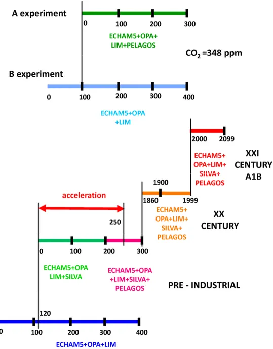
The coupled model described in Section 2.1 is used to produce a number of simulations which are shown schematically in Fig. 2-1. A coupled simulation containing the physical components only of the coupled model, i.e. atmosphere (ECHAM5), ocean (OPA 8.2) and sea ice (LIM), is named A for “abiotic”. Experiment A is initialized with climatological temperature and salinity data from the World Ocean Atlas 1998 (Antonov et al., 1998; Boyer et al., 1998) and is integrated for 400 years. Another coupled simulation is performed with the same physical core as experiment A with the addition of the marine biogeochemistry model PELAGOS and is named B for “biotic”. The B experiment is initialized with the physics of the year 100 of the A experiment and integrated further for 300 years. Both experiments A and B are conducted under constant greenhouse gas atmospheric concentrations, i.e. CO2, CH4, N20, and CFC; in

particular, CO2 concentrations are equal to 348 ppm, a value typical of the 1980s (Fig.

2-2). Marine biogeochemistry in experiment B is initialized as follows: macronutrients, dissolved inorganic carbon and alkalinity are prescribed from World Ocean Atlas 2001 climatologies (Conkright et al., 2002), dissolved iron concentration is initialized as homogeneous zonal bands based on sparse data collected by Gregg et al. (2003) and the remaining variables are set to uniform concentrations, with chlorophyll concentrations computed as a constant ratio of phytoplankton carbon. During the model integration, atmospheric iron deposition is taken into account by applying climatological model data from Tegen and Fung (1994) and assuming a dissolution fraction of 1%.

Figure 2-1: Experiments analyzed in this study: in experiments A and B atmospheric CO2

levels are set to 348 ppm; in the pre-industrial experiments greenhouse gases are set to the climatological value for the year 1860; in the “XX century” experiment greenhouse gases are those observed for the period 1860-1999; in the “XXI century” experiment greenhouse gases are prescribed according to the A1B scenario. Model components, used in different combinations among the simulations, are ECHAM5 (atmosphere), OPA 8.2 (ocean), LIM (sea ice), PELAGOS (marine biogeochemistry), SILVA (land and vegetation).

A set of centennial simulations have been performed within the framework of the EU Project ENSEMBLES (http://ensembles-eu.metoffice.com/). In particular, ENSEMBLES designed a carbon cycle concerted experiment, in which atmospheric greenhouse gases (hereafter GHG) concentrations are used to drive the carbon cycle model instead of GHG emissions, following the simulation strategy proposed by

Hibbard et al. (2007). A number of pre-industrial simulations were performed under climatological GHGs (CO2, CH4, N2O, and CFC), ozone, sulfate, and aerosol

concentrations relative to the year 1860, which for atmospheric CO2 is equal to 286

ppm. A pre-industrial simulation performed with the physical core of the coupled model was initialized following the method by Stouffer et al. (2004) from historical oceanic observations representative of current temperature and salinity distributions (Levitus et al., 1998). Another pre-industrial simulation containing the interactive terrestrial vegetation model SILVA was initialized from the year 120 of the physics-only pre-industrial experiment and integrated for 200 years. This simulation was used to initialize the physics and terrestrial vegetation of another pre-industrial experiment containing the interactive marine biogeochemistry model PELAGOS, where marine biogeochemistry was initialized identically as in the B experiment described above.

In order for the ocean and terrestrial biosphere carbon pools to equilibrate with preindustrial atmospheric CO2 concentrations, an artificial acceleration method was

performed, similarly to Alessandri (2006); specifically for the ocean, the global ocean-atmosphere CO2 fluxes drive an artificially enhanced ocean outgassing where the excess

carbon is removed homogeneously from the oceanic inorganic carbon pool. After the oceanic carbon pools have reached equilibrium with atmospheric GHGs, the simulation is continued for another 50 years and used to initialize a historical 1860-1999 century simulation containing all model components, and forced with observed atmospheric concentrations of atmospheric GHGs, sulphates, ozone, and aerosols (made available within the ENSEMBLES multi-model experiment). The year 1999 of the XX century is used to initialize a XXI century projected climate simulation performed with all components of the coupled model. Time-varying GHGs, sulphate, ozone, and aerosol concentrations are prescribed employing the Intergovernmental Panel on Climate Change (IPCC) Special Report on Emissions Scenarios (SRES) “business-as-usual” A1B scenario (Nakicenovic and Swart, 2000). The time evolution of atmospheric CO2

Fig. 2-2: Time evolution of prescribed atmospheric CO2 concentrations in the A and B

simulations, i.e. 348 ppm(black), for the 20th century simulation, i.e. those observed during the years 1860-1999 (blue), and for 21st century simulation according to the A1B scenario (red).

2.3 Model climatology and biases

Model climatologies are analyzed over the last 150 years of the B experiment and over the last 30 years of the XX century simulation, and compared with observational data sets. Fig. 2-3 shows in colors the annual SST bias with respect to 1950-2002 Hadley SST (Rayner et al., 2003) and the climatology of each experiment in contours. In the B experiment SST exhibits negative biases in the central equatorial Pacific (~2°C), in the northwestern North Atlantic (~6°C), in the northern Pacific subtropical gyre (~2°C) and in the Southern Ocean between 30°-60°S (2-3°C), and positive biases in the eastern tropical basins (~4°C) and in the North Pacific at around 45°N (~5°C). The last 30 years of the XX century exhibit similar spatial patterns even though the ocean surface is significantly colder. This counterintuitive result is due to the fact that sulfate aerosol concentration, exerting a negative feedback on surface temperatures, is higher in the last 30 years of the XX century than in the B experiment.

Fig. 2-3: Colors: Annual SST model bias (°C) with respect to Hadley SST, contours: model climatology; (a) B experiment, (b) last 30 years of the XX century.

Annual precipitation simulated in the B and XX century experiments is compared with Climate Prediction Center Merged Analysis of Precipitation (CMAP) estimates for 1979-2002 (Xie and Arkin, 1996) in Fig. 2-4. The model is capable of capturing the main features of the precipitation field even though precipitation in the Tropics is slightly overestimated and affected by the presence of a double Intertropical Convergence Zone (hereafter ITCZ), and over the North Atlantic and North Pacific storm tracks tend to be shifted more poleward than observed.

Similarly to other coarse resolution coupled simulations (Meehl et al., 2007), the SST and precipitation biases shown in Figs. 2-3 and 2-4 originate from issues regarding model physics, air-sea coupling and grid resolution. In particular, in the eastern tropical Pacific and Atlantic basins the misrepresentation of low stratus clouds and of deep convection processes could account for some of the SST and precipitation biases (Lin, 2007), whereas overly strong easterlies, simplified formulations of air-sea momentum fluxes (Jungclaus et al., 2006; Guilyardi et al., 2009) and reduced tropical instability wave activity are the likely cause for cold bias in the central equatorial Pacific. The North Atlantic negative SST bias is mostly related to the displaced pathways (Fig. 2-5) of the Gulf Stream and the North Atlantic Current (Reverdin et al., 2003) which reduce heat transport into the subpolar gyre.

Fig. 2-4: Simulated annual precipitation (mm day-1) in (a) B experiment, (b) last 30 years of the XX century (c) CMAP estimates.

Fig. 2-5: B experiment annual surface currents (m sec-2). Currents having a magnitude exceeding 0.65 m sec-1 are scaled of a factor 2 for better visualization (red arrows).

Annual wind stress biases with respect to ERA-40 reanalysis (Uppala et al., 2005) are shown in Fig. 2-6 for B and XX century experiments. In both the experiments, easterly trade winds in the northern subtropical Pacific are overestimated (up to 0.1 N m-2), and mid-latitude westerlies are poleward-shifted in the Northern Pacific and equatorward-shifted in the Southern Ocean. Wind biases are possibly originating from inaccurate meridional SST gradients which affect vertical shears of zonal winds through the thermal wind relation (Holton, 1992). Annual latent heat fluxes are compared with NCEP reanalysis (Kalnay et al., 1996), and their biases shown in Fig. 2-7 for B and XX century experiments together with their climatological values, where positive values indicate ocean heat gains. Latent heat losses tend to be overestimated where SST values are overestimated (e.g. subtropical gyres, Kuroshio extension region in the western North Pacific), whereas they tend to be underestimated where SST values are lower than observed (e.g. subpolar North Atlantic, equatorial Pacific).

Fig. 2-6: Simulated annual wind stress bias (N m-2) with respect to ERA-40 reanalysis (colors indicate magnitude) and model climatology (contours); (top) B experiment, (bottom) last 30 years of the XX century.

Fig. 2-7: Simulated annual latent heat flux bias (W m-2) with respect to NCEP reanalysis (colors) and model climatology (contours); (a) B experiment, (b) last 30 years of the XX century.

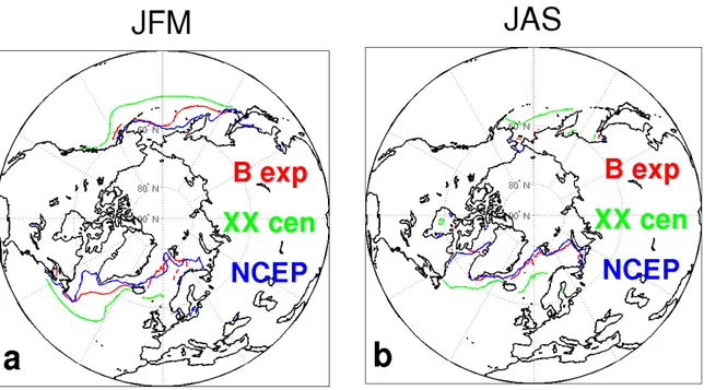
Fig. 2-8: sea ice edge, diagnosed as 1% sea ice cover for B experiment (red), last 30 years of the XX century experiment (green), NCEP reanalysis (blue) in January-March (JFM, left) and July-September (JAS, right).

The northern hemisphere sea ice edge, diagnosed as 1% sea ice cover, in B and XX century simulations is shown in Fig. 2-8 together with the NCEP reanalysis data (Kalnay et al., 1996) for winter (JFM) and summer (JAS) months. In the B experiment winter sea ice is generally overestimated in the Labrador Sea and in the western North Pacific whereas it is rather well simulated in summer. In the XX century sea ice is

highly overestimated in both the North Atlantic and North Pacific basins in relation to negative SST biases in the northern hemisphere (Fig. 2-3b).

Fig. 2-9: Mixed layer depth (m) plotted in logarithmic scale in January-March (JFM, left) and July-September (JAS, right) for (a,b) B experiment, (c,d) XX century experiment, and (e,f) de Boyer-Montégut et al. (2004) observational estimates.

Mixed layer depth (MLD) in B and XX century experiments is shown in logarithmic scale in Fig. 2-9 for January-March (JFM) and July-September (JAS) and compared with de Boyer-Montégut et al. (2004) estimates. It is to be remarked that MLD in the model is computed diagnostically as the depth at which ocean density is 0.1 kg m-3 higher than the surface, whereas in de Boyer Montégut et al. (2004) it is diagnosed as the depth at which temperature is 0.2 °C lower than the surface. As discussed by de Boyer Montégut et al. (2004), the temperature criterium is more suitable because of

higher spatial coverage of observational data and because it detects boundaries between density-compensated water masses.However MLD values calculated with two different methods (de Boyer Montégut et al., 2004) yield sufficiently similar results for the purpose of the present comparison. When compared with observational estimates, both the B and the XX century simulations show overestimation of JFM MLD in the Atlantic Nordic Seas and in the subpolar North Pacific, and underestimation in the Labrador Sea, the latter caused by overestimated sea ice (Fig. 2-8). In the Southern Ocean MLD is generally underestimated south of 60°S in both JFM (austral summer) and JAS (austral winter), and overestimated equatorward of 60°S in JAS (austral winter). The equatorward shift of MLD maximum in the Southern Ocean is possibly related to the incorrect equatorward displacement of westerly winds (Fig. 2-6).

Annual chlorophyll concentrations averaged over the euphotic layer depth in B and XX century experiments are shown in logarithmic scale in Fig. 2-10 and compared with SeaWiFS satellite estimates (McClain, 2009) and with World Ocean Atlas (Conkright et al., 2002) data averaged over the first 100 m depth. The main features of the chlorophyll field are correctly represented by the model simulation, in terms both of magnitude and of spatial structure, i.e. chlorophyll values are higher in subpolar regions (up to 0.5 mg m-3 in the North Pacific and Southern Ocean, up to 0.2 mg m-3 in the North Atlantic) and in the Tropics (up to 0.3 mg m-3 in the equatorial Pacific), and are lower at subtropical latitudes. However it may also be seen that chlorophyll values are underestimated at subtropical latitudes in both hemispheres, whereas they are overestimated south of 40°S in the Southern Ocean. In the North Atlantic Ocean chlorophyll values tend to be underestimated, even though the seasonal maximum is correctly captured in terms of both timing and amplitude (Fig. 2-11).

Fig. 2-10: Annual chlorophyll concentration in the euphotic layer (mg m-3) plotted in logarithmic for the (a) B experiment, (b) last 30 years of the XX century experiment, (c) SeaWiFS satellite estimates and (d) World Ocean Atlas observational data.

The reasons for the biases in the chlorophyll mean state arise from inaccuracies in both physical and biogeochemical models. For instance, the positive bias in the Southern Ocean is related to an inadequate representation of the mixed layer seasonal cycle, which is too deep in the winter months and too shallow in the subsequent summer months (Fig. 2-9). Moreover the equatorward displacement of the MLD maximum impacts the spatial distribution of the chlorophyll maximum as well. The chlorophyll underestimation in the subpolar North Atlantic Ocean is probably related to a number of reasons: (1) winter chlorophyll values are lower-than-observed because of the overestimated depth of the winter mixed layer (Fig. 2-11) which exerts a light limitation on phytoplankton growth; (2) the lower-than-observed summer values are related to underestimated nutrient concentrations (not shown) which are largely consumed and exported from the euphotic layer depth during the spring months; (3) in the course of the whole 300-year model integration, surface nutrient and chlorophyll values exhibit a systematic decrease, possibly caused by an overly strong export of nutrients from the surface layers into deeper ocean layers, where they are likely conveyed by the meridional overturning circulation towards south. This behavior may be seen in Fig.

2-12a showing a time series of B experiment chlorophyll concentration integrated in the euphotic layer and spatially averaged north of 35°N, where it may be seen that chlorophyll values tend to stabilize in the last 100 years of the simulation.

Fig. 2-11 Observed (blue, dashed line) and simulated (red, full line) climatological seasonal cycles, computed over the subpolar North Atlantic. Left: mixed layer depth (MLD) in m, where the observed values are from de Boyer Montégut et al. (2004). Right: chlorophyll concentration (Ch-SAT) in mg m-3, where observed values are SeaWiFS satellite estimates (McClain, 2009), and simulated values are vertically averaged until the 3rd optical depth.

It needs to be stressed that the goodness of a biogeochemical model lies in its capability of correctly simulating not only mean bulk biogeochemical properties but also the rates at which organic matter is processed within the food web, which influence upper ocean carbon transformation processes and ultimately carbon sequestration in deeper ocean layers. As shown by Vichi and Masina (2009), the PELAGOS model used in this study has skill at simulating net primary production over the global ocean, when compared with satellite-derived estimates and an independent data set of in situ observations in the equatorial Pacific.

For the analysis of chlorophyll interannual and decadal variability in the B experiment, characterized by constant atmospheric CO2 concentrations, it is convenient to have

chlorophyll anomaly time series detrended from systematic tendencies unrelated to climate variability. A second order polynomial fit of the last 200 years of the chlorophyll time series is therefore computed at each grid point and its spatial average north of 35°N shown Fig. 2-12a (red line). A fit with an exponential function was also

attempted but it did not give satisfactory results in all parts of the basin. Evidently, various time scales are involved in the adjustment process to initial conditions and thus one cannot assume a simple exponential model of chlorophyll temporal evolution in all grid points. The obtained polynomial coefficients are used to detrend the time series of B experiment chlorophyll concentration at each grid point. From Fig. 2-12b it may be seen that after the detrending operation over the last 200 years of the time series the chlorophyll anomalies oscillate around zero with fluctuations which are then related to climatic variability.

Fig. 2-12: Time series of annual chlorophyll (CHL) concentration integrated in the euphotic layer (mg m-2) and averaged north of 35°N. (a) B experiment CHL time series (black) and second order polynomial fit (red) over the last 200 years of simulation, (b) last 200 years of the B experiment CHL anomalies after detrending.

For the analysis of the marine biogeochemical response to increased CO2 concentrations

in the XXI century simulations, a polynomial fit of the time series cannot be performed as for experiment B. In fact the changes in surface chlorophyll are likely to be mostly forced by external climate trends. In Fig. 2-13 globally averaged time series of annual chlorophyll concentration values are shown for the pre-industrial simulation (where atmospheric gases and aerosols are climatologically set to the year 1860 values), for the historical simulation (where atmospheric gases and aerosols are those measured during the 1860-1999 period), and for the XXI century projection (where atmospheric gases and aerosols are those estimated by the A1B scenario). It has to be remembered that

marine biogeochemistry was initialized (identically as for the B experiment) at the beginning of the pre-industrial simulation. It may be seen that chlorophyll exhibits a large decrease during the first 100 years simulation, as similarly seen and discussed for the B experiment in the northern hemisphere (Fig. 2-12). Afterwards chlorophyll exhibits a tendency towards stabilization (as in the B experiment) before showing another large drop in the XXI century projection. It is very likely that the first chlorophyll drop in the pre-industrial era, i.e. performed under constant CO2

concentrations, is due to dynamics internal to the coupled model, whereas the second drop in the XXI century, i.e. after chlorophyll has roughly stabilized, is due to external climate forcing.

Fig. 2-13 Time series of annual chlorophyll concentration integrated over the euphotic layer depth and averaged over the global ocean (mg m-2) for the pre-industrial simulation (blue), historical simulation from 1860 to 1999 (green), and A1B scenario for the XXI century (red). Finally, a comparison between the simulated surface CO2 partial pressure (hereafter

pCO2) in the last 30 years of the XX century and observed pCO2 data obtained from the

Lamont Doherty Earth Observatory (LDEO) dataset (Takahashi et al., 2009a) covering the period 1970-2005 is shown in Fig. 2-14. Observed and simulated data are binned

onto a regular 2x2 degrees grid and annually averaged. The model reproduces the pattern of high pCO2 in the large scale upwelling of the Pacific Ocean, related to

entrainment to the surface of carbon-rich subsurface waters. It does not have skill however to reproduce the regions of high pCO2 in the Indian Ocean because of weaker

and shallower than observed upwelling, indicating that this area acts as sinks and not as source in the XX century simulation.

2-14 Maps of 2x2 degrees binned data of surface pCO2 (µatm) from (a) LDEO dataset

(Takahashi et al., 2009), (b) annual climatology of the last 30 years of the XX century simulation. From Vichi et al., 2010 (in preparation).

Chapter 3

Feedbacks of biological radiative heating in a

coupled climate model

Summary

This study addresses the mechanisms by which upper ocean phytoplankton may generate feedbacks on the global climate by means of solar radiation absorption during photosynthetic reactions. Phytoplankton radiation absorption gives rise to a local radiative heating pattern capable of propagating into the coupled and dynamical climate system and of generating feedbacks onto oceanic and atmospheric properties. Here a coupled model containing interactive marine biogeochemistry is used to perform a 300-year simulation which is compared with a physics-only simulation, thus enabling the analysis of the effects of the addition of biological radiative heating on the physical climate. It is found that in the dynamically coupled climate system the heating perturbation induced by biology propagates within the climate system and generates feedbacks on virtually all its components. A general increase of sea surface temperatures around 0.5°-1°C is accompanied by an enhancement of latent heat losses to the atmosphere which determine increases in atmospheric temperatures and water vapor content up to 6%. The equatorial maximum in biological heating causes an intensification of the Hadley circulation which acts as a teleconnection mechanism affecting cloudiness and solar radiation patterns from tropical to subtropical latitudes. Changes in temperature meridional gradients at extratropical latitudes modify the vertical shear of zonal winds and give rise to anticyclonic anomalies in the mid-latitude atmospheric circulation. Modified atmospheric circulation drives 5-10% modifications in the upper ocean circulation and related heat transports. In response to changes in incoming solar radiation and in ocean circulation, upper-ocean heat content decreases at tropical latitudes and increases at middle latitudes. The biologically-induced modifications in the physical climate might interact with the other sources of internal and external climate variability and might need to be kept into consideration in climate impact studies.

3.1 Introduction

The upper ocean contains a variety of living and dead particles which absorb, scatter and reflect incoming solar radiation (Morel and Antoine, 1994). Among these are chlorophyll pigments which are internal constituents of phytoplanktonic organisms used to absorb visible radiation for photosynthetic reactions. This process interacts with the vertical distribution of shortwave radiation through the water column and thus with the upper ocean heat budget. Bio-optical feedbacks are relevant in the context of climate research as they are virtually ubiquitous and intimately intertwined with time- and space-varying physical forcing factors.

Most climate models use a constant attenuation scale for visible radiation of ~20 m depth which comes from observational estimates of open ocean water clarity (Jerlov, 1968; Paulson and Simpson, 1977). This assumption however does not consider the large variations of bio-optical properties that can be found throughout the ocean on various temporal and spatial scales. For instance, local variations in temperature linked to biological radiative heating in the tropical Pacific were observed to strongly respond to ocean variability associated with El Niño Southern Oscillation (Strutton and Chavez, 2004); using remotely sensed data for the Arabian Sea, Sathyendranath et al. (1991) find that the distribution of phytoplankton, which is mainly governed by upwelling seasonality, exerts a controlling influence on the seasonal evolution of sea surface temperature.

Whereas the local effect of chlorophyll radiation absorption may be measured instrumentally, its full-scale effects on the climate system may only be addressed in modeling studies. A key region is the tropical Pacific, characterized by high chlorophyll concentrations and by pronounced ocean-atmosphere coupling. In forced ocean configurations biological heating was found to affect equatorial sea surface temperatures (Nakamoto et al., 2001; Loeptien et al., 2009) and it was suggested that this might improve some of the systematic errors found in coupled models (Murtugudde et al., 2002). The sea surface temperature (SST) response to biology is strongly dependent on dynamical feedbacks involving changes in mixed layer depth (hereafter MLD) and currents. It is found that changes in equatorial and off-equatorial MLD are connected to modifications of meridional ocean transports (Sweeney et al., 2005; Manizza et al., 2008; Loeptien et al., 2009) and zonal current velocities through geostrophic adjustment (Nakamoto et al., 2001; Lengaigne et al., 2007). In addition to

the local effect induced by biology on the Equator, non-local processes may also be important in affecting equatorial SSTs. For instance, the meridional advection of off-equatorial heat anomalies induced by biology is found to be relevant in affecting equatorial temperatures and their seasonal cycle (Sweeney et al., 2005; Lengaigne et al., 2007; Gnanadesikan and Anderson, 2009).

In the dynamically coupled ocean-atmosphere system, we also expect local biological heating anomalies to propagate into the climate system and generate feedbacks onto its components which are not easily predictable from the initial perturbation alone. In an atmospheric model forced by biologically-perturbed sea surface temperatures (Shell et al., 2003) and in coupled model experiments (Wetzel et al., 2006; Lengaigne et al., 2007; Gnanadesikan and Anderson, 2009) ocean biota generates changes in surface winds, in the Walker circulation, and in tropical precipitation patterns. The role of coupled ocean-atmosphere processes is however still not clear. On one hand the atmospheric response to biological heating is found to enhance temperature anomalies through wind stress feedbacks (Anderson et al., 2007; Lengaigne et al., 2007), on the other hand atmospheric feedbacks are found to weaken the biological perturbation through turbulent heat fluxes (Oschlies, 2004; Park et al., 2005). Finally, changes in the tropical ocean-atmosphere mean state may modify El Niño Southern Oscillation variability: hybrid and coupled models have been used to assess the role of ocean biota on tropical variability in response to changes in mean seasonal cycles (Marzeion et al., 2005; Lengaigne et al., 2007), air-sea coupling (Timmermann and Jin, 2002; Anderson et al., 2009), and thermocline depths (Wetzel et al. 2006).

A number of studies have focused on how biology interacts with the temperate and high latitude climate. Forced and coupled models containing interactive marine biogeochemistry were used to analyze biologically induced changes in ocean temperature, stratification, sea ice and ocean circulation (Oschlies, 2004; Wetzel et al., 2006; Manizza et al., 2008; Lengaigne et al., 2009). They find that the seasonal cycle of the MLD is amplified because of increased turbulent heat fluxes and changes in the ocean temperature vertical structure produced by biology. Spring biological heating is found to enhance sea ice melting and to produce freshwater anomalies which slightly impact the large-scale meridional overturning circulation (Lengaigne et al., 2009). Teleconnection processes with tropical latitudes arise in relation to Hadley circulation changes (Shell et al., 2003) which modify cloudiness and solar heat flux patterns at

surface temperatures anomalies induced by biology feed back on the wind stress curl field and thus play an indirect effect on ocean meridional overturning and water mass formation (Gnanadesikan and Anderson, 2009).

The understanding of how the global climate system as a whole responds to the bio-optical perturbation still remains a challenge. Even though the local effect of biological radiative heating has been observationally estimated by means of combined satellite and ocean measurements (e.g. Sathyendranath et al., 1991; Strutton and Chavez, 2004), the estimation of how this local effect may affect global climate is not possible in an observational framework as a “control” condition where biology is absent is not available. Yet the study of bio-optical feedbacks on the global climate is relevant in climate research as they may interact with the response of the Earth System to anthropogenic climate change.

The strategy in this study is thus to use a coupled ocean-atmosphere model containing interactive marine biogeochemistry which is capable of simulating the major interactions and feedbacks among different climate components on a global scale. The use of imposed chlorophyll structures would not be suitable for this study as it would not allow for internally consistent bio-physical feedbacks. A 300-year simulation containing full coupling with biology is compared with a physics-only control experiment with the purpose of analyzing bio-feedbacks on the adjusted state of a coupled climate system.

Scientific questions:

• Which regional responses arise in response to biological radiative heating? • Which are the oceanic and atmospheric mechanisms driving these responses? • Do these mechanisms act as positive or negative feedbacks on global temperatures?

This chapter is organized as follows: section 3.2 shows the biologically-induced changes in the ocean-atmosphere mean state. The discussion of dynamical mechanisms giving rise to these changes in the Tropics and Extratropics is deferred to Section 3.3. Section 3.4 briefly describes the impact of biological radiative heating on Tropical and Extratropical interannual variability. Concluding remarks are given in Section 3.5.

3.2 Changes in the ocean and atmosphere mean state

To assess the influence of interactive marine biogeochemistry on global climate, two 300-year simulations performed under constant CO2 atmospheric levels (described in

Section 2.3) are compared. The first is a physics-only control simulation and is named A for “Abiotic”; the second contains full interaction with marine biogeochemistry and is named B for “Biotic”. The last 150 years of each simulation are used for the analysis of all variables except heat trend terms which are available only for 100 years of simulation.

In experiment A ocean attenuation depth for visible radiation is held constant to 23 m, whereas in experiment B it varies spatially and temporally as a function of chlorophyll and detrital matter concentrations. In Fig. 3-1a we show B minus A attenuation depths calculated following equations 2-2 and 2-3 over the euphotic depth. A decrease in attenuation depths of 3 to 6 m occurs in correspondence of high chlorophyll structures, indicating an enhanced upper ocean heat trapping. Biological radiative heating the B experiment is computed the difference between total and “pure” seawater radiative heating. Areas of enhanced local biological radiative heating (Fig. 3-1b) occur in boreal and austral subpolar latitudes and in the equatorial Pacific, with annual mean values of 0.4-0.6 °C month-1 at the surface. We remark that radiative heating is only one of the components of the upper ocean heat budget alongside advective, diffusive and ocean-atmosphere heat fluxes: these other terms compensate for excess radiative heating in order to maintain the climate system in dynamical equilibrium. Biological radiative heating is the only difference between the two experiments and its effect on oceanic and atmospheric properties will now be described. The discussion of local and remote mechanisms leading to these changes will be deferred to Section 3.3.

The addition of biology to the coupled model overall warms the ocean surface (Fig. 3-2a). In the eastern tropical Pacific and at middle and subpolar latitudes SST in experiment B is ~0.4°C higher than in A, with peaks of more than 1°C in some localized regions of the North Pacific and North Atlantic Oceans. SST differences are instead close to zero or negative in some limited areas at high latitudes and in the tropical Pacific Ocean. Following SST changes, the ocean is in general more stratified in experiment B with respect to A (Fig. 3-2b), especially at middle and subpolar latitudes and in the central equatorial Pacific, where percentual changes in mixed layer depth (hereafter MLD) may reach 20%. Heat content integrated between the surface and

300 m depth (Fig. 3-2c) is higher by ~5×108J m-2 at subtropical and middle latitudes, whereas it tends to be lower (~3×108 J m-2) at tropical latitudes (20°S-20°N) and poleward of 50°S and 50°N. Heat content changes arise from the complex interplay of oceanic and atmospheric mechanisms, as discussed in the next section. B minus A differences in SST, heat content and MLD are statistically significant at 99% on large portions of the global ocean (Fig. 3-3), where statistical significance is determined by means of a Student’s t-test.

Fig. 3-1: (top) B minus A annual mean differences of attenuation depth (m); (bottom) B experiment biological heating at the surface (°C month-1).

Fig. 3-2: B minus A annual mean differences of (a) sea surface temperature (SST) in °C, (b) mixed layer depth (MLD), indicated as the percentual change with respect to the A experiment, (c) 0-300 m integrated heat content (HC) in J m-2, (d) precipitation (PREC), in mm day-1, (e) solar radiation at the ocean surface (W m-2) and (f) ocean-atmosphere latent heat fluxes (W m-2), where positive heat fluxes indicate an ocean heat gain.

Feedbacks on atmospheric variables and on air-sea heat fluxes are also detected. Precipitation (Fig. 3-2d) increases by more than 0.3 mm day-1 between 10°S-10°N in the Pacific, whereas it generally decreases between 15°-30° in both hemispheres. Changes

appear in general to respond to local SST changes and the Intertropical Convergence Zone (ITCZ) is not significantly displaced. Incoming solar radiation at the ocean surface (Fig. 3-2e) is overall lower at tropical latitudes (except on the equatorial Pacific) whereas it is higher at subtropical and middle latitudes. Changes in incoming shortwave radiation in experiment B are connected to the vertical integral of cloud cover (not shown), which is up to 2% higher in the tropical belt (except on the equatorial Pacific) and down to 2% lower at subtropical and middle latitudes. Changes in cloudiness are related to atmospheric circulation changes, as it will be discussed in the next section. Ocean-atmosphere latent heat fluxes (Fig. 3-2f) - defined positive downwards – in general decrease in B, indicating that an ocean with biology looses more heat to the atmosphere through evaporative fluxes. Some limited areas of positive B minus A latent fluxes occur however in the tropical Pacific, in northwestern Atlantic Ocean and in the Southern Ocean. In most areas, solar and non-solar heat flux changes range between ±5 W m-2.

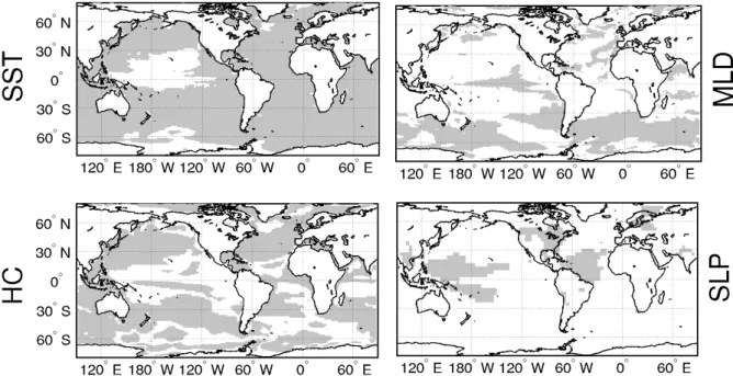
Fig. 3-3 Statistical significance at a 99% confidence interval of B minus A annual mean differences of (a) sea surface temperature (SST), (b) mixed layer depth (MLD), (c) 0-300 m integrated heat content (HC), (d) sea level pressure (SLP).

The presence of biology induces anomalies in surface atmospheric circulation through changes in wind velocities (Fig. 3-4, arrows). Wind patterns appear to respond to sea level pressure changes (Fig. 3-5), whose relation with biological heating will be discussed in Section 3.3. Sea level pressure changes are in general statistically not

significant at extratropical latitudes and in the eastern parts of the tropical basins (Fig. 3-3d), where interannual fluctuations exceed changes due to biology. At extratropical latitudes, increased sea level pressure is associated with negative wind stress curl anomalies (Fig. 3-4, colors) in the northern hemisphere (positive in the southern hemisphere), indicating increased anticyclonic vorticity of surface winds. Wind speed changes are around 0.5 m sec-1, i.e. 5-10% with respect to the A experiment. At tropical latitudes wind changes in B with respect to A are especially high in the Pacific Ocean (differences up to 1 m sec-1). Sea level pressure decreases in the eastern Pacific and increases in the central part of the basin, causing westerly wind anomalies to arise east of 130°W. In the central-western Pacific sea level pressure in B is relatively lower on the equator with respect to subtropical latitudes, causing increased wind convergence on the Equator. Easterlies are then weakened in the eastern part of the basin, whereas in the central-western part of the basin they increase their magnitude and their convergence on the Equator.

Fig. 3-4: B minus A annual differences of wind velocities in m sec-1 at 1000 mbar (arrows) and associated wind stress curl in 1×10-8 N m-3 (colors).

Changes in wind patterns may in turn affect ocean circulation through changes in wind stress curl (Fig. 3-4, colors). At middle latitudes (between 40°-60°), negative wind stress curl changes of 1-2×10-8 N m-3 in the northern hemisphere (positive in the