RR Lyrae stars in M31 field and globular clusters: How did Andromeda form?

(1)

UNIVERSIT `

A DI BOLOGNA

Facolt`

a di Scienze Matematiche Fisiche e Naturali

Dipartimento di Astronomia

Dottorato di Ricerca in Astronomia Ciclo XXII (2007-2009)

RR LYRAE STARS IN M31 FIELD

AND GLOBULAR CLUSTERS:

HOW DID ANDROMEDA FORM?

Tesi di Dottorato di

Rodrigo Contreras Ramos

Coordinatore: Chiar.mo Prof. Lauro Moscardini

Relatore: Chiar.mo Prof. Bruno Marano

Co-Relatori: Dott.ssa Gisella Clementini

Dott.ssa Luciana Federici

Esame Finale Anno 2010

SCUOLA DI DOTTORATO IN SCIENZE MATEMATICHE, FISICHE E ASTRONOMICHE SETTORE SCIENTIFICO DISCIPLINARE: AREA 02 - SCIENZE FISICHE

(2)

(3)

(4)

Introduction

As the nearest giant spiral galaxy, Andromeda (M31) provides a unique opportunity to study the structure and evolution of a massive galaxy and, by comparison with the Milky Way (MW), to address the question of variety in the evolutionary histories of massive spirals. Our external view of this system offers a significant advantage, since it reduces complications due to projec-tion and/or line-of-sight effects, that plague the MW studies and, as a result, the structures observed in M31 are easier to study, thus making Andromeda the best current laboratory for investigating faint stellar structures around galaxies.

At a distance of about 800 kpc, M31 is close enough that individual stars in the galaxy field can be resolved and measured with 8m-class telescopes like the Large Binocular Telescope (LBT), reaching the horizontal branch (HB) of the old stellar populations with less than half an hour exposures. Resolving individual stars in the M31 globular clusters (GCs) or in crowded fields requires instead the Hubble Space Telescope (HST).

van den Bergh (2000, 2006) suggested that Andromeda originated as an early merger of two or more relatively massive metal-rich progenitors. This would account for the wide range in metallicity (Durrell, Harris, & Pritchet 2001) and age (Brown et al. 2003) observed in the M31 halo, compared to the MW. M31 hosts spectacular signatures of present and past merging events like the giant tidal stream (Ibata et al. 2001) extending several degrees from the center of the galaxy (McConnachie et al. 2003), and the arc-like overdensity connecting the galaxy to its dwarf elliptical companion NGC205 (McConnachie et al. 2004).

(8)

Ferguson et al. (2002) and Ibata et al. (2007) presented the first panoramic views of the Andromeda galaxy, based on deep Isaac Newton Telescope (INT) and Canada-France-Hawaii Telescope (CFHT) photometric observations that cover respectively the galaxy inner 55 kpc, and the southern quadrant out to about 150 kpc, with an extension that reaches M33 at a distance of about 200 kpc. Their data show the giant stream in all its extension and reveal also a multitude of streams, arcs and many other large-scale structures of low surface brightness, as well as two new M31 dwarf companions (And XV and And XVI).

The primary tool to understand the formation history of a galaxy is the analysis of color mag-nitude diagrams (CMDs) deep to the main-sequence turn-off (TO) of the oldest populations. However, the TO of the oldest stars in M31 (V ∼ 28.5 mag) is still unreachable by the largest ground-based telescopes, and required hundred orbits of HST/ACS time entirely devoted to “tiny” (3′_{.5 × 3}′_{.7) portions of the galaxy (Brown et al. 2003, 2006, 2008).}

The pulsating variable stars may offer a powerful alternative tool to trace stars of different age in a galaxy since variables of different types arise from parent populations of different age (old: RR Lyrae stars and Population II Cepheids; intermediate age: Anomalous Cepheids – ACs –; young: Classical Cepheids). The RR Lyrae stars, in particular, belonging to the oldest stellar population (t > 10 Gyr), have eyewitnessed the formation of their host galaxies, and thus can allow to reconstruct the star formation history (SFH) back to the first epochs of galaxy forma-tion. These variables are also about 3 magnitude brighter, hence much more easy to observe, than coeval TO stars, and the typical form of their light variation makes them much more easy to recognize than old non-variable stars, in crowded fields dominated by younger stars.

My PhD thesis is part of a large project aimed at studing the variable star population in prop-erly selected fields and globular clusters of the Andromeda galaxy. The Wide Field Planetary Camera 2 (WFPC2) on board the HST has been used to resolve and study variable stars in six M31 globular clusters (GCs), and the wide field capabilities of the LBT were used to study the field star population in selected areas of the M31 halo and giant stream. The study of the M31 variable stars, and in particular the study of the pulsation properties of the RR Lyrae stars

(9)

holds a crucial role for identifying the “building blocks” of galactic halos and for understanding which galaxy formation scenario (merger/accretion or cloud collapse) is dominant. In the MW almost all GCs which contain significant numbers of RR Lyrae stars sharply divide into two very distinct classes, the Oosterhoff types (Oosterhoff 1939), according to the mean pulsation periods of their RR Lyrae stars, and it is likely that this dichotomy reflects conditions within the MW halo at the time of GC formation.

In M31 the situation is completely unknown. We do not really know whether the M31 GCs show the Oosterhoff dichotomy, or whether indeed they can be placed into Oosterhoff groups at all, since no studies have been yet made that define the properties of RR Lyrae stars in the GCs of M31, and the RR Lyrae that have been identified so far in M31 both from ground-based and HST studies (Pritchet & van den Bergh 1987, Dolphin et al. 2004, Brown et al. 2004, Vilardell et al. 2007, Joshi et al. 2009, Sarajedini et al. 2009) all belong to the field population. Based on our HST and LBT data, this thesis work will try to answer the following questions: i) Is the Oosterhoff dichotomy a general characteristic of old cluster populations in spiral galaxies similar to our own, or it is a peculiar phenomenon due to the particular evolutionary history of the MW? ii) Do the pulsation properties of the RR Lyrae stars in the M31 GCs correlate with metallicity as in the Galactic GCs? iii) Can we demostrate that the RR Lyrae stars in the MW and M31 field and GCs share the same properties, and assume this properties as universal in the definition and calibration of the Population II distance scale?

The thesis is organized in 6 chapters and 9 Appendices. The first 3 chapters describe the thesis scientific background. In particular, in Chapter 1, we present a general overview of the 2 main galaxy formation scenarios for the case of the Milky Way. Then, in Chapter 2 we describe the main properties of different types of intrinsic variable stars, and discuss how they can be used in the context of the present thesis. Finally, in Chapter 3 we give a general picture of Andromeda (M31), the galaxy that hosts the targets selected of our study. We also include a brief summary of the works found in literature concerning the study of the RR Lyrae stars in

(10)

Andromeda, and conclude the chapter giving the scientific motivations of this thesis work. The second block of 3 chapters forms the heart of the thesis. These chapters describe all the work done and the results obtained in the thesis. Specifically, Chapter 4 describes the study of the variable stars, in particular of RR Lyrae type, in 6 properly selected globular clusters in M31, for which time-series photometry was obtained with the Hubble Space Telescope. In Chapter 5, we focus on the variability study of 2 selected M31 fields, sampling respectively a region close to the giant stream, and the galaxy halo, for which time-series data were obtained with the Large Binocular Telescope. Finally, Chapter 6 gathers the main conclusions of this study, and the related future work. At the end of the thesis, 9 Appendices present the atlas of light curves for each of our selected targets.

(11)

How do galaxies form? The case of

the Milky Way

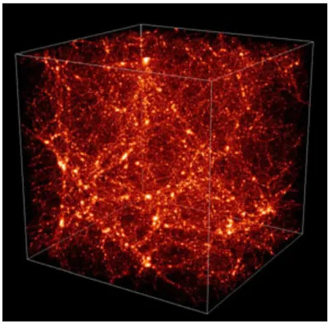
One of the greatest unanswered questions in astrophysics concerns the formation and evolution of galaxies in the Universe. Today it is believed that galaxies, as well as other structures in the Universe, have been formed out of primordial density fluctuations that have grown under the influence of gravity. As the Universe expanded the average density of the cosmic gas would have declined, however, some density enhancements of sufficient size, became more pronounced, thanks to their own gravitational attraction. This attracted matter from surrounding regions, increased still further the lumpiness of the Universe. This process, known as gravitational instability, was therefore responsible for the production of localized regions in which clouds of cosmic gas collapsed despite the general background of expansion (see Fig. 1.1). These collapsing clouds are the supposed seeds of the galaxies and clusters of galaxies.

So, how did these collapsing clouds give rise to the galaxies that we see today? The simplest scenario for galaxy formation is that the collapse of a single over-dense region gives rise to a single galaxy. The mass contained in such a region would therefore correspond to the mass of the resulting galaxy. This type of formation process is often referred to as monolithic collapse

(12)

Figure 1.1: The effect of gravitational instabilities in a region of the expanding Universe dominated by dark matter. Regions of enhanced density tend to grow along with the general cosmic expansion, but if sufficiently dense they may eventually defy the expansion and collapse.

scenario. However, the way in which gravitational collapse proceeds depends on the distribution of mass, therefore the most dominant form of matter in the Universe, the dark matter, should play the key role in this process. From the theoretical point of view, two different dynamical behaviors of the dark matter may affect the growth of gravitational instabilities. In one, dark matter consists of slow moving, massive particles. This kind of dark matter is referred as cold dark matter (CMD). The term cold refers to the fact that the hypothetical dark matter particles have random speeds that are small compared with the speed of light. Simulations of

(13)

gravitational collapse, in a Universe dominated by CDM, reveal that the first structures to form have masses of the order of 106M⊙, which is 5 orders of magnitude lower than those typically

found for galaxies in the present-day Universe. As time progresses, large scale features develop by further collapse and by merger of the lower mass structures that were form previously. The overall picture is one in which proto-galactic fragments form early in the history of the Universe and many of the galaxies we see today are the results of merging events. This type of process is termed hierarchical scenario or bottom-up scenario, since galaxies are generally formed by amalgamation of smaller entities. The other extreme behavior is one in which the dark matter particles are rapidly moving, and goes under the name of hot dark matter (HDM). The term hot refers to the fact that dark matter particles have speeds that are comparable to the speed of light. One effect of these high speeds is to remove small scale density fluctuations. In this case, the model prediction is that the first entities to form in the Universe would have much larger masses than individual galaxies. Structures with masses similar to the present-day galaxies would form by the fragmentation of these large entities. This type of process is called top-down scenario.

The currently favored theory is that structures in the Universe formed in a bottom-up scenario under the influence of CDM. In such a scenario the first objects formed might be very high mass stars, followed by structures on the scale of GCs and small systems like the dwarf spheroidal galaxies (dSphs). Large galaxies would then form by merging of these smaller components.

1.1 Cloud Collapse Model for the Milky Way

The general notion that the MW reached its present form after a gravity collapse from a more dispersed state dates back at least to Kant (1755). This classical view of the formation of the Galaxy has been given a modern interpretation and quantification by Eggen, Lynden-Bell and Sandage (ELS), after having studied the motion of a sample of high velocity stars in the MW halo (Eggen et al. 1962). They found a correlation between ultraviolet excess and eccentricities

(14)

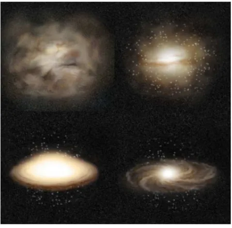
Figure 1.2: Schematic figure showing the Cloud Collapse scenario in four stages, from upper left to lower right (taken from Krauss & Chaboyer 2003).

in the sense that stars with the largest UV excess (i.e., lowest metal abundance) are moving in highly elliptical orbits, whereas stars with little or no UV excess move in nearly circular orbits. A correlation between UV excess and angular momentum was also found: stars with large UV excesses have small angular momentum.

Based on these correlations they proposed that the original proto-Galaxy consisted of a single large spinning, metal poor gas cloud with a radius (in present day coordinates) of about 100 kpc. This cloud, unable to support itself by gas pressure, once its mass had stopped the local Hubble expansion, immediately underwent a free-fall collapse (see Fig. 1.2). Stars that formed

(15)

in the early stages of the collapse of the protogalactic gas cloud inherit the low metallicity and predominantly radial motion of the inward falling gas, and are seen today as randomly oriented, elliptical orbiting, small angular momentum metal-poor halo stars. The GC and field halo stars are supposed to have formed in condensations embedded within the intra-Galactic medium dur-ing this free-fall phase. As the cloud collapsed, its rate of spin increased to conserve its angular momentum, and at the same time, supernova explosions increased slowly the content of metals in the cloud. As a consequence, successive generations of stars formed by this enriched gas, are both closer to the center of the galaxy and increasingly metal rich (radial metallicity gradient). Finally, when the gas achieved a density which allowed pressure support, and dissipation there-fore began to become important, it was able to radiate away its kinetic energy; residual angular momentum then forced it to settle into a rotating disk, where all subsequent star and cluster formation has taken place. Metal-rich stars would form in this disk as the interstellar medium is enriched with the products of nucleosynthesis during stellar evolution. In contrast to the gas, the disipationless halo field stars and GCs have retained the kinetic energies, angular momenta, and general spatial distribution that they possessed at the instant the gaseous collapse ceased. According to this scenario, the collapse was very quick, with a duration that could have not exceeded a few times 108 years, which translates in a very small spread in age among halo stars and GCs.

1.2 Hierarchical Model for the Milky Way

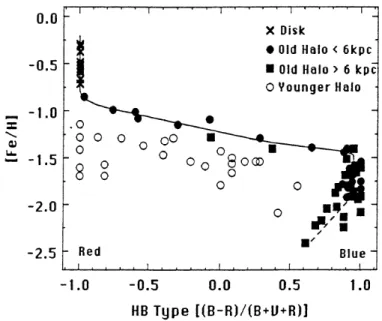
An alternative scenario for the formation of the MW was proposed by Searle & Zinn (SZ) in 1978. They measured and compiled the most up-to-date and reliable metal abundances and horizontal branch (HB) morphologies1 available at the time for about 50 Galactic GCs, and

1

The HB morphology is characterized by HB-type defined as: HB-type=(B − R)/(B + V + R), where V is the number of RR Lyrae stars, and B and R are the numbers of HB stars respectively bluer and redder than the RR Lyrae instability strip.

(16)

Figure 1.3: Subdivision in the HB morphology versus metal abundance plane of the MW halo GCs ([Fe/H< −0.8) (taken from Zinn 1993).

investigated these properties as a function of galactocentric distance, RGC. Surprisingly, they

found no radial abundance gradient in the cluster system in the outer halo (RGC &8 kpc), as

would be expected for the cloud collapse model. They also found significant differences in HB morphology between inner and outer halo GCs. This effect is shown in Fig. 1.3, where it is clearly visible that GCs in the inner regions of the Galaxy follow a tight relationship between HB morphology and metallicity, whereas clusters at larger galactocentric radii have in the mean, more red HB types at a given metallicity (the so called “second parameter problem”) and exhibit a considerable scatter between these 2 quantities2. This body of evidence points towards the possibility of two populations of halo GCs. Note that the inner/outer halo dichotomy appears

2

From this plot arose one of the most successful classification scheme for the Galactic GCs: those systems that follow the fiducial line which traces the relationship between HB-type and [Fe/H] for the inner halo clusters are called “old” GCs, while those that clearly deviate form the “young” halo components.

(17)

to be well-supported by field stars as well (Carollo et al. 2007). According to early HB models, the observed range in HB morphological types would require that the epoch of GC formation has lasted much more than 1 Gyr, and therefore the formation of the Galactic halo could not have been as rapid as a free-fall collapse. Thus, as suggested by SZ, the large spread in HB-type is best understood as a difference in age, with the red HB outer halo GCs several Gyrs younger than the blue HB counterpart at large radii, as well as the inner halo clusters. In order to explain the required prolonging of cluster formation time, SZ adopted a model assuming that the outer halo formed over a longer period of time via the capture of external systems or “protogalactic fragments”, and that the red HB outer halo clusters originated in satellite systems that were subsequently accreted by the MW. This model is known today as the hierarchical picture, since big galaxies form by merging and accretion of small entities or “building blocks” (see Fig. 1.4). The spread in HB morphology of GCs can be explained by different star formation histories in the accreted systems. It is also theorized that a significant fraction of halo field stars were once members of a GC. We now know that GCs do indeed disrupt, the most clear example being that of Pal 5 (Odenkirchen et al. 2003). As noted by Zinn (1980), obvious candidates for these “building blocks” are the present-day dwarf spheroidal (dSph) and dwarf irregular (dIrr) galaxies. Such galaxies are the most numerous in the Universe and the dSphs in particular are found to surround both the MW and M31 in large numbers (although their numbers fail by an order of magnitude or more to match those predicted by ΛCDM theories (Klypin et al. 1999). There are undoubtedly other faint dwarfs still to be found, and the Sloan Digital Sky Survey has recently allowed to discover several of them around the MW (see e.g., Willman et al. 2005; Kleyna et al. 2005; Belokurov 2006, Belokurov et al. 2007). However, it is unlikely that the numbers required by the ΛCDM theories really exist, although the most recent estimate (Simon & Geha 2007) suggests that there is only a factor of 4 too few dwarf galaxies currently known. Many of the newly discovered MW dSph satellites are known to contain a sizeable fraction of stars that are similar to those in the MW halo, namely old and metal-poor.

(18)

Figure 1.4: A giant elliptical galaxy in the cluster Abell 3287 in the process of hierarchical growing. The partially digested remnants of several cannibalized galaxies are visible in the central region (taken from West et al. 2004).

which is currently being accreted by the MW (Ibata et al. 1995). This dwarf galaxy is not only contributing to the Galaxy with field stars, but also with a handful of GCs; some of which showing a quite young age. This example of recent “cannibalism” suggests that the Galaxy is still in the process of formation an that young GCs in the outer halo can also be accounted for if the SZ model is invoked. Less evident but equally suggestive is the case of ω Centauri, both the brightest and the largest GC associated with our Galaxy, known so far. It has been speculated that this peculiar cluster may be the core of a dwarf galaxy which was disrupted and absorbed

(19)

by the MW (see, e.g. Villanova et al. 2007). Also interesting is the case of Terzan 5. Very recently Ferraro et el. (2010) have claimed that this GC could be the surviving remnant of one of the primordial “building blocks” that are thought to have merged to form the Galactic bulge. This case is particularly interesting since it suggests that the subsystems hypothesized by SZ may actually have been the “building blocks” not just of the Galactic halo, but of the entire Galaxy.

1.3 “Building Blocks” of The Milky Way

In order to probe the predictions of the SZ theory for the Galaxy formation, an obvious test is to compare the main properties of the present-day dSph or dIrr systems surrounding the MW with those of the MW halo stars. If the MW halo was indeed made up in large part by dissolved systems initially resembling the dSphs or dIrrs we see today, one would expect to find many similarities in their stellar populations.

One approach is the direct comparison of the detailed chemical composition of stars from the two environments, based on spectroscopy. If the halo formed from dSphs or dIrrs or objects like them, their chemical makeups should be similar. Such a study has been dubbed “chemical tagging” by Freeman & Bland-Hawthorn (2002). The catchphrase “near-field cosmology” also applies, as we are probing cosmological galaxy formation theories using the nearest galaxies as our testbeds. The alpha-elements (e.g., O, Mg, Si, Ca, and Ti) are specially useful for this pur-pose because their abundance is an indicator of the star’s enrichment history. The production of these elements is dominated by Type II supernovae, while iron has important contributions by both Type II and Type Ia supernovae. Thus, the ratio of alpha-elements to iron, [α/Fe], is commonly used to trace the star-formation timescale in a system, because it is sensitive to the ratio of SNe II (massive stars) to SNe Ia (intermediate-mass binary systems with mass transfer) that have occurred in the past. The salient feature of these comparisons is that the halo abun-dances are essentially unique. The general α vs. [Fe/H] pattern of most of the dwarf galaxies

(20)

Figure 1.5: [Mg/H] and [Ca/H] vs. [Fe/H] for samples of stars in four different dwarf galaxies. α-elements in extragalactic samples are generally depleted with respect to their Galactic counterparts (taken from Tolstoy et al. 2009).

studied are very different from that of the MW halo stars. More specifically, the [α/Fe] ratios of stars in dSph galaxies are generally lower than those of similar metallicity Galactic stars (see Fig.1.5). In the same vein, the Galactic halo contains a significant fraction of stars more metal-poor than [Fe/H] ∼ −2.5 (see, e.g., Christlieb et al. 2004; Beers et al. 2005), including a not negligible tail of stars with metal abundances even lower than −3.0 (see Helmi et at. 2006 and references therein), while the dSphs, on the other hand, contain very few metal-poor stars (see, e.g., Tolstoy et al. 2004; Koch & Grebel 2006), with a significant lack of stars with metallicities below [Fe/H] ∼ −3.0 (Helmi et al. 2006; Aoki et al. 2009).

Another approach is the comparison of the stellar populations. In trying to relate the young, metal-rich populations observed in the halo with the stellar population of the present-day dSphs, Unavane et al. (1996) recognized that the Galactic halo contains a negligible amount of young stars in comparison with the vast majority of old components, unlike most of the MW’s satellite dSph galaxies which often do contain sizeable numbers of young stars. Thus, they estimate that, at the most, only 6 Fornax-type progenitors or 60 Carina’s could have been accreted by

(21)

the Galaxy. This is in contradiction to the predictions of the hierarchical model, in terms of both the number and the mass spectrum of the contributors needed to produce a MW-type halo (Unavane et al. 1996; Gilmore & Wyse 1998). Similar discrepancies between stellar pop-ulations in the dSphs satellites and the MW halo are found when comparing the numbers of intermediate-age giant carbon stars, since the Galatic halo is apparently less abundant in these stars than the present-day dwarf satellites (van den Bergh 1994).

All the arguments mentioned above cast some doubts on the possibility that the dwarf galaxies we see today in the surrounding of the MW and M31 could be the hierarchical protogalactic fragment candidates. However, these arguments hide some obvious limitations; the younger and intermediate-age stars we see today were not present when the bulk of the halo formed. In fact, the halo progenitors or Galactic “building blocks” may not be replicas of present-day satellite galaxies. As pointed out by Mateo (1996), the present-day dSphs are survivors, and therefore special conditions must have precluded them from disruption (late accretion and/or less-radial orbital characteristics). These conditions could have allowed the present-day dSphs to follow a different evolutionary path than the original “building blocks”. A difference in time of formation alone, for example, could explain the lack of intermediate and young populations in the halo relative to the present-day satellites (van den Bergh 1994; Majewski et al. 2002). In the same vein, the satellites that have survived may have undergone additional chemical enrichment over a prolonged time span. Running the clock back to the time when the MW halo was forming, a Sculptor-type galaxy would have looked very different. Accordingly, these arguments concerning the role of dwarf galaxies in the assembling of the Galaxy only provides us with information about a “relatively recent” part of the overall history.

Thus, in order to place meaningful constraints on the way our undoubtedly old Galactic halo formed, one should really compare those stars which saw what really happened at the beginning, and survived to this day to tell us the whole truth about the matter. In other words, we should compare the very oldest stars in both the present-day halo and the MW dwarf companions. Un-mistakable old, with ages comparable to the age of the Universe, the RR Lyrae stars are ideal

(22)

candidates to this purpose. If the Galaxy formed by the accretion of protogalactic fragments that resembled the MW dwarf satellites as they were ∼ 10 Gyr ago, then the pulsation prop-erties of the RR Lyrae stars in the Galactic halo and in the dwarf galaxies should be basically indistinguishable.

1.3.1 RR Lyrae Stars: Real Eyewitnesses of galaxy formation

In the present section we compare the properties of the RR Lyrae stars in the Galactic GCs with the properties of the RR Lyrae stars belonging to GCs and general field of the MW dwarf satellites. The left panel of Figure 1.6 presents the distribution of the mean periods of the ab-type RR Lyrae (RRab) stars for Galactic GCs containing at least 5 RR Lyrae as a function of the cluster’s metallicities. Except for the peculiar positions of the clusters NGC 6441 and NGC 6388, labeled as OoIII in the figure, it is clear from this plot that the MW globulars present the so called Oosterhoff dichotomy (Oosterhoff 1939), i.e. the lack of systems with average period of the RRab stars in the range from 0.58 days to 0.62 days. Only four GCs out of 41, or less than 10%, are found inside the “Oosterhoff gap”, two of which are quite peculiar: M75 has a trimodal horizontal branch (Corwin et al. 2003), whereas the metal poor cluster Rup106 appears younger than other typical metal-poor Galactic globulars by about 4-5 Gyr (Buonanno et al. 1990) and is suggested to be connect with the stream of the Sagittarius dSph (Bellazzini et al. 2003). The right panel of Fig. 1.6, on the other hand, shows those nearby extragalactic system possessing their own GC systems, namely, the Large and Small Magellanic Cloud (LMC and SMC, respectively) dIrr’s, the Fornax and Sagittarius dSphs, and the recently discover Canis Major overdensity and its suggested GC system3 _{(Martin et al. 2004). From the plot, it becomes}

clear that these massive dwarf galaxies in the immediate vicinity of the MW show a very different picture. For instance, the LMC GCs show a continuous trend in RR Lyrae properties rather than an Oosterhoff dichotomy. In the case of Fornax (see e.g., Greco 2007), the GCs preferentially

3_{The true nature of the Canis Major overdensity, whether an actual dwarf galaxy or the MW warp, is still}

(23)

Figure 1.6: Left panel: Oosterhoff type I, II and III Galactic GCs in the hP abi versus [Fe/H] diagram. Clusters containing relatively small numbers of RR Lyrae are plotted using smaller dots. Right panel: same as in the previous plot, but now including dwarf satellites of the MW and their GCs. These extragalactic objects preferentially occupy the Oosterhoff gap region, in stark contrast with the Galactic GCs (taken from Catelan 2009).

occupy the Oosterhoff intermediate region which is almost avoided by the Galactic GCs. This immediately rules out the possibility that any building blocks of the MW may have resembled the LMC or Fornax some 13 Gyr ago, otherwise the Oosterhoff dichotomy would not exist. In fact, in the case of external systems, almost 50% of them are found inside the “Oosterhoff gap”. Similar conclusions may be reached when considering the stellar fields of the remaining 7 less massive dwarf MW companions: Ursa Minor, Draco, Carina, Leo II, Sculptor, Leo I and Sextans. All of them, but Ursa Minor, have been classified as Oosterhoff intermediate objects (see eg., Catelan 2009 and references therein). In summary, the distribution of mean periods of the RRab stars for the Galactic and nearby extragalactic systems is undoubtedly different. The Oosterhoff dichotomy is not present among the satellite companions of the MW. Thus, these results seems to definitely ruled out the present-day dSph galaxies as the possible protogalactic

(24)

fragments invoked by SZ. While we do see evidence of ongoing mergers between some dSphs (e.g., Sagittarius, Ibata et al. 1995) and the Galaxy, the Oosterhoff argument suggests that these must not have provided a major contribution to the stellar content of the MW halo.

1.3.2 New Pieces of the Puzzle, New Clues

Prior to the Sloan Digital Sky Survey (SDSS; York et al. 2000), the number of known MW dSph satellites had been increasing at a rate of one or two per decade, reaching the total number of only ten widely accepted MW dSph satellites. The small number of known companions surrounding the Galaxy is one of the biggest problems of the ΛCMD model, often referred as the “missing satellite problem” (Klypin et al. 1999, Moore et al. 1999). Indeed, in the current ΛCMD paradigm of structure formation, dark matter halos of the mass of the MW dSph galaxies outnumber the known dSphs by a factor of 10-100 (Penarrubia, Navarro, & McConnachie 2000, and references therein). Since 2005, 17 new dSph satellites of the MW have been discovered, primarily from the analysis of images obtained by the SDSS: Willman I, Ursa Major I (UMa I), Ursa Major II (UMa II), Bootes I, Coma Berenices (Coma), Segue I, Canes Venatici I (CVn I), Canes Venatici II (CVn II), Leo IV, Hercules, Leo T, Bootes II, Leo V, Bootes III, Segue II, Pisces I, and Pisces II (Willman et al. 2005a, 2005b; Zucker et al. 2006a, 2006b; Grillmair 2006, 2009; Belokurov et al. 2006, 2007, 2008, 2009; Irwin et al. 2007; Walsh et al. 2007; Watkins et al. 2009; Belokurov et al. 2010). They have eluded previous discovery because they all have very low surface brightness (µv &28 mag arcsec−2). Being so faint they have been

named “ultra-faint” dSphs (UFDs). The new galaxies are mainly concentrated around the North Galactic pole, as this is the region observed by the SDSS. After the discovery of the new systems, the dSph galaxies surrounding the MW have been divided into two main groups: “bright” or “classical” dSphs, already known before 2005, and “ultra-faint” dSphs, discovered in the last three-four years. Classical and ultra-faint dSphs lie in two separate regions in the absolute magnitude versus half-light radius plane (see Figure 1.7). UFDs have small velocity dispersions,

(25)

Figure 1.7: Location of different classes of objects in the plane of absolute magnitude vs half-light radius. Lines of constant surface brightness are marked. Open circles and open squares are the bright dSphs surrounding the MW and M31, respectively. Filled circles are the “ultra-faint” Milky Way (MW) dSphs satellites, and two extremely low luminosity globular clusters, discovered after 2005, mainly from the analysis of SDSS data (see text). Bold open squares are new M31 dSph satellites discovered after 2004 (see Chapter 3). Open triangles are Galactic globular clusters (GCs) from Harris (1996), and Mackey & van den Bergh (2005). Filled stars are GCs of the Andromeda galaxy, from Federici et al. (2007). Open stars are GCs in the outer halo of M31, from Mackey et al. (2007) and Martin et al. (2006). Asteriscs are extended M31 GCs, from Huxor et al. (2005) with parameters measured by Mackey et al. (2006). Cyan filled circles are GCs of NGC5128, from McLaughlin et al. (2008). Magenta filled inverted triangles are nuclei of dwarf elliptical galaxies in the Virgo cluster, from Cote et al. (2006). Diamonds are ultra-compact dwarfs in the Fornax cluster, from De Propris et al. (2005). (taken from Clementini 2010).

(26)

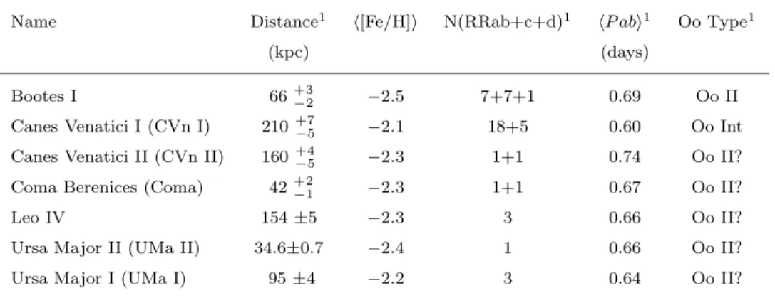
Table 1.1: Oosterhoff properties of RR Lyrae stars in the “ultra-faint” MW dSphs

Name Distance1 _h[Fe/H]i _N(RRab+c+d)1 _{hP abi}1 _{Oo Type}1

(kpc) (days)

Bootes I 66+3

−2 −2.5 7+7+1 0.69 Oo II

Canes Venatici I (CVn I) 210+7

−5 −2.1 18+5 0.60 Oo Int

Canes Venatici II (CVn II) 160+4−5 −2.3 1+1 0.74 Oo II?

Coma Berenices (Coma) 42+2−1 −2.3 1+1 0.67 Oo II?

Leo IV 154 ±5 −2.3 3 0.66 Oo II?

Ursa Major II (UMa II) 34.6±0.7 −2.4 1 0.66 Oo II? Ursa Major I (UMa I) 95 ±4 −2.2 3 0.64 Oo II?

1_{Distances and properties of the RR Lyrae stars are from Dall’Ora et al. (2006) for Bootes I; from Kuehn et al. (2008) for}

CVn I; from Greco et al. (2008) for CVn II; from Musella et al. (2009) for Coma, from Moretti et al. (2009) for Leo IV; from Dall’Ora et al. (2009) for UMa II; and from Garofalo (2009) for UMa I. Question marks indicate the difficulty of classifying these galaxies due the small number of variables they contain (taken from Clementini 2010).

3-4 km/s, showing dark matter dominance, and have distorted morphologies, probably due to the tidal interaction with the MW. They all host an ancient stellar population with chemical properties similar to that of external Galactic halo stars (Simon & Geha 2007; Kirby et al. 2008; Frebel et al. 2009). Several of the UFDs have mean metallicities as low or lower than the most metal-poor GCs and, generally, much lower than those of the classical dSphs. Furthermore, the α/Fe ratios of extremely metal-poor stars in the ultra-faint dwarf spheroidals are as high as those found in the bulk of Galactic halo stars (Frebel et al. 2009), while the abundance ratios between α-elements and iron in the most metal-poor stars found in the classical dSphs are lower than those found in Galactic halo stars (Aoki et al. 2009). Seven of the UFDs have been searched for variable stars so far (namely, Bootes I, Dall’Ora et al. 2006, Siegel 2006; CVn I, Kuehn et al. 2008; CVn II, Greco et al. 2008; Coma, Musella et al. 2009; Leo IV, Moretti et al. 2009; UMa I, Dall’Ora et al. 2009; and UMa II, Garofalo 2009) and only with the exception of CVn I, were all found to contain RR Lyrae stars with properties resembling those of the MW Oosterhoff II GCs, although one must be aware that this Oosterhoff classification is

(27)

more insecure than in the case of the classical dSphs, given the few RR Lyrae stars found in the UFDs. All of the above characteristics suggest that a much larger population of objects similar to the present-day UFDs, as they were at earlier times, may have been the “building blocks” of the halos of large galaxies such as the MW. The association is particularly clear with the outer halo of the MW, which Carollo et al. (2007) have demonstrated to exhibit a peak metallicity of [Fe/H]= −2.2, substantially lower than the inner halo, whose metal abundance peaks at [Fe/H]= −1.6, and which is the dominant population at Galactocentric distances beyond 15-20 kpc. Last but not least, the SDSS discoveries could have a bearing on the “missing satellite” problem. In fact, the SDSS present-day sky coverage is only about 1/4 of the celestial sphere, simple statistical arguments suggest that many more UFDs likely exist at latitudes not yet explored and could potentially fill the gap between theoretical expectations and observational evidence. In conclusion, it seems plausible that a population of ultra-faint, dark dwarf galaxies really does surround the MW. Only after a complete census of these objects has been obtained will we be able to assess whether their number and properties are consistent with the predictions of the simulations.

(28)

Variable Stars as Tools.

All stars display variations of brightness and color in the course of their evolution. Variable stars are traditionally devided into two main categories: intrinsic and extrinsic variables. The former vary due to causes internal to their structure and, among them, pulsating stars are characterized by periodic or cyclic variations. In particular, radially pulsating stars have pulsation periods typically ranging from hours to hundreds of days, and pulsation amplitudes of hundredths to ∼ 1 mag. They share a common locus that runs almost vertical in the HR diagram, named instability strip (IS), due to the fact that they also share the same pulsation mechanism, associated to opacity variations in the ionization regions of H, He and HeI.

Pulsating stars obey to a period- mean density relation that is at the basis of their use as stellar population tracers and distance indicators. In fact, assuming the Stephan Boltzman law combined with the period-mean density relation one obtains a relation between the period, the mass, the luminosity and the effective temperature. If the mass and the luminosity are related to each other, as in the case of Classical Cepheids, a period-luminosity-color relation is expected. Moreover neglecting the color dependence, or averaging over the color extension, one obtains a period-luminosity relation. This implies that the study of the pulsation properties of variable stars can help us to constrain the distance of the host systems, as well as the intrinsic

(29)

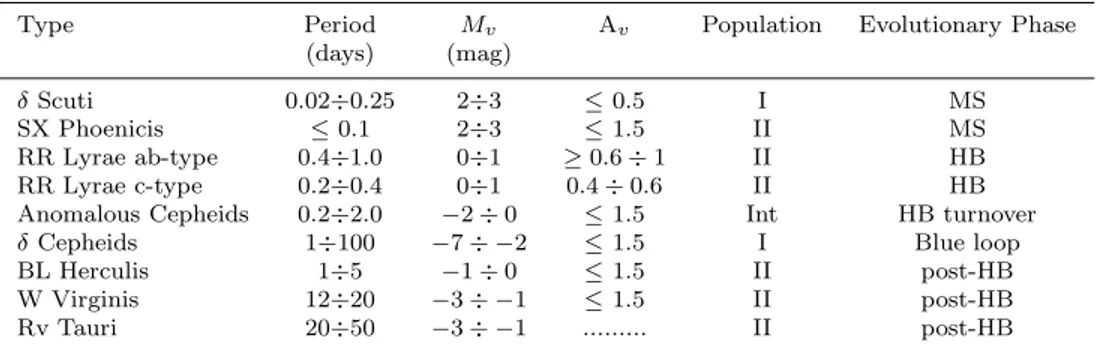
Table 2.1: Main characteristics of different types of pulsating variables found in the Classical Instability strip

Type Period Mv Av Population Evolutionary Phase

(days) (mag)

δ Scuti 0.02÷0.25 2÷3 ≤ 0.5 I MS

SX Phoenicis ≤ 0.1 2÷3 ≤ 1.5 II MS

RR Lyrae ab-type 0.4÷1.0 0÷1 ≥ 0.6 ÷ 1 II HB RR Lyrae c-type 0.2÷0.4 0÷1 0.4 ÷ 0.6 II HB Anomalous Cepheids 0.2÷2.0 −2 ÷ 0 ≤ 1.5 Int HB turnover

δ Cepheids 1÷100 −7 ÷ −2 ≤ 1.5 I Blue loop

BL Herculis 1÷5 −1 ÷ 0 ≤ 1.5 II post-HB

W Virginis 12÷20 −3 ÷ −1 ≤ 1.5 II post-HB

Rv Tauri 20÷50 −3 ÷ −1 ... II post-HB

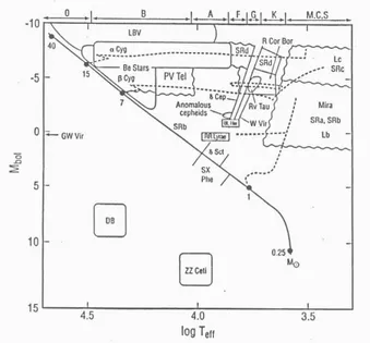
evolutionary properties of the investigated stars. The study of pulsating variables based on times series may allow to map the 3D structures and to characterize the spatial distribution of the different types of variables in a galaxy, providing information on the spatial distribution and time confinement of the burst of their parent populations. Furthermore, since different types of variables in the classical instability strip are in different evolutionary phases and belong to different stellar populations, they can be used as tracers of the different components in a stellar system: RR Lyrae stars and the Type II Cepheids tracing the oldest stars (t > 10 Gyr); the Anomalous Cepheids (ACs) tracing the intermediate-age component (∼ 1 − 5 Gyrs); and the Classical Cepheids representing the young stellar population (50-200 Myrs). The role of these variable stars can become crucial when the stellar population is not as simple as in a globular cluster (GC), and stars with different ages and metallicities share the same region of the CMD. The detection of different classes of pulsating variables may allow to identify different star formation episodes that have occurred in the host stellar system. Table 2.1 shows and owerview of the currently known major types of pulsating variables, along with their main characteristics and Fig. 2.1 illustrates the loci occupied by them in the HR diagram. In the following subsections, we present a briefly description of the variable stars that we have detected in this thesis.

(30)

Figure 2.1: Position of different types of pulsating stars in the HR diagram.

2.1 Classical Cepheids

Cepheids are high-luminosity, radially pulsating variable stars, with periods ranging between 1-100 days, and commonly associated with relatively young stellar populations like those found in open clusters, disk of spiral galaxies or in irregular galaxies. Their presence in star clusters allows their ages to be estimated as up to about 108 _{yr. From the stellar evolution point of}

view, these variables are intermediate-mass (3 − 12M⊙) stars that cross the instability strip

during the helium burning phase. In particular, after the quiescent ignition of He at the core by the 3α reaction, these stars may make an excursion toward higher effective temperature and, subsequently come back toward the asymptotic giant branch in the HR diagram. This “loop” may extend to sufficiently high temperature (or blue color) to intersect the instability strip in which case the stars become classical Cepheids. Their intrinsic brightnesses range from −2 > MV > −7, making them ideal distance indicators on Galactic and extragalactic scales. In

(31)

fact, they are observable up to distances of 20-30 Mpc (see e.g. Freedman et al. 2001). The close relationship between period and luminosity which was found by Henrietta S. Leavitt in 1912, has given the Classical Cepheids a unique role in establishing the distances to the nearer galaxies, and hence the distance scale of the Universe. On this basis they provide the absolute calibration of important secondary distance indicators, such as the maximum luminosity of supernovae Ia, the Tully-Fisher relation, surface brightness fluctuations, and the planetary nebulae luminosity function, that are the basis for measurement of the Hubble constant (Freedman et al. 2001; Saha et al. 2001). A very debated issue is the universality of the period-luminosity relation and in particular the effect of the metallicity on its coefficients, because any systematic effect affecting the Cepheid period-luminosity is expected to have relevant consequences on the extragalactic distance scale and the estimate of the Hubble constant. Cepheids are also good tracers of intermediate-mass stars in the Galactic disk (Kraft & Schmidt 1963), and star-forming regions in extragalactic systems (Elmegreen & Efremov 1996). The use of Cepheids as tracers of young stellar populations was soundly supplemented by the evidence that if these objects obey to a PL relation, and to a Mass-Luminosity relation, they also obey to a Period-Age relation. In particular, an increase in period implies an increase in luminosity, i.e., an increase in the stellar mass, and in turn a decrease in the Cepheid age.

2.2 Type II Cepheids

Type II Cepheids have periods between 1 and 26 d and are observed in GCs with few RR Lyrae stars. They are brighter than the RR Lyrae stars with similar metal content and are often divided into two classes: BL Her stars (P < 1) and W Vir (P > 1). As reviewed by Wallerstein (2002) they originate from hot, low mass stellar structures that started the main central He burning phase bluer than the RR Lyrae gap and now evolve toward the AGB crossing the pulsation region with luminosity and effective temperature that increase with decreasing the mass (see also Di Criscienzo, Marconi, Caputo, Cassisi 2007).

(32)

Type II Cepheids are widely believed to be the immediate progeny of low mass HB stars (M ∼ 0.53M⊙), but with mass still enough to reach the AGB stage, i.e., blue HB stars. This is

supported both by the observational record, which shows that type II Cepheids are present only when a sizeable blue HB component is also present (Wallerstein 1970; Smith & Wehlau 1985), seemingly irrespective of the metallicity (Pritzl et al. 2002; 2003); and by theoretical models (Schwarzschild & Harm 1970; Gingold 1976; 1985). Accordingly, detection of type II Cepheids should immediately imply the presence of a sizeable blue HB component.

These pulsating variable stars consist of three subclasses in different evolutionary stages, namely, BL Herculis (BL Her), W Virgins (W Vir) and RV Tauri (RV Tau) stars. Their evolutionary status can be summarized as follows: Stars on the horizontal branch, bluer than the RR Lyrae gap, evolve toward higher luminosity and larger radius (just like stars leaving the main sequence) as they deplete the helium in their cores. In doing so they cross the instability strip at a luminosity that corresponds to a period between roughly 1 and 5 days. This accounts for the short-period group, namely, BL Her of low metallicity. The origin of BL Her of near-solar metallicity remains uncertain, since they are likely to originate from the red horizontal branch. After reaching the AGB they advance to higher luminosity and begin to suffer helium shell flashes, which cause the star to make an excursion into the instability strip. The luminosity at which this occurs results in stars having periods between 12 and about 20 days. These are the so called W Vir variable stars. The paucity of Type II Cepheids with periods between 5 and 12 days, especially in the globular clusters, can be understood as the lack of shell flashes until the star’s luminosity reaches that which corresponds to a 12 day period. As the star becomes more luminous, mass loss reduces the remaining hydrogen shell to around 0.01M⊙ , whereupon the

star begins its travel across the top of the HR diagram around MV = −3.5 to -4.5, heading to the

white dwarf cooling sequence. While doing so it passes through the instability strip once again, now with a period of 20-50 days (which is often listed as twice that because of their behavior of alternating deep and shallow minima). These are the RV Tau stars, and are easily recognizable by their alternating deep and shallow minima of their light curves. (Wallerstein 2002; Soszynski

(33)

Figure 2.2: Period-Luminosity diagrams for Cepheids in the LMC. Green, blue, cyan and magenta symbols show type II Cepheids; red and orange symbols represent anomalous Cepheids; and grey points Classical Cepheids (taken from Soszynski et al. 2008)

(34)

et al. 2008). Since these variables obey a P-L relation, they can be used as standard candles to find distances (see Fig. 2.2). However, as illustrated in the plots, the P-L relation is not linear for the whole range of periods covered by type II Cepheids, and actually the P-L relations should be fitted separately for BL Her, W Vir and RV Tau stars. This is is especially valid for RV Tau stars which seem to be much brighter than would be expected from the extrapolated relation fitted to shorter-period type II Cepheids (e.g., Demers and Harris 1974, Alcock et al. 1998).

2.3 Anomalous Cepheids

Anomalous Cepheids (ACs) are radialy pulsating variable stars commonly observed in Local Group galaxies containing metal poor stellar populations. Their pulsation periods range from ∼ 0.2 to 2 days and they are typically 0.5-1.5 mag brighter than the RR Lyrae stars in a system. The origin of their anomaly lies in the evidence of being more luminous, for the same period, than Type II Cepheids tipically observed in old and metal poor stellar clusters, like GCs. The ACs follow their own P-L relation, both for fundamental mode pulsators and first overtone ones (Pritzl et a. 2002), which runs between the type I and type II Cepheid P-L relations (see Fig. 2.2).

A general consensus exists in the literature (see, e.g., Bono et al. 1997, Caputo 1998, and refer-ences therein) on the fact that AC variables, like RR Lyrae stars and Population II Cepheids, are metal-poor He-burning stars in the post Zero Age Horizontal Branch (ZAHB) evolution-ary phase. As reviewed by Caputo (1998), for low metal abundances (Z < 0.0004) and rel-atively young ages (< 4 Gyr) the effective temperature of ZAHB models reaches a minimum (log T e ∼ 3.764) for a mass of about 1.0-1.2 M⊙, while if the mass increases above this value,

both the luminosity and the effective temperature start increasing, forming the so called ZAHB turnover. For larger metallicities, the more massive ZAHB structures have brighter luminosities but effective temperatures rather close to the minimum effective temperature. Within such an

(35)

evolutionary scenario, the ACs appear to belong to the post-turnover portion of the ZAHB which crosses the instability strip at luminosity higher than the RR Lyrae pulsators. Their origin is still debated and the most widely accepted interpretations are: (1) they are young (∼5 Gyr) single stars due to recent star formation; (2) they formed from mass transfer in binary systems as old as the other stars in the same stellar system. Their pulsation properties allow us to use them as distance indicators and tracers of intermediate age stellar populations (see Marconi, Fiorentino, & Caputo 2001).

While ACs are almost nonexistent in GCs, they are common in dSph galaxies. Every dSph surveyed for variable stars has been shown to include at least one AC. As recently suggested by Dolphin et al. (2002) and theoretically confirmed by Caputo et al. (2004) ACs are indeed the extension to the lowest metallicities of the short period Classical Cepheids observed for example in the Magellanic Clouds.

2.4 RR Lyrae stars

RR Lyrae are low mass He burning stars on the HB evolutionary phase. They are important distance indicators and tracers of the properties of the old stellar populations. Their role as standard candles is twofold: i) their absolute visual magnitude is a relatively well known func-tion of the metal content; ii) they obey to a PL relafunc-tion in the near infrared bands. Their periods range between about 0.2 days and 1 day, and since Bailey (1902) they are divided in two main classes: RRab with relatively high amplitude (0.4 < Av < 1.5) decreasing with the

period, periods ranging from ∼ 0.4 to 1 day, and asymmetric light curve shapes; and RRc, with amplitudes ranging from 0.2 < Av < 0.6 mag, periods around 0.2-0.4 days, and sinusoidal light

curve shapes. The theory of pulsation has shown that RRab pulsate in the fundamental mode, while RRc pulsate in the first overtone. In addition there are also double-mode variables, pul-sating simultaneously in the fundamental and first overtone modes, and it has also been suggest that RR Lyrae stars may pulsate in the second overtone (e.g., Alcock et al. 1996,; Clement &

(36)

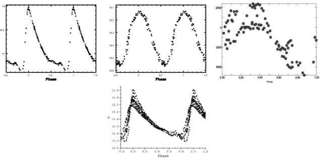
Rowe 2000). An intriguing and not well understood phenomenon is the so called Blazhko effect present in some RR Lyrae, and consisting in a periodic modulation, on a much longer timescale than the primary period, of the light curve shape. The Blazhko period falls in the range between ∼ 5 days and 530 days. Fig. 2.3 illustrated the different types of RR Lyrae stars. According to evolutionary models, these variables are the progeny of stars that begin their life in the main sequence with a mass near 0.8 M⊙. Like other low-mass stars, they spend most of their lifetime

in this sequence burning H into He in their cores and, after perhaps ∼ 10 Gyr, they climb the RGB where the core temperature becomes high enough to initiate helium fusion with a flash. Via the 3α reactions helium burning is ignited in a degenerate core and these reactions induces a violent re-adjustment in the giant structure, and the stars will contract toward their ZAHB location, where a new equilibrium is attained burning helium into carbon at the centre, and hy-drogen into helium in a shell surrounding the helium-rich core. According to this scenario, RR

-0.5 0 0.5 1 1.5 17 16.5 16 -0.5 0 0.5 1 1.5 16.6 16.5 16.4 16.3 16.2 16.1

Figure 2.3: Examples of RR Lyrae star light curves: RRab, upper left; RRc, upper center; RRd, upper right; and Blazhko RR Lyrae, lower center.

(37)

Lyrae variables are unanimously recognized as HB stars that cross the instability strip during their central He-burning evolutionary phase.

Being part of the oldest stars in the Universe, they have long been known to be present in large numbers in GCs, and to represent the ancient population in systems composed by stars of different ages and compositions. Accordingly, they can be used as ideal tracers of the old com-ponent (t > 10) in the MW and external galaxies. On the other hand, as stated above, they are important primary distance indicators due to their characteristic variability and to the fact that their mean brightness has been known to be nearly constant in any given GC since a century ago. Nowadays, it is widely accepted that the RR Lyrae visual magnitude has an approximately linear dependence on metallicity (see Caputo et al. 2000, for a non linear dependence) and that evolutionary effects must also be take into account. For our purposes, we assume that the Mv(RR)−[F e/H] is linear, with the slope value estimated by Clementini et al. (2003) and

Grat-ton et al. (2004), and the zero point value consistent with a distance modulus for the LMC of 18.52± 0.09 mag (Clementini et al. 2003), i.e. Mv(RR) = (0.214 ± 0.047)[F e/H] + (0.86 ± 0.12).

Fiinally, as already mentioned, RR Lyrae stars are characterized by a quite narrow PL relation in the near-infrared bands that has been found to be sensitive to metallicity (see e.g. Bono et al. 2003, Sollima et al. 2006.)

2.4.1 The Oosterhoff Dicothomy

Seventy years ago, P.Th.Oosterhoff discovered that the Galactic GCs could be divided into two groups according to the mean periods of their RR Lyrae stars. Studying a sample of only 5 GCs, he published a short paper giving just“some remarks on the variable stars in GCs” (Oosterhooff 1939), obviously unaware that his discovery could be hiding a recipe for understanding the formation of the MW. In this paper, he classified those clusters whose fundamental mode RR Lyrae stars showed mean periods, hPabi, close to 0.55 days (M3, M5) as Oosterhoff I (OoI), while

(38)

II (OoII). Differences in the mean periods of the RRc variables (hPci) in these clusters were also

present. Oo I clusters had RRc mean periods near 0.32 days, while those classified as OoII, showed mean periods close to 0.37 days. He also noted that the percentage of c-type variables differed between the two groups, in the sense that the RR Lyrae populations in OoI clusters were largely dominated by ab-type pulsators whereas OoII clusters generally contained a more balanced proportion between c and ab-type pulsators, although he was aware that incompleteness and selection effects may alter this property. Though the sample of clusters originally examined by Oosterhoff was small, subsequent works (Oosterhoff 1944, Sawer 1944) including new RR Lyrae-rich GCs soon confirmed the dichotomy. When in the 1950s metal abundances began to be determined for GCs, it became evident that these two classes were associated with differences in metallicity. OoI clusters were moderately poor, while OoII clusters were very metal-poor. A summary of the Oosterhoff properties of the MW GCs is provided in table 2.4.1. The most recent studies (see e.g., Cetalan 2009, for a review), involving larger samples of GCs, more accurate metallicities, precise periods for the RR Lyrae stars, and better completeness, have fully confirmed the Oosterhoff dichotomy not only for GCs, but also for the halo field stars in the MW. In Figure 2.4, hPabi is plotted against [Fe/H] for GCs containing a significant number (at

least 10) of RR Lyrae stars. The separation into two Oosterhoff groups is evident, as well as the so-called “Oosterhoff gap”, the region that covers the period range between 0.58 . hPabi . 0.62,

that is basically avoided by Galactic GCs. Note that the figure shows also a gap for metallicities between −1.6 . [Fe/H] . −1.9. The reason for this feature is that GCs with metal abundances in this range generally have horizontal branches which are extremely to the blue of the instability

Table 2.2: General properties of Oofterhoff I and II GCs Type hPabi hPci n(c)/n(ab + c) [Fe/H]

(days) (days)

OoI 0.55 0.32 0.17 &−1.6

(39)

Figure 2.4: Oosterhoff dicothomy in GCs (left) and in the field (right). Only GCs with at least 10 RRab are plotted, except for the OoIII globular cluster NGC 6388 with has only 9 RR Lyrae stars. In the plot with the field variables, period shifts were measured with respect to the M3 RR Lyrae stars (taken from Catelan 2004).

strip, and hence have very few RR L yrae stars. On the other hand, metal-rich glubular clusters such as 47 Tuc ([Fe/H]=-0.7) have most of the time stubby red horizontal branches that fall almost entirely to the red side of the instability strip, and thus have almost no RR Lyrae at all. Interesting however, are the cases of the GCs NGC6388 and NGC6441 which have [Fe/H] values of −0.6 and −0.5 dex, respectively. Despite their high metallicities, they have blue HB components in addition to the red horizontal branch usually seen in GCs of that metallicity. This blue extension crosses the instability strip, so that numerous RR Lyrae stars occur in both clusters, and unexpectedly, their values of hPabi are among the longest known for any cluster.

Because of their bizarre position in the [Fe/H]-hPabi diagram, they have defined a new class of

objects; the Oosterhoff type III GCs (Pritzl et al. 2000).

(40)

Lyrae variables, fc ≡ Nc/(Nc+ Nab). This plot suggests that, while there is a trend for OoI

clusters to have smaller values of fc than OoII clusters, practically any value of fc is allowed for

both OoI and OoII clusters, thus suggesting that, fc is not a good diagnostic of the Oosterhoff

status. Likewise, the left panel of Figure 2.5 shows the run of hPabi with the average c-type

period hPci. As can be clearly seen from this plot, hPci does not appear to be a good Oosterhoff

indicator either. Note that, since the pioneering work of Oosterhoff (1939, 1944), these two parameters have been considered important indicators of the Oosterhoff status. Finally, the right panel of Figure 2.5 shows the correlation between hPabi and the corresponding shortest

period of the ab-type stars Pab,min, that indicates the transition period between RRab and RRc

variables. As can clearly be seen, there is not only a strong global correlation between these two quantities, but also a strong correlation within each Oosterhoff group. Therefore, it seems that Pab,min along with hPabi are the most important quantities defining the Oosterhoff behavior.

Figure 2.5: The average period of ab-type RR Lyrae stars hPabi as a function of: (Left) average period of c-type

stars; (Center) fraction of c-type pulsators with respect to the total number of RR Lyrae stars; and (Right) as a funtion of the minimum period of the RRab stars, Pab,min. The only clear correlation exists for hPabi vs. Pab,min

(41)

2.4.2 Physical Origin of the Oosterhoff Dicothomy

Although much time has passed since the discovery of the dichotomy in Galactic GCs, its physical origin is still controversial. According to Sandage (1993) the dichotomy was due to a difference in period between individual ab pulsators at fixed effective temperature. Taking into account the van Albada & Backer equation (1971), this implied a difference in luminosity higher than what expected on the basis of the canonical evolutionary scenario, and with the unpleasant consequence that Y should be anti-correlated with Z (see Bono et al. 1995, for a discussion). The favored theoretical explanation for the Oosterhoff phenomenon is related to a sort of hysteresis mechanism (van Albada & Backer 1973). According to this explanation, the Oosterhoff dichotomy is due to a different distribution of ab and c pulsators in the OR region, that is the region of intersection between the fundamental and the first overtone in the instability strip, where in principle both pulsation modes are efficient. In particular in OoI GCs the OR region is expected to be mainly populated by RRab, whereas in OoII GCs it should be mainly populated by RRc. This different behavior should be caused by an hysteresis mechanism according to which in the OR region the pulsation mode is determined by the star’s previous evolutionary path (see left panel of Fig. 2.6). Thus, RRab stars entering the OR region from the red side continue to pulsate in the fundamental mode until they reach the blue edge of the fundamental mode, and then become RRc stars. On the other hand, RRc variables entering the OR region from the blue side, continue to pulsate in the first overtone mode until they reach the red edge of the first overtone mode, where they start to pulsate in the fundamental mode. This mechanism would naturally explain the Oosterhoff groups if RR Lyrae stars in OoII clusters are evolving redward from a position mainly on the blue side of the HB, whereas those RR Lyrae stars in OoI clusters contain a mix of unevolved and blueward evolving stars. The right panel of Fig. 2.6, shows schematically the situation for a single evolutionary track. As one can see, in cases a), b) and c) periods come from both low (unevolved) and high (evolved) luminosity pulsators, while in c) and d) an abrupt increase in mean periods of the fundamental pulsators is expected

(42)

Figure 2.6: Left panel: Schematic diagram illustrating the pulsation zones inside the instability strip under the hysteresis mechanism proposed by van Albada & Backer. Right panel: An example of how the instability region is populated by RRab (filled dots) and RRc (open dots) during the main phase of the HB evolution, under the hysteresis mechanism (taken from Caputo et al. 1978).

because the contribution of lower (unevolved) luminosity ab-type pulsators suddenly disappears. We note that the Hysteresis scenario is supported by the results of nonlinear convective pulsation models (see Bono et al. 1995, Bono et al. 1997).

2.4.3 What causes the Oosterhoff dichotomy in the MW?

Sandage et al. (1981) argued that RR Lyrae stars in OoII clusters had longer periods mainly because they were more luminosus than those in OoI clusters. The higher luminosity in OoII group should be caused by the low metallicity of these clusters, even if the amount of over-luminosity required to explain the Sandage period effect was to high to be explained by the canonical evolutionary scenario. This has been generalized to a relation between [Fe/H] and absolute V magnitude hMvi, for the RR Lyrae stars, with the more metal poor pulsators also

being intrinsically brighter. On the other side, Lee et al. (1990) concluded, from the study of horizontal branch models, that the Oosterhoff dichotomy is instead a morphological issue: RR Lyrae variables in OoII GCs, with their predominantly blue HB types, are evolved away from a position on the blue zero-age horizontal branch (ZAHB), and therefore, they cross the instability

(43)

strip at higher luminosities (and lower masses) and thus their periods are longer. Conversely, RR Lyrae stars in OoI clusters, with their uniformly populated or red HB morphologies, are mostly “unevolved” or ZAHB objects, which translates into lower luminosities and therefore lower periods. Thus the Oosterhoff type, is determined not by the metallicity of the cluster but rather by the HB type. Whether the metallicity or the HB morphology or a combination of both effects is controlling the Oosterhoff status of a GC is still unclear. While Lee & Carney (1999) showed that for the case of GCs with similar metallicities but very different horizontal branch morphologies, the Oosterhoff classification is determined by the latter, Contreras et al. (2005; 2010), on the other hand, concluded that metallicity, at a fixed HB type, is a key parameter determining the Oosterhoff status of a GC. Consequently, both [Fe/H] and HB type are respon-sible for the observed period dichotomy, as the evolutionary effects are crucial in determining the Oo type.

2.4.4 The Oosterhoff dichotomy: a formation dichotomy?

Further studies on the Oosterhoff dichotomy have revealed that the well defined Oosterhoff groups have also differences in age, spatial distributions, kinematics and even origin. Lee & Carney (1999) discussed the kinematic differences between Oosterhoff group I and II clusters (see left panel of Fig. 2.7). Their results showed that the OoI clusters have zero or retrograde rotation, while the OoII clusters have prograde rotation, confirming a similar conclusion of van den Bergh (1993). In their opinion, the difference in kinematics and ages between Oosterhoff group I and II clusters suggests that they may have different origins: the Oosterhoff II clus-ters were formed very early in the proto-Galaxy while the Oosterhoff I clusclus-ters were formed at different locations and at a later time, and were probably the result of merging events. Inde-pendently, De Angeli et al. (2005) found that nearly all the MW clusters with [Fe/H]< −1.7 are older (by about 1.5 Gyr) than the intermediate metallicity (−1.7 < [F e/H] < −0.8) (see right panel of Fig. 2.7), confirming that OoII clusters would be, on average, older than OoI

(44)

clusters. In the same vein, Yoon & Lee (2002) found evidence that most of the lowest metallic-ity ([Fe/H] < -2.0) OoII clusters have a very peculiar spatial distribution; they seem to display a planar alignment in the outer halo. This alignment, combined with evidence from kinematics and stellar population, indicates a captured origin from a satellite galaxy, at odds with Lee & Carney’s conclusions. Whatever the true hypothesis, it is logical to guess that each Oosterhoff group possibly originated in a different event in the halo, since the Oosterhoff dichotomy reflects conditions within the MW halo at the time of GC formation.

Figure 2.7: Right panel: The mean rotation velocity hVroti is given by the slope of the straight lines. The fit

for the OoI clusters is represented by the solid line and indicates that this group have retrograde rotation, while OoII clusters, fitted by the dashed line have prograde rotation (taken from Lee & Carney 1999). Right panel: a) The Oosterhoff diagram for Galactic GCs; b) Distribution of relative ages vs. metallicity for the same Galactic GCs, showing evidence of an older age for OoII clusters.

(45)

The Andromeda Galaxy

The Andromeda galaxy (R.A.=00h₄₂m_44.3s_{, Dec=41}o₁₆′₀₉′′_{) is the closest giant spiral galaxy to}

our own and the only other giant galaxy in the Local Group, which includes besides Andromeda, the Milky Way (MW), the Triangulum galaxy (M33), and about 40 dwarf satellite galaxies, a number that is continuosly increasing thanks to new and deep surveys such as the Sloan Digital Sky Survey (SDSS; York et al. 2000) of the MW surroundings, and the Isaac Newton Telescope (INT) and the Canada-France-Hawaii Telescope (CFHT) panoramic surveys of Andromeda by Ferguson et al. (2002), Ibata et al. (2007), and McConnachie et al. (2009). In many ways Andromeda is the “sister” to the MW, having very similar total mass (including the dark matter, Evans et al. 2000; Ibata et al. 2004), having shared a common origin, and probably sharing the same ultimate fate when they finally merge in the distant future (Ibata et al. 2007). The Andromeda galaxy is also known as M31, NGC 224 and often referred to as the Great Andromeda Nebula.

(46)

3.1 A bit of History

The first known record of M31 is by the Persian astronomer al-Sufi (903-986), however, a first description was given by Marius in 1612, who was the first person to view Andromeda through a telescope. In 1764, the Andromeda galaxy was catalogued by Messier as M31 because it was the 31st _{object in his catalogue of diffuse objects, that he found not to be a comet. The}

stellar nature of Andromeda was deduced by Huggins studying its spectra in 1864, while the spiral nature was first clearly shown in photographs obtained by Roberts (1887) with a 0.5-m reflector. In 1923, Edwin Hubble found the first Cepheid variable in the Andromeda galaxy, and thus demonstrated conclusively that this diffuse object was not a cluster of stars and gas within our Galaxy, but an entirely separate galaxy located a significant distance from our own. Because he was not aware of the two Cepheid classes, his distance was incorrect by a factor of more than two, though. Hubble published his epochal study of the Andromeda “nebula” as an extragalactic stellar system (galaxy) in 1929 (Hubble 1929). In 1943, Walter Baade was the first to resolve stars in the central region of the Andromeda Galaxy. Based on his observations of this galaxy, he was able to discern two distinct populations of stars based on their metallicity, Population I (young metal rich) and Population II (old metal poor) stars. This nomenclature was subsequently adopted for stars within the MW, and elsewhere. Baade also discovered that there were two types of Cepheid variables, which resulted in a doubling of the distance estimate to M31, as well as the whole Universe.

3.2 Canonical Structure

M31 is a galaxy of SA(s)b type in the de Vaucouleurs-Sandage extended classification system of spiral galaxies. “SA” stands for spiral galaxy without bars, (s) indicates the absence of ring-like structures and finaly “b” denotes that the spiral arms are not significantly tightly-wound. Note that this classification is not longer entirely correct since recently a near-infrared survey from