U
NIVERSIT `
A DEGLI STUDI DI
R
OMA
T
OR
V
ERGATA
Tesi di Dottorato di Ricerca in
Informatica e Ingegneria dell’Automazione
Complex Networks: Analysis and Control
Claudio Argento
Claudio Argento
Advisor
Co-advisor
Prof. Antonio Tornamb`e
Prof. Chaouki T. Abdallah
Coordinator
Acknowledgments
I wish to thank all the people whose behavior had some positive impact on the present work. It is probably impossible to mention all of them, because I would inevitably forget some name and also because it would require one or more chapters, not just a simple section. For this reason, I apologize to all the people who are not mentioned in this section, though they should have been. The first thank is for my family, who supported me during the years of PhD studies in any possible way. It is pointless to say that their contribution has been determinant.
I thank my advisor Prof. Antonio Tornamb`e, who helped me to deepen my knowledge on Control Theory and Robotics and guided me during the prepara-tion of this work. I also thank Prof. Laura Menini, who helped me to deepen my knowledge on System Theory. I thank my co-advisor Prof. Chaouki T. Abdallah for introducing me to the study of complex networks and also the Department of Electrical and Computer Engineering at the University of New Mexico for the period I spent there as research scholar. In particular, I wish to thank Prof. Peter Dorato and Ms. Mimi Stephens: the pleasant Italian conversations I had with them made me feel “closer” to home. I also wish to thank all the people I knew in New Mexico during my stay for their help and kindness. I thank Sima Azar, Joud Khoury and Nicolas Nehme Antoun, with who I shared the office at UNM. A special thank is for Nathan Menhorn, for his help and for the fun we had visiting New Mexico.
I thank all the professors and researchers at DISP at Tor Vergata, who in-v
fluenced in some way this period of my life: Prof. Alessandro Astolfi, Dr. Sergio Galeani, Prof. Osvaldo Maria Grasselli, Dr. Francesco Martinelli, Prof. Salva-tore Nicosia and Prof. Luca Zaccarian. A special thank is for Dr. Sergio Galeani, with who I had the pleasure to share the office during the first year of my PhD; he, like Prof. Laura Menini, helped me in deepening my knowledge on System Theory and was always kind and helpful with me.
I wish to thank all my PhD colleagues: Daniele Carnevale, Fulvio Forni, Simona Onori, Luigi Pangione, Serena Pani, Fabio Piedimonte, Alessandro Potini and Giuseppe Viola. I also thank Ciro Collaro and Claudio Cosentino, who shared with me and Simona the nice experience at the University of New Mexico.
Finally, I thank all the people that during these years have supported me, even telling me just a nice word.
Contents
1 Introduction to complex networks 3
1.1 Introduction . . . 4
1.2 Real-world networks . . . 10
1.3 Properties of networks . . . 14
1.3.1 Characteristic path length and clustering coefficient . . 14
1.3.2 Networks between regularity and randomness . . . 17
1.3.3 Global and local efficiency . . . 23
1.3.4 Comparison between Eglob, Eloc and L, C . . . . 28
1.3.5 The cost of a network . . . 31
1.3.6 The economic small-world behavior . . . 33
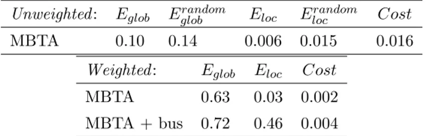
1.3.7 Efficiency and cost of real-world networks . . . 41
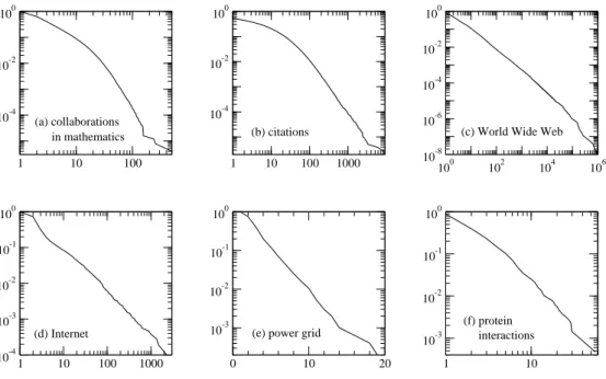
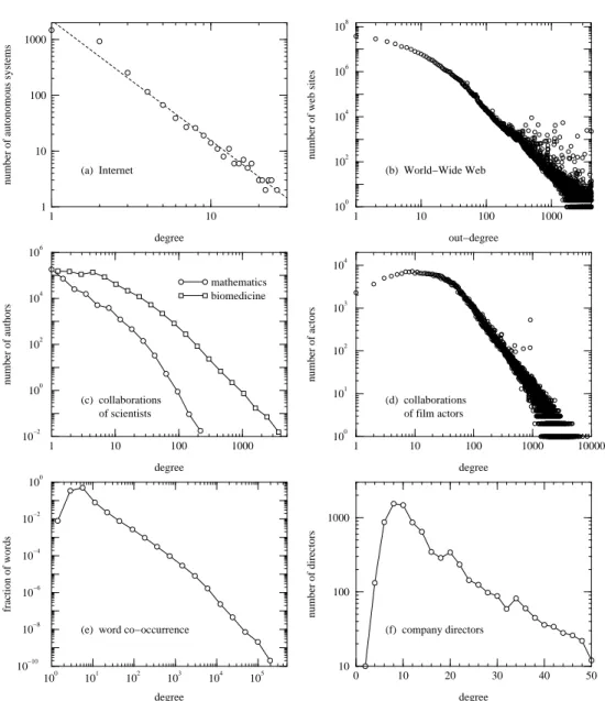
1.3.8 Degree distributions . . . 52
1.3.9 Network resilience . . . 55
1.3.10 Network navigation . . . 58
1.4 Random graphs . . . 59
1.5 Scale-free networks . . . 67
1.6 A simulation tool for the analysis of complex networks . . . 70
1.7 Conclusions . . . 78
2 Identification of complex networks by the method of stages 81 2.1 Introduction . . . 82
2.2 Description of the network properties that will be computed in
simulations . . . 84
2.3 Distribution fitting with the method of stages . . . 86
2.4 Case study: experimental results . . . 91
2.5 Conclusions . . . 99
3 Tracking control with time delay compensation for linear time invariant networked control systems 101 3.1 Introduction . . . 102
3.2 Problem statement and solution . . . 103
3.3 Numerical results . . . 111
Introduction to complex
networks
This chapter aims to provide an overview on complex networks, trying to in-vestigate what apparently different kinds of networks have in common. Sys-tems belonging to different branches of science, such as metabolic pathways and ecosystems, the Internet and propagation of HIV infection share similar network architectures. Many systems in the real-world can be modeled as net-works. For example, the patterns of connections between economic agents form a social network, since often partners are chosen not on economic grounds but for social reasons. It is clear that the structure of such networks affects the pattern of economic transactions. In the last years, researchers have con-ducted extensive investigations of networks in economics, mathematics, soci-ology and several other fields, trying to understand and explain network effects [93]. Inspired by empirical studies of networked control systems such as the Internet, social networks and biological networks, researchers have developed a variety of techniques and models to help us understand or predict the be-havior of these systems [92]. The content of this chapter is mainly based on [12, 20, 74, 91, 92, 95, 126]. My research results are presented in Sec. 1.6, Chap. 2 and Chap. 3.
1.1
Introduction
A network is a set of items, called vertices or sometimes nodes, with connec-tions between them, called edges (Fig. 1.1). Examples of systems taking the
edge vertex
Figure 1.1: A small example network with eight vertices and ten edges [92]. form of networks (also called graphs in much of the mathematical literature) are ubiquitous in the real-world: the Internet, the World Wide Web, social networks of acquaintance or other connections between individuals, neural net-works, metabolic netnet-works, food webs, networks of citations between papers, etc (Fig. 1.2).
The first proof in theory of networks is probably the Euler’s solution of the Kon¨ıgsberg bridge problem. Networks have been studied extensively in the social sciences: in particular, typical social network studies address issues of centrality (which individuals are best connected to others or have most influence) and connectivity (wether and how individuals are connected to one another through the network).
Recently, thanks to the availability of computers and communication net-works, the focus of network research is shifting away from the analysis of single small graphs and the properties of individual vertices or edges within such graphs to consideration of large-scale statistical properties of graphs. This change of scale implies a corresponding change in our analytic approach. For example, with reference to a network containing millions of vertices, it has little meaning asking which vertex would prove most crucial to the net-work connectivity if it were removed. On the other hand, it is meaningful asking what percentage of vertices need to be removed to substantially affect
(c) (b)
(a)
Figure 1.2: Three examples of real-world networks. (a) A visualization of the network structure of the Internet at the level of “autonomous systems” – local groups of computers each representing hundreds or thousands of machines. Picture by Hal Burch and Bill Cheswick (b) A social network, in this case of sexual contacts, redrawn from the HIV data of Potterat et al. [101]. (c) A food web of predator-prey interactions between species in a freshwater lake [81].
network connectivity. Moreover, the analysis of large networks must necessar-ily abstract from their graphical representation: the role played in the past by the human eye is now played by the statistical methods, which permit to investigate the structure and properties of very large networks. In fact, for networks of tens or hundreds of vertices, it is a relatively straightforward matter to draw a picture of the network with actual points and lines, and to answer specific questions about network structure by examining this picture. This has been one of the primary methods of network analysts since the field began (Fig. 1.3). The human eye is an analytic tool of remarkable power, and
Figure 1.3: An early hand-drawn social network from 1934 representing friend-ships between school children. After Moreno [85].
eyeballing pictures of networks is an excellent way to gain an understanding of their structure. With a network of a million or a billion vertices, however, this approach is useless. (Fig. 1.2a shows an example of a network that lies at the upper limit of what can usefully be drawn on a piece of paper or computer screen.)
Researchers have got important results on the characterization and mod-eling of network structure, while a lot of work still remains to do for under-standing the effects of structure on system behavior.
A network can be mathematically represented by a graph [116] in which vertices represent systems and edges represent the relationships between them. There can be more than one type of vertex or edge and vertices or edges may
have a variety of properties associated with them. Graphs can be weighted or unweighted, directed or undirected; directed graphs (or digraphs, for short) can be cyclic or acyclic, etc (Fig. 1.4). Graphs containing hyperedges (edges
(b)
(d) (a)
(c)
Figure 1.4: Examples of various types of networks [92]: (a) an undirected network with only a single type of vertex and a single type of edge; (b) a network with a number of discrete vertex and edge types; (c) a network with varying vertex and edge weights; (d) a directed network in which each edge has a direction.
joining more than two vertices together) are called hypergraphs. Graphs that contain vertices of two distinct types, with edges running only between unlike types, are called bipartite graphs (Fig. 1.5). An example of bipartite graph are the affiliation (or collaboration) networks, in which people are joined together by common membership of groups, the two types of vertices representing the people and the groups. An example of such networks is the network of col-laborations of movie actors: in this case, the two types of vertices are movies and actors, and the network can be represented as a graph with edges run-ning between each movie and the actors that appear in it. Researchers have also considered the projection of this graph onto the unipartite space of actors only, also called a one-mode network [123] (Fig. 1.5). In such a projection two actors are considered connected if they have appeared in a movie together. The construction of the one-mode network however involves discarding some
B D A C E F G H I J K A B C D E F G H I J K 1 2 3 4
Figure 1.5: A schematic representation (top) of a bipartite graph, such as the graph of movies and the actors who have appeared in them. In this small graph there are four movies, labeled 1 to 4, and eleven actors, labeled A to K, with edges joining each movie to the actors in its cast. The lower part of the picture shows the one-mode projection of the graph for the eleven actors [95]. of the information contained in the original bipartite network, and for this reason it is more desirable to model collaboration networks using the full bi-partite structure. Moreover, graphs may evolve over time, with vertices or edges appearing or disappearing, or values defined on those vertices and edges changing.
The jargon of the study of networks is unfortunately confused by differing usages among investigators from different fields. To avoid (or at least reduce) confusion, a short glossary of terms as they are used in this thesis is provided:
• Vertex (pl. vertices): The fundamental unit of a network, also called a
site (physics), a node (computer science), or an actor (sociology).
• Edge: The line connecting two vertices. Also called a bond (physics), a
link (computer science), or a tie (sociology).
(such as a one-way road between two points), and undirected if it runs in both directions. Directed edges, which are sometimes called arcs, can be thought of as sporting arrows indicating their orientation. A graph is directed if all of its edges are directed. An undirected graph can be represented by a directed one having two edges between each pair of connected vertices, one in each direction.
• Degree: The number of edges connected to a vertex. Note that the
degree is not necessarily equal to the number of vertices adjacent to a vertex, since there may be more than one edge between any two vertices. In a few recent articles, the degree is referred to as the “connectivity” of a vertex, but here this usage is avoided because the word connectivity already has another meaning in graph theory. A directed graph has both an in-degree and an out-degree for each vertex, which are the numbers of incoming and outgoing edges respectively.
• Component: The component to which a vertex belongs is that set of
vertices that can be reached from it by paths running along edges of the graph. In a directed graph a vertex has both an in-component and an out-component, which are the sets of vertices from which the vertex can be reached and which can be reached from it.
• Geodesic path: A geodesic path is the shortest path through the network
from one vertex to another. Note that there may be and often is more than one geodesic path between two vertices.
• Diameter: The diameter of a network is the length (in number of edges)
of the longest geodesic path between any two vertices. A few authors have also used this term to mean the average geodesic distance in a graph, although strictly the two quantities are quite distinct.
1.2
Real-world networks
A social network is a set of people or groups of people with some pattern of contacts or interactions between them [107, 123] (Fig. 1.2b). The first theorist to stress the importance of the degree distribution (i.e., the probability with which a vertex has a certain number of edges connected to it) in networks of all kinds was probably Anatol Rapoport [102], whose mathematical models are of particular note. Another important set of experiments are the famous “small-world” experiments of Milgram [82, 119], which probed the distribution of path lengths in an acquaintance network by asking participants to pass a letter to one of their first-name acquaintances in an attempt to get it to an assigned target individual. Most of the letters in the experiment were lost, but about a quarter reached the target and passed on average through the hands of only about six people in doing so. This experiment was the origin of the popular concept of the “six degrees of separation”, although that phrase did not appear in Milgram’s writing, being coined some decades later by Guare [54].
Traditional social network studies often suffer from problems of inaccu-racy, subjectivity and small sample size. Because of these problems, many researchers have turned to other methods for probing social networks. One source of copious and relatively reliable data is collaboration networks. These are typically affiliation networks in which participants collaborate in groups of one kind or another and links between pairs of individuals are established by common group membership. Examples of such networks are the collab-oration network of film actors, networks of company directors, networks of coauthorship among academics, etc.
The classic example of an information network is the network of citations between academic papers [44]. These citations form a network in which the vertices are articles and a directed edge from article A to article B indicates that A cites B (Fig. 1.6). Citation networks are acyclic because papers can only cite other papers that have already been written, not those that have yet
World−Wide Web citation network
Figure 1.6: The two best studied information networks [92]. Left: the citation network of academic papers in which the vertices are papers and the directed edges are citations of one paper by another. Since papers can only cite those that came before them (lower down in the figure) the graph is acyclic – it has no closed loops. Right: the World Wide Web, a network of text pages accessible over the Internet, in which the vertices are pages and the directed edges are hyperlinks. There are no constraints on the Web that forbid cycles and hence it is in general cyclic.
to be written. In 1926 Alfred Lotka discovered the so-called Law of Scientific Productivity, which states that the distribution of the numbers of papers writ-ten by individual scientists follows a power law: the number of scientists who have written k papers falls off as k−α for some constant α. An interesting
de-velopment in the study of citation patterns has been the arrival of automatic citation “crawlers” that construct citation networks from online papers.
Another important example of an information network is the World Wide Web, which is a network of Web pages containing information, linked together by hyperlinks from one page to another [56] (Fig. 1.6). The Web should not be confused with the Internet, which is a physical network of computers linked together by optical fibre and other data connections. Unlike a citation network, the World Wide Web is cyclic: there is no natural ordering of sites and no constraints that prevent the appearance of closed loops. The Web is a directed network and appears to have power-law distributions for both in-and out-degree. Data about the Web come from “crawls” of the network, in which Web pages are found by following hyperlinks from other pages [24]. The obtained picture of the network structure of the World Wide Web is therefore necessarily biased: crawls usually cover only a part of the Web, thus pages are more likely to be found the more other pages point to them [76].
Preference networks provide an example of a bipartite information network. A preference network is a network with two kinds of vertices representing individuals and the objects of their preference, such as books or films, with an edge connecting each individual to the books or films they like. Preference networks can be weighted to indicate strength of likes or dislikes and can also be thought of as social networks, linking not only people to objects, but also people to other people with similar preferences. Networks of this kind form the basis for collaborative filtering algorithms and recommender systems, which are techniques for predicting new likes or dislikes based on comparison of individuals’ preferences with those of others. Collaborative filtering has found considerable commercial success for product recommendation and targeted
advertising particularly with online retailers.
Technological networks are man-made networks designed typically for dis-tribution of some commodity or resource, such as electricity or information. Examples of distribution networks are the electric power grid [14, 124, 126], the network of airline routes [14], and networks of roads [64], railways [73, 109] and pedestrian traffic [28].
Another widely studied technological network is the Internet, i.e., the net-work of physical connections between computers. Since there is a large and ever-changing number of computers on the Internet, the structure of the net-work is usually examined at a coarse-grained level, either the level of routers, special-purpose computers on the network that control the movement of data, or autonomous systems, which are groups of computers within which network-ing is handled locally, but between which data flows over the public Internet (Fig. 1.2a). Traceroute programs can report the sequence of network nodes that a data packet passes through when traveling between two points and are therefore used to reconstruct the physical structure of the network.
The classic example of a biological network is probably the network of metabolic pathways, which is a representation of metabolic substrates and products with directed edges joining them if a known metabolic reaction ex-ists that acts on a given substrate and produces a given product. A separate network is the network of mechanistic physical interactions between proteins (as opposed to chemical reactions among metabolites), which is usually re-ferred to as a protein interaction network.
Another example of a biological network is the food web (Fig. 1.2c), in which the vertices represent species in an ecosystem and a directed edge from species A to species B indicates that A preys on B. Sometimes the relationship is drawn the other way around, because ecologists tend to think in terms of energy or carbon flows through food webs; a predator-prey interaction is thus drawn as an arrow pointing from prey to predator, indicating energy flow from prey to predator when the prey is eaten. Neural networks, blood vessels and
the equivalent vascular networks in plants are other examples of biological networks.
1.3
Properties of networks
The famous experiments carried out by Stanley Milgram in the 1960s, de-scribed in Sec. 1.2, are one of the first direct demonstrations of the small-world effect, the fact that most pairs of vertices in most networks seem to be con-nected by a short path through the network. The existence of the small-world effect had been speculated upon before Milgram’s work, notably in a remark-able 1929 short story by the Hungarian writer Frigyes Karinthy [65] and more rigorously in the mathematical work of Pool and Kochen [36] which, although published after Milgram’s studies, was in circulation in preprint form for a decade before Milgram took up the problem.
1.3.1 Characteristic path length and clustering coefficient
For an undirected and unweighted (topological) network, the average distance between vertex pairs (characteristic path length) is defined as [72, 74]
L = 1 N (N − 1)
X
i6=j
dij,
where N is the number of nodes and dij is the geodesic (shortest) distance
from vertex i to vertex j. In other words, L is the number of edges in the shortest path between two vertices, averaged over all pairs of vertices. It has been shown that many real-world networks exhibit small values of L, much smaller than the number N of vertices.
If the graph is not connected, there exist vertex pairs that have no connect-ing path or, equivalently, whose geodesic distance is infinite and, accordconnect-ingly, L becomes infinite. To avoid this problem, L is usually defined on such networks to be the mean geodesic distance between all pairs that have a connecting
path. Pairs that fall in two different components (maximal subsets of ver-tices that are connected by paths through the network) are excluded from the average.
The small-world effect has obvious implications for the dynamics of pro-cesses taking place on networks, as for example the spread of information across a network, and also underlies some well-known parlor games, particu-larly the calculation of Erd˝os numbers [35] and Bacon numbers.
On the other hand, the small-world effect is also mathematically obvious: in fact, if the number n of vertices within a distance r of a typical central vertex grows exponentially with r – and this is true of many networks, including the random graph – then the value of L will increase as ln N :
n ∝ eαr ⇒ N ∝ eαd2 ⇒ d ∝ ln N ⇒ L ∝ ln N ,
where α is a positive real constant and d is the diameter of the network, that is, the length (in number of edges) of the longest geodesic path between any two vertices. Networks are said to show the small-world effect if the value of L scales logarithmically or slower with network size for fixed mean degree [92]. Logarithmic scaling has been observed in various real-world networks [9, 88, 89].
In many networks it is found that if vertex A is connected to vertex B and vertex B to vertex C, then there is a heightened probability that vertex A will also be connected to vertex C. In the language of social networks, the friend of your friend is likely also to be your friend. This property is called network transitivity. In terms of network topology, transitivity means the presence of a heightened number of triangles in the network – sets of three vertices each of which is connected to each of the others. It can be quantified by defining a clustering coefficient C thus:
C = 3 × number of triangles in the network
number of connected triples of vertices, (1.1)
where a “connected triple” means a single vertex with edges running to an unordered pair of others (Fig. 1.7). In effect, C measures the fraction of
triples that have their third edge filled in to complete the triangle. The factor of three in the numerator accounts for the fact that each triangle contributes to three triples and ensures that C lies in the range 0 ≤ C ≤ 1. In simple terms, C is the mean probability that two vertices that are network neighbors of the same other vertex will themselves be neighbors.
An alternative definition of the clustering coefficient has been given by Watts and Strogatz [126], who proposed defining a local value
Ci = number of triangles connected to vertex inumber of triples centered on vertex i . (1.2)
For vertices with degree 0 or 1, for which both numerator and denominator are zero, Ci:= 0. The clustering coefficient for the whole network is the average
C = 1 N
X
i
Ci. (1.3)
The quantities in (1.2) and (1.3) can also be computed in the following way. If the generic vertex i has ki neighbors, then at most ki(ki− 1)/2 edges can
exist between them (this occurs when every neighbor of i is connected to every other neighbor of i); Ci is the fraction of these allowable edges that actually exist and C is the average of Ci over all i. Fig. 1.7 illustrates the difference
Figure 1.7: Illustration of the definition of the clustering coefficient C (1.1) [92]. This network has one triangle and eight connected triples, and therefore has a clustering coefficient of 3 × 1/8 = 38. The individual vertices have local clustering coefficients (1.2) of 1, 1, 1
6, 0 and 0, for a mean value (1.3) of
C = 1330.
The clustering coefficient measures the density of triangles in a network. An obvious generalization is to ask about the density of longer loops also: loops of length four and above. If more than one edge is permitted between a pair of vertices, then there is also a lower order clustering coefficient that describes the density of loops of length two. This coefficient is particularly important in directed graphs where the two edges in question can point in opposite directions. The probability that two vertices in a directed network point to each other is called the reciprocity and is often measured in directed social networks [107, 123].
1.3.2 Networks between regularity and randomness
Ordinarily, the connection topology of several network models is assumed to be either completely regular or completely random. But many biological, techno-logical and social networks lie somewhere between these two extremes. In [126], the authors explore simple models of networks that can be tuned through this middle ground: regular networks ‘rewired’ to introduce increasing amounts of disorder. They find that these systems can be highly clustered, like reg-ular lattices, yet have small characteristic path lengths, like random graphs. They call them ‘small-world’ networks, by analogy with the small-world phe-nomenon [54, 70, 82]. The neural network of the worm Caenorhabditis elegans, the power grid of the western United States and the collaboration graph of film actors are examples of small-world networks.
To interpolate between regular and random networks, the following random rewiring procedure is considered (Fig. 1.8). Starting from a ring lattice with N vertices and k edges per vertex, each edge is randomly rewired with probability
p. This construction allow to ‘tune’ the graph between regularity (p = 0) and
disorder (p = 1), and thereby to probe the intermediate region 0 < p < 1 , about which little is known. A vertex and the edge that connects it to its nearest neighbor are chosen in a clockwise sense. The edge is reconnected with probability p to a vertex chosen uniformly at random over the entire
p = 0 p = 1 Increasing randomness
Regular Small-world Random
Figure 1.8: Random rewiring procedure for interpolating between a regular ring lattice and a random network, without altering the number of vertices or edges in the graph (N = 20, k = 4) [126].
ring, with duplicate edges forbidden; otherwise the edge is left in place. This process is repeated by moving clockwise around the ring, considering each vertex in turn until one lap is completed. Next, the edges that connect vertices to their second-nearest neighbors are considered clockwise. As before, each of these edges is randomly rewired with probability p, and this process continues, circulating around the ring and proceeding outwards to more distant neighbors after each lap, until each edge in the original lattice has been considered once. (As there are N k/2 edges in the entire graph, the rewiring process stops after
k/2 laps.)
Three realizations of this process are shown in Fig. 1.8, for different values of p. For p = 0, the original ring is unchanged; as p increases, the graph be-comes increasingly disordered until for p = 1 all edges are rewired randomly. For intermediate values of p, the graph is a small-world network: highly clus-tered like a regular graph, yet with small characteristic path length, like a random graph (Fig. 1.9). The structural properties of these graphs are quan-tified by their characteristic path length L(p) and clustering coefficient C(p). In particular, L(p) measures the typical separation between two vertices in the graph (a global property), whereas C(p) measures the cliquishness of a typical neighborhood (a local property). The considered networks have many vertices with sparse connections, but not so sparse that the graph is in danger of
be-0 0.2 0.4 0.6 0.8 1 0.0001 0.001 0.01 0.1 1 p L(p) / L(0) C(p) / C(0)
Figure 1.9: Characteristic path length L(p) and clustering coefficient C(p) for the family of randomly rewired graphs described in Fig. 1.8 [126].
coming disconnected. Specifically, the authors require N À k À ln N À 1, where k À ln N guarantees that a random graph will be connected [23]. In this regime, it is found that L ∼ N/2k À 1 and C ∼ 3/4 as p → 0, while
L ≈ Lrandom ∼ ln N/ ln k and C ≈ Crandom ∼ k/N ¿ 1 as p → 1. Thus
the regular lattice at p = 0 is a highly clustered, large world where L grows linearly with N , whereas the random network at p = 1 is a poorly clustered, small world where L grows only logarithmically with N . These limiting cases might lead one to suspect that large C is always associated with large L, and small C with small L. On the contrary, Fig. 1.9 reveals that there is a broad in-terval of p over which L(p) is almost as small as Lrandom yet C(p) À Crandom. These small-world networks result from the immediate drop in L(p) caused by the introduction of a few long-range edges. Such ‘short cuts’ connect ver-tices that would otherwise be much farther apart than Lrandom. For small p,
each short cut has a highly nonlinear effect on L, contracting the distance not just between the pair of vertices that it connects, but between their immedi-ate neighborhoods, neighborhoods of neighborhoods and so on. By contrast, an edge removed from a clustered neighborhood to make a short cut has, at most, a linear effect on C; hence C(p) remains practically unchanged for small
p even though L(p) drops rapidly. The important implication here is that at
undetectable. To check the robustness of these results, the authors have tested many different types of initial regular graphs, as well as different algorithms for random rewiring, and all give qualitatively similar results. The only re-quirement is that the rewired edges must typically connect vertices that would otherwise be much farther apart than Lrandom.
The idealized construction above reveals the key role of short cuts. It sug-gests that the small-world phenomenon might be common in sparse networks with many vertices, as even a tiny fraction of short cuts would suffice. To test this idea, the authors computed L and C for the collaboration graph of actors in feature films, the electrical power grid of the western United States and the neural network of the nematode worm Caenorhabditis elegans [1]. All three graphs are of scientific interest. The graph of film actors is a surrogate for a social network [123], with the advantage of being much more easily specified. It is also akin to the graph of mathematical collaborations centered, tradition-ally, on P. Erd˝os. The graph of the power grid is relevant to the efficiency and robustness of power networks [99] and C. elegans is the sole example of a completely mapped neural network.
For friendship networks, the characteristic path length and the clustering coefficient have intuitive meanings: L is the average number of friendships in the shortest chain connecting two people; Ci reflects the extent to which
friends of i are also friends of each other; and thus C measures the cliquishness of a typical friendship circle. The data shown in Fig. 1.9 are averages over 20 random realizations of the rewiring process described in Fig. 1.8, and have been normalized by the values L(0), C(0) for a regular lattice. All the graphs have N = 1000 vertices and an average degree of k = 10 edges per vertex. A logarithmic horizontal scale has been used to resolve the rapid drop in L(p), corresponding to the onset of the small-world phenomenon. During this drop,
C(p) remains almost constant at its value for the regular lattice, indicating
that the transition to a small world is almost undetectable at the local level. The graphs considered in Table 1.1 are defined as follows [126]. Two actors
Table 1.1: Empirical examples of small-world networks [126].
Lactual Lrandom Cactual Crandom
Film actors 3.65 2.99 0.79 0.00027
Power grid 18.7 12.4 0.080 0.005
C. elegans 2.65 2.25 0.28 0.05
are joined by an edge if they have acted in a film together. The attention is restricted to the giant connected component [23] of this graph, which includes
∼ 90% of all actors listed in the Internet Movie Database, as of April 1997.
For the power grid, vertices represent generators, transformers and substa-tions, and edges represent high voltage transmission lines between them. For C. elegans, an edge joins two neurons if they are connected by either a synapse or a gap junction. All edges are treated as undirected and unweighted, and all vertices as identical, though these are crude approximations. All three networks show the small-world phenomenon: L & Lrandom but C À Crandom.
These examples were not hand-picked; they were chosen because of their in-herent interest and because complete wiring diagrams were available. Thus the small-world phenomenon is not merely a curiosity of social networks nor an artefact of an idealized model – it is probably generic for many large, sparse networks found in nature.
In [126] the functional significance of small-world connectivity for dynam-ical systems is also investigated. The considered test case is a deliberately simplified model for the spread of an infectious disease. The population struc-ture is modeled by the family of graphs described in Fig. 1.8. At time t = 0, a single infective individual is introduced into an otherwise healthy population. Infective individuals are removed permanently (by immunity or death) after a period of sickness that lasts one unit of dimensionless time. During this time, each infective individual can infect each of its healthy neighbors with probability r. On subsequent time steps, the disease spreads along the edges of the graph until it either infects the entire population, or it dies out, having
infected some fraction of the population in the process.
Two results emerge. First, the critical infectiousness rhalf, at which the
disease infects half the population, decreases rapidly for small p (Fig. 1.10a). Second, for a disease that is sufficiently infectious to infect the entire
popu-0.15 0.2 0.25 0.3 0.35 0.0001 0.001 0.01 0.1 1 r half p a 0 0.2 0.4 0.6 0.8 1 0.0001 0.001 0.01 0.1 1 T(p) /T(0) L(p) /L(0) p b
Figure 1.10: The community structure is given by one realization of the family of randomly rewired graphs used in in Fig. 1.8. a, Critical infectiousness
rhalf, at which the disease infects half the population, decreases with p. b,
The time T (p) required for a maximally infectious disease (r = 1) to spread throughout the entire population has essentially the same functional form as the characteristic path length L(p). Even if only a few per cent of the edges in the original lattice are randomly rewired, the time to global infection is nearly as short as for a random graph [126].
lation regardless of its structure, the time T (p) required for global infection resembles the L(p) curve (Fig. 1.10b). Thus, infectious diseases are predicted to spread much more easily and quickly in a small world; the alarming and
less obvious point is how few short cuts are needed to make the world small.
1.3.3 Global and local efficiency
The approach of Watts and Strogatz described in Sec. 1.3.2 can be used when the only information retained of a real network is about the existence or the absence of a link, nothing is known about the physical length of the link (or more generically the weight associated with the link, i.e., the graph is unweighted) and multiple edges between the same couple of nodes are not allowed (i.e., the graph is simple). Moreover, the assumption of connectedness is necessary because otherwise the quantity L would diverge.
Of course, a generalization of the approach of Watts and Strogatz to weighted networks would allow a more detailed analysis of real networks and would extend the range of applications. For example, with reference to the same three real networks studied in [126], the analysis of the network of film actors must be restrained to only a part of the system, the giant connected component of the graph, in order to avoid the divergence of L. Moreover, the topological approximation only provides whether actors participated in some movie together or if they did not at all. In reality there are, instead, various degrees of correlation: two actors that have done ten movies together are in a much stricter relation than two actors that have acted together only once. It is possible to better shape this different degree of friendship by us-ing a non-simple graph or by usus-ing a weighted network: if two actors have acted together, a weight is associated with their connection by saying that the length of the connection, instead of being always equal to one, is equal to the inverse of the number of movies they did together. In the case of the neural network of the C. elegans, Watts and Strogatz define an edge in the graph when two vertices are connected by either a synapse or a gap junction. This is only a first approximation of the real network. Neurons are different one from the other and some of them are in much stricter relation than others: the number of junctions connecting a couple of neurons can vary a lot, up to
a maximum of 72 in the case of the C. elegans. As in the case of film actors, a weighted network is more suited to describe such a system and can be de-fined by setting the length of the connection i − j as equal to the minimum between 1 and the inverse of the number of junctions between i and j. The last network studied in [126], the electrical power grid of the western United States, is clearly a network where the geographical distances play a fundamen-tal role. Any of the high voltage transmission lines connecting two stations of the network has a length, and the topological approximation, which neglects such lengths, is a poor description of the system. Of course, a generalization of the analysis to weighted networks would also extend the application of the small-world concept to a realm of new networks. A very significative exam-ple is that of transportation system: public transportation (bus, subway and trains), highways, airplane connections.
In [74] the authors present a way to extend the small-world analysis from topological to weighted networks. A weighted network can be characterized by introducing the variable efficiency E, which measures how efficiently the nodes exchange information. The definition of small-world behavior can be formu-lated in terms of the efficiency: this single measure evaluated on a global and on a local scale plays in turn the role of L and C. Small-world networks result as systems that are both globally and locally efficient [72]. The formalism is valid both for weighted and unweighted (topological) networks. In the case of topological networks, the measures introduced in [74] do not coincide ex-actly with those given by Watts and Strogatz. For example, the measures introduced in [74] also work in the case of unconnected graphs. An impor-tant quantity, previously not considered, is the cost of a network. Often high (global and local) efficiency implies a high cost of the network.
A weighted and possibly even non-connected and non-sparse graph is con-sidered. A weighted graph needs two matrices to be described:
• The adjacency matrix [aij], containing the information about the
as a set of numbers aij = 1 when there is an edge joining i to j, and
aij = 0 otherwise;
• A matrix of the weights associated with each link. This matrix [wij]
is named the matrix of physical distances because the number wij can be imagined as the space distance between i and j. Moreover, wij is
assumed to be known even if in the graph there is no edge between i and
j.
To make a few concrete examples: wij can be identified with the geograph-ical distance between stations i and j both in the case of the electrgeograph-ical power grid of the western United States studied by Watts and Strogatz and in the case of other transportation systems considered in [74]. In such a situation
wij satisfy the triangular inequality, though in general this is not a necessary
assumption. The presence of multiple edges, typical of the neural network of the C. elegans and of social systems like the network of film actors, can be included in the same framework by setting wij equal to the minimum between 1 and the inverse of the number of edges between i and j (respectively, the inverse of the number of junctions between two neurons or the inverse of the number of movies two actors did together). This allows to remove the hypoth-esis of simple network and to consider also non-simple systems as weighted networks. The resulting weighted network is, of course, a case in which the triangular inequality is not satisfied. For a computer network or Internet, wij
can be assumed to be proportional to the time needed to exchange a unitary packet of information between i and j through a direct link. Or as 1/vij,
the inverse of the velocity of a chemical reaction along a direct connection in a metabolic network. Of course, in the particular case of an unweighted (topological) graph wij = 1 ∀ i 6= j.
In a weighted graph the definition of the shortest path length dij between two generic points i and j is different from the definition used for an unweighted graph. In this case the shortest path length dij is in fact defined as the smallest
from i to j. Again, when wij = 1 ∀ i 6= j, i.e., in the particular case of an
unweighted graph, dij reduces to the minimum number of edges traversed to
get from i to j. The matrix of the shortest path lengths [dij] is therefore
calculated by using the information contained both in matrix [aij] and in matrix [wij] (for example, by using Dijkstra’s algorithm (O(N2log N )). It is
supposed that every vertex sends information along the network through its edges and that the efficiency ²ij in the communication between vertices i and
j is inversely proportional to the shortest distance: ²ij = 1/dij ∀ i, j. This is a
reasonable approximation in general, but sometimes other relationships might be used, especially when justified by a more specific knowledge about the system. By assuming ²ij = 1/dij, when there is no path in the graph between
i and j the shortest path length between them is dij = ∞ and consistently
²ij = 0. Consequently, the average efficiency of the graph can be defined as
[112] E = P i6=j²ij N (N − 1) = 1 N (N − 1) X i6=j 1 dij . (1.4)
If the graph is undirected, i.e., there is no associated direction with the links, both [wij] and [dij] are symmetric matrices and therefore the quantity E can be defined simply by using only half of the matrix as
E = 2 N (N − 1) X i<j 1 dij .
Anyway the more general definition (1.4) allows to easily apply the presented formalism to directed graphs as well.
Formula (1.4) gives a value of E that can vary in the range [0, ∞]. It would be more practical to have E normalized to be in the interval [0, 1]. E can be normalized by considering the ideal case in which the graph has all the N (N − 1)/2 possible edges. In such a case the information is propagated in the most efficient way and E assumes its maximum value. The efficiency
E considered in the following is always normalized: 0 ≤ E ≤ 1. Though the
each couple of vertices (in networks in which the triangular inequality holds), real networks can nevertheless assume high values of E.
One of the advantages of the efficiency-based formalism is that a single measure, the efficiency E (instead of the two different measures L and C used in the Watts Strogatz (WS) formalism) is sufficient to define the small-world behavior. In fact, on one hand, the quantity defined in (1.4) can be evaluated as it is for the whole graph to characterize the global efficiency of the graph; in this case, it is denoted by Eglob. Being the efficiency in communication
between two generic vertices, Eglob plays a role similar to the inverse of the characteristic path length L. In fact, L is the mean of dij, while Eglob is the
average of 1/dij, i.e., the inverse of the harmonic mean of [dij]. Nowadays the
harmonic mean finds extensive applications in a variety of different fields: in particular it is used to calculate the average performance of computer systems [86, 112], parallel processors [57] and communication devices (for example, modems and Ethernets [59]). In all such cases, where a mean flow-rate of information has to be computed, the simple arithmetic mean gives the wrong result. In some cases 1/L gives a good approximation of Eglob, although Eglob
is the real variable to be considered to characterize the efficiency of a system transporting information in parallel. In the particular case of a disconnected graph the difference between the two quantities is evident because L = ∞ while Eglob is a finite number.
On the other hand the same measure, the efficiency, can be evaluated for any subgraph of the graph and therefore it can be used also to characterize the local properties of the graph itself. In the WS formalism it is not possible to use the characteristic path length for quantifying both the global and the local properties of the graph simply because L cannot be calculated locally, most of the subgraphs of the neighbors of a generic vertex i being disconnected. Since E is defined also for a disconnected graph, it is possible to characterize the local properties of the graph by evaluating for each vertex i the efficiency of the subgraph of the neighbors of i. The local efficiency Eloc is defined as
the average of the N values obtained in this way. Here, for each vertex i, the normalization factor is the the efficiency of the ideal case in which the subgraph has all the ki(ki− 1)/2 possible edges, where ki is the number of neighbors of
vertex i. Elocplays a role similar to the clustering coefficient C: since vertex
i does not belong to the relative subgraph, the local efficiency Eloc tells how
much the system is fault tolerant, thus how efficient is the communication between the first neighbors of i when i is removed. This concept of fault tolerance is different from that adopted in [11, 29, 33], where the authors consider the response of the entire network to the removal of a node i. Here the response of the subgraph of first neighbors of i to the removal of i is considered.
A new, generalizing, definition of small world can be introduced, built in terms of the characteristics of information flow at global and local level: a small-world network is a network with high Eglob and Eloc, i.e., very efficient
both in global and local communication [74]. This definition is valid both for unweighted and for weighted graphs, and can also be applied to disconnected graphs and/or non-sparse graphs.
1.3.4 Comparison between Eglob, Eloc and L, C
In [74] the authors also study the correspondence between their measures and the quantities L and C defined in [126] (or, correspondingly, 1/L and C). The fundamental difference is that 1/L measures the efficiency of a sequential system, that is to say, of a system where there is only one packet of information going along the network. On the other hand, Eglob measures the efficiency for parallel systems, where all the nodes in the network concurrently exchange packets of information. This can explain why L works reasonably: it can be seen that 1/L is a reasonable approximation of Eglob when there are not huge differences among the distances in the graph, and so considering just one packet in the system is more or less equivalent to the case where multiple packets are present. This is the case for all the networks presented in [126],
and this effect is strengthened even more by the fact that the topology only is considered.
Having explained why L behaves relatively well in some case, it is also worth noticing that, like every approximation, it fails to properly deal with all cases. For example, the sequentiality of the measure 1/L explains why many limitations have to be introduced, like connectedness, that are present just in order to make the formulas valid. Consider the limit case where a node is isolated from the system. In the case of a neural network, this corresponds for example to the death of a neuron. In this case, 1/L drops to zero (L = ∞), which is of course not the overall efficiency of the system: in fact, the brain continues to work, as all the other neurons continue to exchange information; only, the efficiency is just slightly diminished, as now there is one neuron less and, correctly, this is properly taken into account using Eglob.
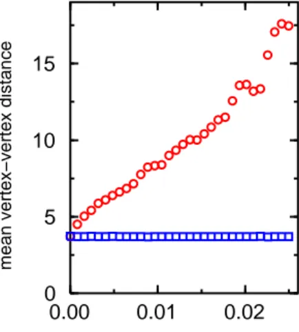
Even without dropping the connectedness assumption, another example can show how in the limit case, the approximation given by 1/L diverges from the real efficiency measure. Fig. 1.11 shows the addition of a new node to the Internet (which already had N nodes), with efficiency ε, that can be seen as the speed of the connection. This happens every time the Internet is augmented with a new computer and every time a computer is turned on. A situation like this occurs daily in the order of the millions. How does it globally affect the Internet, according to L and Eglob? It can be proved that
L augments by approximately 1
ε(N +1). This means that if for any reason, the
connection speed is particularly slow (or becomes such, for example due to a congestion, or the computer gets low in resources), L of the whole Internet is heavily affected and can rapidly become enormous. Even, whenever the computer blocks (or it is shut down), L diverges to infinity (like, so to say, if the Internet had collapsed). On the other hand, the efficiency Eglobhas a relative decrement of approximately N +12 , which means that in practice, as N is quite large, the particular behavior of the new computer affects the Internet in a negligible way. Summing up, having one or few computers with an extremely
Figure 1.11: A new computer is attached to the Internet (which already had
N nodes) with a connection represented by a small efficiency ε. Having one
(or few) computer with an extremely slow connection, does not mean that the whole Internet diminishes by far its efficiency: in practice, the presence of such slow computer goes unnoticed, because the other thousands of computers are exchanging packets among them in a very efficient way. L fails to properly capture the global behavior of systems like the Internet, unlike Eglob, that perfectly matches the observed behavior [74].
slow connection, does not mean that the whole Internet diminishes by far its efficiency: in practice, the presence of such few very slow computers goes unnoticed, because the other thousands of computers are exchanging packets among them in a very efficient way. Therefore, L fails to properly capture the global behavior of systems like the Internet (1/L would give a number very close to zero, because it measures the average efficiency in case a single packet is active through the Internet), unlike Eglob, that perfectly matches the
observed behavior.
The crucial point here is the following: all the networks considered in [126] to justify the definition of small worlds (and, in fact, most of the networks that model complex systems) are parallel systems, where all the nodes interact in parallel (Internet, World Wide Web, social networks, neural systems and so on). With this assumption, Eglob measures the real efficiency of the system, and 1/L is just a first rough approximation, as it deals with the sequential case only. As for C and Eloc, it can be shown that C, in the case of undirected topological graphs, is always a reasonable approximation of Eloc. Therefore,
the seemingly ad hoc nature of C in the WS formalism now finds a new meaning in the general notion of efficiency. There are not two different kinds of properties to consider when analyzing a network on the local and on the global scale, but just one unifying concept: the efficiency to transport information [74].
1.3.5 The cost of a network
An important variable to take into account, especially when weighted networks are considered and when different real systems have to be analyzed and com-pared, is the cost of a network. In fact, the efficiency of a graph is expected to be higher as the number of edges in the graph increases. As a counterpart, in any real network there is a price to pay for number and length (weight) of edges. In particular the ‘short cuts’, i.e., the rewired edges that produce the rapid drop of L and the onset of the small-world behavior in the WS model
(Sec. 1.3.2), connect at no cost vertices that would otherwise be much farther apart.
It is therefore crucial to consider weighted networks and to define a variable to quantify the cost of a network. In order to do so, in [74] the authors define the cost of a graph as:
Cost = P i6=jaijγ(wij) P i6=jγ(wij) . (1.5)
Here, γ is the so-called cost evaluator function, which calculates the cost needed to build up a connection with a given length. Of course, γ could be equivalently defined on efficiencies rather than distances (so, indicating in a sense the cost to set up a communication channel with the given efficiency). The cost of the ideal graph (in which all the possible edges are present) is already included in the denominator of this definition. Because of such a normalization, the γ function needs only to be defined up to a multiplicative constant, and the quantity Cost is defined in the interval [0, 1], assuming the maximum value 1 for the ideal graph, i.e., when all the edges are present in the graph. Denoting by K the number of edges in the graph, in the case of an un-weighted graph (for example, the WS model) Cost reduces to the normalized number of edges 2K/(N (N − 1)).
Unless otherwise specified, in the following it is assumed that γ is defined as the identity function: γ(x) = x. In fact, such a cost evaluator works for unweighted networks and also for most of the real networks, those where the cost of a connection is proportional to its length (to the Euclidean distance, for example): in all such cases the definition of the cost reduces to Cost = (Pi6=jaijwij)/(Pi6=jwij). A different definition of the cost evaluator function will be used instead when networks with multiple edges are represented as weighted graphs (for example in the weighted C. elegans and in the weighted movie actors).
With the formalism based on the two efficiencies Eglob and Eloc, and on the variable Cost, all defined in the range from 0 to 1, it is possible to study
in an unified way unweighted (topological) and weighted networks. Therefore, the following key notion can be defined: a network is called economic if it has a low Cost; then, an economic small world is a network having high Eglob and
Eloc, and low Cost (i.e., both economic and small-world) [74].
1.3.6 The economic small-world behavior
It is now possible to illustrate the three quantities Eglob, Elocand Cost at work
in some practical examples. Starting from the original WS model (Sec. 1.3.2), and proceeding with different models, it will be shown how these three quanti-ties behave in a dynamic environment where the network changes, have some nontrivial interaction among each other, and give birth to small worlds [74].
Throughout the models and all the real networks presented here and in the next section, the matrix [dij] is computed by using two different
meth-ods: the Floyd-Warshall algorithm (O(N3)) [51] and the Dijkstra’s algorithm (O(N2log(N )) [88].
Model 1 (the WS model) is a procedure to construct a family of unweighted networks with a fixed cost. Model 2 is a way to construct unweighted networks, this time with increasing cost. Model 3 and model 4 are two examples of weighted networks. In particular in model 4 the length of the edge connecting two nodes is the Euclidean distance between the nodes.
Model 1) The original WS model is unweighted (topological): this means it is possible to set wij = 1 ∀ i 6= j, and the quantities dij reduce to the
minimum number of edges to get from i to j. The dynamic changes of the network consist in rewirings: since the weight is the same for all edges, also for rewired edges, this means that the Cost (that is proportional to the total number of edges K) does not change with the rewiring probability p.
Fig. 1.12 refers to a regular lattice with N = 1000 and three different values of k (k = 6, 10, 20), corresponding to networks with different (low) cost (respectively Cost = 0.006, 0.01, 0.02); the efficiencies Eglob and Eloc are reported as functions of p. For p = 0 the system is expected to be inefficient on
0.001 0.01 0.1 1 p 0 0.2 0.4 0.6 0.8 1 k=6 k=10 k=20 Eloc(p) Eglob(p)
Figure 1.12: Global and local efficiency for model 1 (the WS model), the class of topological graphs considered by Watts and Strogatz. A regular lattice with N = 1000 and k edges per node is rewired with probability p. The logarithmic horizontal scale is used to resolve the rapid increase in Eglob due
to the presence of short cuts and corresponding to the onset of the small world. During this increase, Eloc remains large and almost equal to the value
for the regular lattice. Small worlds have high Eglob and Eloc. Three different values k = 6, 10, 20 corresponding respectively to Cost = 0.006, 0.01, 0.02 are considered. Here and in the following figures the efficiency and the cost are dimensionless quantities normalized to the values of the ideal graph [74].
a global scale (an analytical estimate gives Eglob∼ k/N log(N/K)), but locally
efficient. The situation is inverted for random graphs. In fact, for example in
the case k = 20, at p = 1 Eglob assumes a maximum value of 0.4, meaning
40% of the efficiency of the ideal graph with an edge between each couple of vertices. This happens at the expenses of the fault tolerance (Eloc ∼ 0).
The (economic) small-world behavior appears for intermediate values of p. It results from the fast increase of Eglob caused by the introduction of only a few
rewired edges (short cuts), which on the other hand do not affect Eloc. For the case k = 20, at p ∼ 0.1 Eglob has almost reached the maximum value of
0.4, though Eloc has only diminished by very little from the maximum value
of 0.82.
For such an unweighted case the description in terms of network efficiency is similar to that given by Watts and Strogatz. In Fig. 1.13 it is shown that if
0.001 0.01 0.1 1 p 0 0.2 0.4 0.6 0.8 1
Eloc(p)/Eloc(0)
Eglob(0)/Eglob(p)
Figure 1.13: Model 1 (the WS model). A regular lattice with N = 1000 and
k = 10 edges per node is rewired with probability p. Reporting the quantities
(Eglob(p)
Eglob(0))
−1and Eloc(p)
Eloc(0) as functions of p, the two curves show a behavior similar
respectively to L(p)L(0) and C(p)C(0) [74].
the quantities 1/Eglob(p) and Eloc(p) are reported, and a normalization sim-ilar to that adopted by Watts and Strogatz is used, i.e., Eglob(0)/Eglob(p)
and Eloc(p)/Eloc(0), curves with qualitatively the same behavior of the curves
Model 2) The above model has proved successful in order to produce small worlds, i.e., networks with high Eglob and high Eloc. However, if that
is the goal, then there are much simpler procedures that can output a small world, even starting from an arbitrary configuration. For example, Fig. 1.14 refers to a model where, starting from a configuration with N = 100 nodes and
0.01 0.1 1 Cost 0 0.2 0.4 0.6 0.8 1 Eloc Eglob Cost
Figure 1.14: Model 2. A network is created by adding links randomly to an initial configuration with N = 100 nodes and no links. Eglob and Eloc are
plotted as functions of the Cost. The identity curve Cost is also reported to help the reader since a logarithmic horizontal scale is used [74].
no links, new links are added randomly, until a completely connected network is obtained. This model is unweighted as model 1. Contrarily to the case of model 1, the network changes by adding links, then the cost is not a fixed quantity but varies in a monotonic way, increasing every time a new link is added. For Cost ∼ 0.5 − 0.6, a small-world network with Eglob= Eloc= 0.8 is
obtained. So, if this trivial method manages to produce small worlds, why is it so hard to find many small worlds like these in nature? The obvious answer is that here, a small world is obtained at the expense of the cost: with rich resources (high cost), the small-world behavior always appears. In fact, in the limit of the completely connected network (Cost = 1), Eglob = Eloc = 1.
But what also matters in nature is economy of a network, and in fact a trivial technique like this fails to produce economic small worlds.
The relationship of the variable cost with respect to the other two variables is not that trivial. Even in the very simple and rigid “monotonic” setting dictated by this model, an interesting behavior of the variables Eglob and Eloc
as functions of Cost can be observed. In particular, Eloc rapidly rises when the cost increases from 0.1 to 0.2. This means that moving from Cost = 0.1 to
Cost = 0.2, the local efficiency of the network can be increased from Eloc= 0.1 to Eloc= 0.6. A network with 60% of the efficiency of the ideal network both
on a global and local scale is therefore obtained, with only 20% of the cost: this is an example of an economic small-world network. The observed effect has an higher probability to happen in the mid-area in between the areas of low cost and high cost, and it is a first sign that complex interactions do occur, but not with very low cost or with very high cost (where economic small worlds cannot be found).
Model 3) In this third model, features of the previous models 1 and 2 are combined: rewiring as in model 1, monotonic increase of the cost as in model 2. So, while in model 1 the short cuts connect at no cost (because
wij = 1 ∀ i 6= j) vertices that would otherwise be much farther apart (which is
a rather unrealistic assumption for real networks), in this model each rewiring has a cost.
In Fig. 1.15 a random rewiring, in which the length of each rewired edge is set to change from 1 to 3, is implemented. Note that this model, unlike the previous two, is weighted. The figure shows that the small-world behavior is still present even when the length of the rewired edges is larger than the orig-inal one. For p around the value 0.1, Eglob has almost reached the maximum value 0.18 (18% of the global efficiency of the ideal graph with all couples of nodes directly connected with edges of length equal to 1) while Eloc has not
changed too much from the maximum value 0.8 (assumed at p = 0). The only difference with respect to model 1 is that the behavior of Eglob is not simply
monotonic increasing. Of course in this model the variable Cost increases with
0.0001 0.001 0.01 0.1 1 p 0.005 0.015 0.025 0.00010 0.001 0.01 0.1 1 0.4 0.8 0.00010 0.001 0.01 0.1 1 0.1 0.2 Eglob(p) Eloc(p) Cost
Figure 1.15: The three quantities Eglob, Elocand Cost are reported as functions
of p in model 3. Starting with a regular lattice with N = 1000 and k = 10, the same rewiring procedure as in the WS model is implemented, with the only difference that the length of the rewired edge is set to change from the value 1 to the value 3. The economic small-world behavior shows up for p ∼ 0.1 [74].
the bottom of the figure, is specular to the curve Eloc as a function of p. This means that in the small-world situation, the network is also economic, in fact the Cost stays very close to the minimum possible value (assumed of course in the regular case p = 0).
The robustness of the obtained results has been checked by increasing even more the length of the rewired edges. Therefore, this model shows that to some extent, the structure of a network plays a relevant role in the economy. Also, note that in this more complex (weighted) model, the behaviors of Eloc and
Eglob become more complex as well: now, Eglob is not a monotonic function of
the cost any more, and Elocis monotonic, but decreasing. So, the introduction
of the weighted model further shows how the relative behavior of the three variables Eglob, Elocand Cost is far from simple.
Model 4) This example is builded on model 3, grounding it more in reality using a real geometry, in order to further investigate whether the above effects can also appear in real networks which are not just mathematical possibilities. In this weighted model, the length of the edge connecting two nodes is the Euclidean distance between the nodes. The nodes can be placed with different geometries. Here the case in which the N nodes are placed on a circle, as in the WS model, is considered. Now the geometry is important because the physical distance between nodes i and j (i, j = 1, . . . , N ) is defined as the Euclidean distance between i and j. In the case of nodes on a circle,
wij = sin(|i − j|π/N )sin(π/N ) . (1.6)
In this formula, the length of the edge between two neighbors is set to be equal to 1, i.e., wij = 1 when |i − j| = 1. The radius of the circle is then
R = 1/2 sin(π/2)/ sin(π/N ).
Fig. 1.16 shows the results obtained by implementing a rewiring procedure similar to that considered in the previous models. The only difference with respect to the previous case is that now it is not possible to start from a lattice with N = 1000, k = 10. Such a network, in fact, when considered with the metrics in (1.6) would have K = 5000 edges and a too high global
0.0001 0.001 0.01 0.1 1 p 0 0.001 0.002 0.003 0.00010 0.001 0.01 0.1 1 0.1 0.2 0.0001 0.001 0.01 0.1 1 0.4 0.5 0.6 0.7 Eglob(p) Eloc(p) Cost
Figure 1.16: The three quantities Eglob, Eloc and Cost are reported as
func-tions of p in model 4. Starting with a regular lattice with N = 1000 and a total number of edges K = 1507, the rewiring procedure with probability p is implemented. The economic small-world behavior shows up for p ∼ 0.02−0.04 [74].

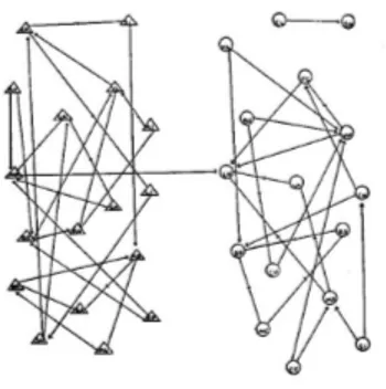
![Figure 1.4: Examples of various types of networks [92]: (a) an undirected network with only a single type of vertex and a single type of edge; (b) a network with a number of discrete vertex and edge types; (c) a network with varying vertex and edge weights](https://thumb-eu.123doks.com/thumbv2/123dokorg/7601689.114409/15.892.328.569.312.522/figure-examples-networks-undirected-network-discrete-network-varying.webp)
![Figure 1.6: The two best studied information networks [92]. Left: the citation network of academic papers in which the vertices are papers and the directed edges are citations of one paper by another](https://thumb-eu.123doks.com/thumbv2/123dokorg/7601689.114409/19.892.243.654.376.640/figure-information-networks-citation-academic-vertices-directed-citations.webp)
![Table 1.2: The macaque and cat cortico-cortical connections [105] are two unweighted networks with respectively N = 69 and N = 55 nodes, K = 413 and K = 564 connections](https://thumb-eu.123doks.com/thumbv2/123dokorg/7601689.114409/51.892.247.654.736.901/macaque-cortico-cortical-connections-unweighted-networks-respectively-connections.webp)