Electrostatic Micro-Electro-Mechanical-Systems
(MEMS) Devices: A Comparison Among Numerical
Techniques for Recovering the Membrane Profile
MARIO VERSACI 1, (Senior Member, IEEE), ALESSANDRA JANNELLI2, AND GIOVANNI ANGIULLI 3, (Senior Member, IEEE)
1Department of Civil, Energy, Environmental and Materials Engineering, Mediterranea University of Reggio Calabria, 89122 Reggio Calabria, Italy 2Department of Mathematics and Information Sciences, Physical Sciences, Earth Science, University of Messina, 98166 Messina, Italy
3Department of Information, Infrastructures and Sustainable Energy Engineering, Mediterranea University of Reggio Calabria, 89122 Reggio Calabria, Italy
Corresponding author: Giovanni Angiulli ([email protected])
ABSTRACT In this work, numerical techniques based on Shooting procedure, Relaxation scheme and Collocation technique have been used for recovering the profile of the membrane of a 1D electrostatic Micro-Electro-Mechanical-Systems (MEMS) device whose analytic model considers |E| proportional to the membrane curvature. The comparison among these numerical techniques has put in evidence the pros and cons of each numerical procedure. Furthermore, useful convergence conditions which ensure the absence of ghost solutions, and a new condition of existence and uniqueness for the solution of the considered differential MEMS model, are obtained and discussed.
INDEX TERMS Electrostatic MEMS devices, non-linear ordinary differential models, shooting method, Keller-Box scheme, Lobatto formulas, ghost solutions.
I. INTRODUCTION
Today there is a growing demand to design high-performance sensors and actuators for cutting-the-edge engineering appli-cations [1]. In such a context, static and dynamic Micro-Electro-Mechanical-Systems (MEMS) technology plays a lead role in implementing these devices [2]. Combining among them micro-size mechanical and electronic devices, MEMS technology, emerged in the second half of the 1960s [3], is now considered as one of the most promising tech-nologies of the 21th century [4], [5]. The industrial usages of MEMS are incredibly varied, ranging from surgical-diagnostic-therapeutic microsystem [6], bio-sensors [7], and tissue engineering [8] to wireless and mobile applications [9]. Furthermore, MEMS are considered extremely interesting for mechatronics applications, because of their small size as well as the easy of realization with relatively low costs [10]. During the years, the advancement in MEMS technology has gone hand in hand with the development of sophisticated theoretical models that more and more adhering to the physics underlying the operation of these devices [2], [5]. Recently, some remarkable results have been achieved in several rele-vant cases, such as thermo-elastic [11], electro-elastic [12], The associate editor coordinating the review of this manuscript and approving it for publication was Mauro Fadda .
and magnetically actuated systems [13]. However, almost all these models are often structured in an implicit form that does not allow to evaluate explicit analytic solutions [14]. Accordingly, these have to be necessarily computed numerically [15]. However, to validate these computational results, analytical conditions ensuring the existence, unique-ness, and regularity of the solutions have to be derived [16]. To this aim, many mathematical models have been theoret-ically conceived by using suitable functional spaces [14]. Along this line, Cassani and coauthors presented in [17] a sophisticated non-linear differential mathematical model of a MEMS device, which, due to its intrinsic complexity, has been subsequently simplified neglecting the inertial and non-local effects [18]. Now, starting from this simplified model, Di Barba et al. have been proposed a new elliptical semi-linear dimensionless model of a 1D membrane MEMS, based on the proportionality between the electric field magnitude |E| and the curvature of the membrane, achieving results of the existence and uniqueness for the solution [19]. In [20] this model was numerically solved by Angiulli et al. by using the Shooting method, whereas in [23] Versaci et al. have developed a new condition of the uniqueness of the solution depending from the material properties and by geometrical characteristics of the device. Based on this premises, in this work we study and compare the numerical performances
of Shooting procedure, Relaxation scheme, and Collocation technique in order to reconstruct the MEMS profile mem-brane. In particular, the Shooting method is an iterative pro-cedure capable of transforming a 1D boundary value problem into an equivalent initial value problem so that the procedure resembles that adopted by a soldier who knows the arrival point of a bullet’s trajectory, but who is in a position to be able to control only the initial values: position of the cannon and speed or height of the shot. he is therefore forced to proceed by attempts, observing the subsequent results in terms of distance from the target and correcting the rise [21], [22]. Concerning the Relaxation procedure, it replace an ordinary differential equation by finite-difference equa-tions on mesh guessing a solution on this mesh. Mathemat-ically, finite-difference equations are just algebraic relations between unknowns. The use of iterative technique to relax this solution allow to get the true solution [21], [22]. Finally, the collocation methods impose the satisfaction of the dif-ferential equation only in selected points of the definition interval. This is equivalent to placing in the internal nodes the differential equation assigned after approximation of the differential operator with an algebraic equivalent, as well as to satisfy the boundary conditions in the edge nodes. The methods summarily described above are notoriously the most effective and efficient for solving numerically boundary value problems. Furthermore, in the literature, regarding the study of electrostatic membrane MEMS, there are no studies comparing the performances obtained with these procedures [21], [22]. Furthermore, we provide new algebraic conditions able to avoid ghost solutions, i.e. numerical solution which do not fit the condition of existence and uniqueness associated to the analytic differential model at hand [20]. As a final result, a new theoretical condition of existence and uniqueness for the solution, which depends from the electromechanical properties of the membrane, is demonstrated. The paper is organized as follows. SectionIIprovides a description of the 1D electrostatic MEMS device considered in this work. The numerical procedures exploited to recover the membrane pro-file are detailed in sectionIII. In sectionIVnumerical results, carried out by using the Matlab R2017a environment running on an Intel Core 2 CPU at 1.45GHZ, are presented. In section Vthe convergence criteria for the considered numerical meth-ods are discussed. Results concerning the existence and the uniqueness of the solution as a function of the electrome-chanical properties of the membrane are demonstrated in sectionVI. In sectionVIIare illustrated the issues regarding the problem of the ghost solutions. Section VIII reports a discussion about the range of parameters for the correct use of the device. Finally, in sectionIXsome conclusive remarks and future perspectives are given.
II. BASICS ON THE 1D ELECTROSTATIC MEMS DEVICE MODEL
A. THE ANALYTIC MODEL
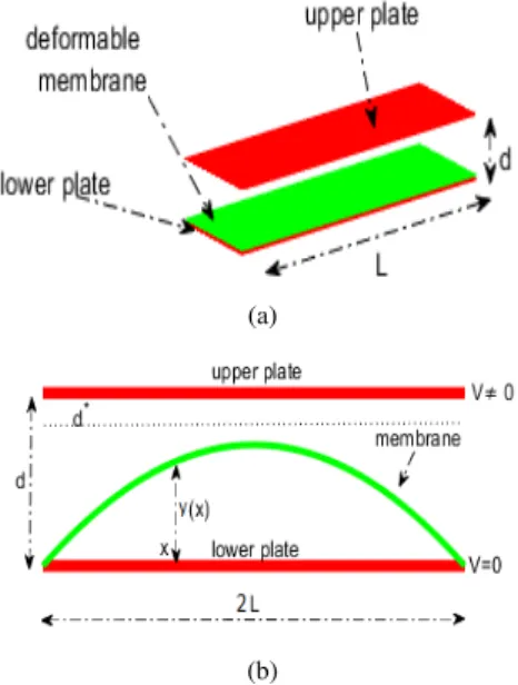
The membrane electrostatic MEMS device considered in this study is shown in Fig. 1a. The upper plate is fixed, whereas
FIGURE 1. (a) Electrostatic MEMS device, (b) Typical profile of a MEMS membrane.
the lower plate has constrained at its edges a membrane. The membrane deforms towards the top plate when an exter-nal voltage V is applied. The corresponding dimensionless model is: 8 < : d2y(x) dx2 = 2 (1 y(x))2, x 2 = [ L, L], y(x) = 0, x 2 @ (1) where y is the profile of the membrane [3], [19]. Since
d ⌧ L, the device can be considered as purely
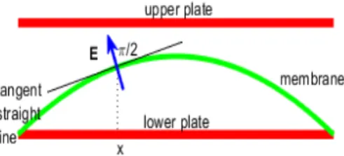
one-dimensional, so that the membrane profile can be described by a continuous function y(x) (see Figure 1b). Taking into account that the electric fieldE is locally orthogonal to the tangent straight line to the membrane, it can be considered proportional to its curvature K (x, y(x)) [24]. Also, because
2
(1 y(x))2 is proportional to |E|2 (that is d 2y(x)
dx2 = ✓|E|2,
✓2 R+), we can derive a more realistic model [19], [20]: 8 > > > > > > > > > < > > > > > > > > > : d2y(x) dx2 = 1 ✓ 2(1 + ( dy(x) dx )2)3(1 d⇤ y(x))2 y = 0 on @ y 2 C2([@]), 0 y(x) < 1 d⇤<1 d2y(x) dx2 2 ( ⇥ R ⇥ R) (2)
in which d⇤is the distance that separates the top of the mem-brane profile from the upper plate (critical security distance). As above mentioned, the device is subjected to an external V , and thus we have that
FIGURE 2. The electrostatic membrane MEMS device:E (blue vector) is
orthogonal to the tangent straight line to the membrane so that |E| can be considered proportional to the curvature of the membrane.
which produces an electrostatic pressure
pel ⇡ 0.5✏0|E|2= 0.5 ✏0V 2
(d y(x))2. (4) This results in a mechanical pressure p = kpel (k constant) that deforms the membrane moving towards the upper plate. Under the condition of maximum deformation, the membrane will be at a critical distance of d⇤from the upper plate.
B. WHEN |E| IS PROPORTIONAL TO K
In [19], the model (1) has been studied observing that 2 / V2, and 2
(1 y(x))2 / |E|2. Accordingly, (1) becomes
8 < : d2y(x) dx2 = ✓|E|2 in = [ L1,L1] y( L1) = y(L1) = 0 ✓ 2 R+, (5) where L1is the half-length of the device. SinceE is locally normal to the tangent straight line of the membrane (see Figure (2)), |E| results proportional to K(x, y(x)), thus we have that [24] K (x, y(x)) = d2y(x) dx2 p (1 + (y(x))2)3, (6)
and |E| can be written as follows:
|E|2 = (µ(x, y(x), ))2(K (x, y(x)))2 = 2(1 y(x)) 2 d2y(x) dx2 2 (1 + (y(x))2) 3 (7) where µ(x, y(x), ) 2 C0([ L 1,L1] ⇥ [0, 1) ⇥ [ min, max]) [19].
III. NUMERICAL APPROACHES
A. SHOOTING PROCEDURE & ODE SOLVERS
To apply the Shooting procedure, we consider a generic second-order non-linear Boundary Value Problem (BVP)
d2y(x)
dx2 = F
⇣
x, y(x),dy(x)dx ⌘: recasting it into a system of first order differential equations [21]:
8 > < > : dy1(x) dx = y2 dy2(x) dx = F(x, y1(x), y2(x)), (8) and by setting 8 < : y1(x) = y(x); y2(x) = dydx1(x)= dy(x)dx , (9) the original BVP (8) is turned into an Initial Value Prob-lem (IVP) by replacing y1(L1) at x = L1with y2( L1) = ⌘, ⌘2 R. Now, integrating this last problem, we achieve y1(L1) at x = L1. If y1(L1) = 0 then we have solved the starting BVP, that in this way defines, implicitly, a non-linear equation of the form
F(⌘) = y1(L1; ⌘) = 0 (10) that can be iteratively solved to find the right value of ⌘ [21]. 1) ZEROS OF F (⌘) = 0: THE DEKKER-BRENT PROCEDURE The Dekker’s approach exploits the bisection procedure to solve a given non linear equation [22]. For each iteration, three points are involved: bk, which approximates temporary the zero; ak, which is the ‘‘contra-point’’ such that F(ak) and
F(bk) have opposite sign, so that the interval [a0,b0] contains the solution, and bk 1, which is the value of b at the previous iteration. Two temporary values are computed: the first one is achieved by the secant procedure, while the second one is obtained by bisection method [21], [22];
8 > < > : s=bk F(bbk bk 1 k) F(bk 1)F(bk) if F(bk) 6= F(bk 1) s = m = ak+ bk2 otherwise. (11) If s (the result of the secant method) is included between bk and m, then s = bk+1, otherwise m = bk+1. The new value of the contra-point is selected so that F(ak+1) and F(bk+1) have different sign. In this case ak+1 = ak., otherwise, ak+1 = bk. Finally, if
|F(ak+1)| < |F(bk+1)|, (12)
ak+1 turns out to be a best approximation of the solution with respect to bk+1, so that ak+1 and bk+1 are exchanged. However, there are circumstances in which each iteration uses the secants method, but the term bk converges very slowly. To avoid this problem, Brent proposed a modification of this strategy inserting a test that must be satisfied before the result of the secant method is accepted for the next iteration. Given a tolerance , if the previous step has been used in the bisection method,
| | < |bk bk 1| (13)
and
| | < |s bk| < 12 |bk bk 1| (14) must be applied to perform the interpolation, otherwise the bisection method is used again. If the previous step used interpolation,
and
| | < |s bk| < 12 |bk 1 bk 2| (16) are applied to decide whether to perform the interpolation (when the inequalities are both satisfied) or the bisection (oth-erwise). This modification ensures that at the kth iteration, the bisection method is used at most for 2 log2⇣|bk 1 bk 2|⌘ times. Furthermore, the Brent method uses inverse quadratic interpolation instead of linear one (as in the secant method). If F(bk), F(ak) and F(bk 1) are different, the efficiency of the method increases slightly. Consequently, the condition to accept s must be changed: s must be between 3ak+bk4 and bk. 2) OBTAINING THE SOLUTION
At each iteration ⌘k is obtained by solving the related IVP. A suitable termination criteria have to be used to verify if ⌘k ! ⌘ as k ! 1. The solutions are obtained by using both teh Matlab built-in functions ode23 and ode45 [22], [25], with the accuracy and adaptivity parameters defined by default. We note that the main difficulty to obtain the solutions concerns the fact that the integration of IVPs that sometimes could be not stable. This means that the solutions of the BVP could be insensitive from the variations of the boundary values, while the solutions of the IVP obtained by the Shooting method are computed through the variations of the initial values [26].
B. RELAXATION PROCEDURE & KELLER-BOX SCHEME In order to apply the relaxation procedure, we employ a mesh of points x0= L1, xj= x0+j1x, for j = 1, 2, . . . , J, evenly spaced with xJ = L1. We denote the numerical approximation to the solution y(xj) of (8) by the 2D vectoryj, j = 0, 1, . . . , J [21], [22]. The Keller Box scheme [27] can be written as follows 8 < : yj yj 1 1F ⇣ xj 1/2yj+ yj 12 ⌘ = 0 j = 1, · · · , J (17)
withG(y0,yJ) = 0 and xj 1/2= (xj+ xj 1)/2. Now, we deal with the system of non-linear equations (17) with respect to the unknown 2(J + 1)-dimensional vector:
y = (y0,y1,· · · , yJ)T. (18) If y(x) and F(x, y) are sufficiently smooth, the solution can be computed by the classical Newton’s method, provided that a sufficiently fine mesh and an accurate initial guess are used. We apply the Newton’s method with the following termination criterion [21] 1 2(J + 1) 2 X `=1 J X j=0 |1yj`| TOL, (19)
where 1yj`, j = 0, 1, . . . , J and ` = 1, 2, is the difference between two successive iterate components and TOL is a fixed tolerance. The adopted initial guess to start the iterations is the following: y1(x) = 1, y2(x) = 1. As far as the accuracy
issue is concerned, the truncation error of the method (17) has an asymptotic expansion in powers of (1x)2[21], [22]. C. COLLOCATION PROCEDURE & III/IV-STAGE LOBATTO IIIa FORMULAS
1) THE COLLOCATION APPROACH
We consider the following system of ordinary differential equations (ODEs) [21]: 8 < : dy(r) dr =F(r, y(r)) G[y(a), y(b)] = 0 (20)
whereG[y(a), y(b)] = 0 represents the boundary conditions. Converting (20) in an integral equation, we obtain:
y(x) = y(xn) + Z x
xn
F(r, y(r))dr. (21)
Replacingy(xn) by the approximated valueyn, we can write: y(x) ⇡ yn+
Z x xn
p(r)dr, (22)
in whichp(r) is an interpolation polynomial of degree lower than s interpoling
[xn,i,F(xn,i),y(xn,i)], i = 1, 2, . . . , s, (23) and
xn,i= xn+ ⌧ih, i = 1, . . . , s,
0 ⌧1< . . . < ⌧s 1. (24) In order to evaluate this polynomial it is possible to exploit the Lagrange or the Newton interpolation polynomial technique [22]. If Lagrange method is exploited, we can write: p(r) = s X j=1 F(xn,j,y(xn,j))Lj(r), (25)
where Lj(r) are the fundamental Lagrange
polynomials [21], [22]. Then, plugging (25) into (22) we obtain: y(x) ⇡ yn+ s X j=1 F(xn,j,y(xn,j)) Z x xn Lj(r)dr. (26) Then, (26) is forced for all the xn,j, so thatyn,jat collocation node points are obtained, for i = 1, . . . , s, by:
yn,j= yn+ s X j=1 F(xxn,i,ynn,j) Z xn,i xn Lj(r)dr. (27) If ⌧s= 1, yn+1= yn,s, (28) otherwise: yn+1= yn+ s X j=1 F(xn,j,yn,j) Z xn+1 xn Lj(r)dr. (29) Collocation methods are reliable tools, although may not be suitable if high accuracy is required [21].
2) IMPLICIT RUNGE-KUTTA PROCEDURES
Runge-Kutta (RK) methods involve many evaluations of the function F(x, y(x)) in each interval [xn,xn+1]. In its more general form, an RK method can be written in the following way [22]: yn+1 = yn+ h s X i=1 biki (30) where ki= F ⇣ xn+ cih, yn+ h s X j=1 aijkj ⌘ , i = 1, 2, . . . , s (31) where s denotes the number of stage of the procedure. Coefficients{aij}, {ci} and {bi} characterize a RK procedure and can be collected in the Butcher Tableau [21], [22]
c A
bT (32)
where A = (aij) 2 Rs⇥s, b = (b1, . . . ,bs)T 2 Rs and c = (c1, . . . ,cs)T 2 Rs. IF coefficients aijare equal to zero for j i, with i = 1, 2, . . . , s, then each ki can be explic-itly computed exploiting the i 1 coefficients k1. . .ki 1 which have already been calculated. Then, RK procedure is called explicit. Otherwise, it is said implicit. and to compute the coefficient ki one has solve a s-dimensional non-linear system. To construct an implicit RK methods one needs to consider three conditions as follows [21]:
B(p) : s X i=1 bick 1i = k 1, k = 1, 2, . . . , p (33) C(q) : s X i=1 aijck 1i = k 1cki, k = 1, 2, . . . , p, i = 1, 2, . . . , s (34) D(r) : s X i=1 bick 1i aij= k 1bj(1 ckj), k = 1, 2, . . . , r, j = 1, 2, . . . , s. (35) Condition (33) means that the following quadrature formula
Z x+h x F(s)ds ⇡ h s X i=1 biF(x + cih) (36)
is exact for all polynomials whose degree is lower than p. If (33) is satisfied, then the RK method has quadrature of order q. Analogously for condition (34). In other words, if it is satisfied, then the corresponding quadratures
Z t+cih x F(s)ds ⇡ h s X j=1 aijF(x + cjh) (37)
are exact for all polynomials whose degree are lower than q. In this case the RK procedure is of stage of order q. It is proved that all methods satisfying condition (34) having ci,
i = 1, 2, . . . , s distinct are collocation procedures.
In order to simplify the construction of an implicit Runge-Kutta procedure, one can exploit the following well-known Lemma [21], [22].
Lemma 1: Let us consider a RK procedure with s stage
having c1 6= c2 6= . . . 6= cs. In addition, let be bj,
j = 1, 2, . . . , s. Then, the two following statements occurs:
1. C(s) ^ B(s + ⌫) ) D(⌫) 2. D(s) ^ B(s + ⌫) ) C(⌫)
so that one ca built the procedure exploiting B(p) and
D(r) or C(q).
3) THE THREE-STAGE LOBATTO IIIa FORMULA
This procedure requires that the coefficient cimust be chosen as roots of [21]:
P⇤s P⇤ s 2=
ds 2
dxs 2(xs 1(x 1)s 1), (38) where s is the number of the stage, obtaining in this way
c1= 0 and cs= 1 8s, so that the quadrature formula is exact for any polynomial whose degree is less than 2s 2 [28].
Let us premise the following two definitions.
Definition 1 (Definition of the Step-Size): Let us consider
the following mesh-grid:
0 = a = r0<r1< . . . <rn= b = R (39) and, on it, let us define the step -size hm= rm+1 rm.
Definition 2 (Midpoint and Approximation at the Mid-point): Starting from (rm,rm 1), we denote their midpoints by rm+1/2and by ym+1/2the approximation of y(r) at rm+1/2.
Remark 1 (On the Order of the Polynomial): The cubic polynomialp(r) satisfy the boundary conditions in (20) and, in addition, 8(rm,rm+1), the subdivision (39) is taken into account. In addition,p(r) is located at the edges of each sub-interval and midpoint as well wherep(r) is continuous.
This approach is a collocation procedure and it is proved that is totally equivalent to the three-stage Lobatto IIIa implicit RK procedure [28] whose Butcher tableau is [21]
0 0 0 0 1 2 5 24 1 3 1 24 1 1 6 2 3 1 6 1 6 2 3 1 6 (40)
Then, the three-stage Lobatto IIIa formula can be written as follows [21]: ym+1/2 = ym+ hm 524F(rm,ym) +13F(rm+1/2,ym+1/2) 1 24F(rm+1,ym+1) (41) ym+1 = ym+ hm 16F(rm,ym) +23F(rm+1/2,ym+1/2) +1 6F(rm+1,ym+1) . (42)
Remark 2 (On the Use of Simpson Quadrature Formula):
This procedure can be derived from the (21) exploiting the Simpson quadrature formula to approximate the integral between xnand x. Obviously, when the procedure is applied to a quadrature problem, it reduces (42) to the well-known Simpson formula [22]: ym+1 = ym+h6m F(rm,ym) (43) + F(rm+1,ym+1) + 4F ⇢ rm+1/2,ym+1+ ym 2 +h8m[F(rm,F(rm,ym) F(rm+1,ym+1)] . (44)
Remark 3 (On the Polynomial p(r) and Its Derivatives:
Collocation Polynomial): We note that p(r) and their derivaties satisfy, 8r 2 (a, b) [28],
p(l)(r) = y(l)(r) + O(h4 l), l = 0, 1, 2, 3. (45) Furthermore, equations (20) are satisfied by p(r) at each intermediate point and at the midpoint of each interval as well (collocation polynomial). It is worth nothing that the form of p(r) is chosen by Matlab by means of the determination of unknown parameters, if any. Finally, we can write:
8 > < > : p0(rm) = F[rm,p(rm)] p0(rm+1/2) = F[rm+1/2,p(rm+1/2)], p0(rm+1) = F[rm+1,p(rm+1)] (46) which represent non-linear equations that can be solved by a Matlab solver. Moreover, Matlab, 8r 2 (a, b), evalu-ates the cubic polynomial by means of its special function
bvpval [25].
Remark 4 (A Guess for the Solution & Initial Mesh): It is
known that a BVP could have more than one solution [22]. Then, it is important to supply a guess for both the initial mess and the solution as well. Obviously, the Matlab solver adapt the mesh obtaining a solution by means of a reduced number of mesh points [25].
It is worth noting that, very often, a good initial hypothesis is extremely complicated. Then, the Matlab solver acts by checking a residue defined as [25]:
res(r) = p0(r) F[r, p(r)]. (47)
while the boundary conditions becomeg[p(a), p(b)]. Obvi-ously, ifres(r) is small, then p(r) represents a good solution and, in the case of well-conditioned problem,p(r) is close to y(r). In this paper, the the Matlab R2017a bvp4c solver has been exploited because, firstly, it implements the collocation technique by means of a piecewise cubicp(r), whose coef-ficients are determined requiring thatp(r) be continuous on (a, b). Moreover, both mesh and estimation error are based on the evaluation of the residual of p(r) whose control is useful to manage poor or inadequate guesses for both mesh and solution [25]. In addition, this Toolbox presents a very
reduced computational complexity to achieve the Jacobian
J = @@Fy =i 2 6 6 4 @F1 @y1 @F1 @y2 @F2 @y1 @F2 @y2. 3 7 7 5 (48)
Finally, being bvp4c a vectorized solver, it is able to strongly reduce the run-time vectorizingF(r, y(r)) [25].
4) FOUR-STAGE LOBATTO IIIa FORMULA
This formula is derived as an implicit RK procedure whose Butcher tableau is the following [21]:
0 0 0 0 0 5 p5 10 11 +p5 120 25 p5 120 25 13p5 120 1 +p5 120 5 +p5 10 11 p5 120 25 + 13p5 120 25 +p5 120 1 p5 120 1 1 12 5 12 5 12 1 12 1 12 5 12 5 12 1 12 (49) As the three-stage formula, this approach is a polynomial collocation procedure providing solutions belonging to the space C1([a, b]) with accuracy of the fifth-order. Unlike the bvp4c solver that exploits analytical condensation procedure,
Matlab solves the four-stage Lobatto IIIA formula by finite difference approach (bvp5c solver) and solves the algebraic equations directly. Moreover, unlike bvp4c solver that han-dles the unknown parameters directly, bvp5c solver augments the system with trivial differential equations for unknown parameters [21], [22], [25].
IV. NUMERICAL RESULTS
In this section, we present the numerical results obtained by using the numerical procedures discussed in the previous section. At this purpose, we rewrite (2) as a system of first order ODEs, and applying (8) and (9), we can write:
8 > > > > < > > > > : dy1(x) dx = y2(x) dy2(x) dx = 1 ✓ 2(1 + y 2 2(x))3(↵ y1(x))2, y1( L1) = y1(L1) = 0 (50)
Remark 5: It is worth nothing that if y(x) = 1 d⇤, from the model (2) it can be seen that d2dxy(x)2 = 0. In other words,
this condition has no physical relevance because from the model (1) (or model (5)) we would supply |E| = 0 with linear deflection of the membrane.
Figure 3 shows the numerical results for the membrane profile y(x) computed by using different values of the param-eter ✓ 2exploiting the Shooting method implemented by the
FIGURE 3. Profile of the membrane y(x) for different values of ✓ 2when the shooting procedure & ode23 ToolBox Matlab is exploited. The deflection of the membrane increases when ✓ 2decreases.
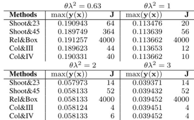
Matlab built-in function ode23. It can be noted that the mini-mum value of this parameter that guarantees the convergence of the procedures is equal to ✓ 2 = 0.63. Similar results are obtained by applying the other numerical approaches. For all computation, we choose d⇤ = 10 4and L1 = 0.5. For the Shooting method & ODE solvers (Shoot&23 and Shoot&45), we set y1(0) = 1 and y2(0) = 1.2 as initial guess for ✓ 2 = 0, 63, 1, 4 and y1(0) = 0.1 and y2(0) = 0.2 as initial guess for ✓ 2 = 2, 3. For the relaxation procedure & Keller box scheme (Rel&Box), we set both initial guesses as
y1(0) = y2(0) = 1. Finally, y1(0) = y2(0) = 0 are set for the collocation procedure & Lobatto formulae (Col&III and Col&IV). A comparison of the results obtained for values of ✓ 2= 0.63, 1, 2, 3 is reported in Table1. Finally, with ✓ 2= 4, we obtain the same value max(y(x)) = 0.029918, for a number of grid points equal to J = 14, 52, 4000, 4, 6, respec-tively. The numerical results demonstrate that each numerical procedure considered in this study shows an excellent perfor-mance in recovering the membrane profile. However, it can be noticed as the profile is computed exploiting for each method a different order of accuracy and a different number of grid points. We have that both the relaxation method and the Keller box scheme reveals robust and accurate. Notably, the Keller box provides results as accurate as those of the Shooting and collocation method, because it involves more grid points are for its computations. However, because of that, it is slower and has a higher computational cost than these methods. The Shooting method is not as robust as the relaxation and the collocation methods, but it has the advantage of the speed and adaptivity of the Matlab built-in functions ode23 and
ode45, that have been used for solving the related IVPs.
Finally, the collocation method provides a solution by using very few numbers of grid points. This because the profile is not characterized by hardly sharp changes. Now, although all the considered numerical approaches represent efficient and reliable tools for solving the BVPs in the case of convergence conditions ensuring the absence of ghost solutions, we can
TABLE 1.Comparison of the results for different values of the parameter ✓ 2.
conclude that the relaxation approach and the Keller box scheme reveals more robust in all performed numerical tests. V. CONVERGENCE OF THE NUMERICAL APPROACHES Indicating by [(✓ 2)
conv]Sode23the range of ✓ 2ensuring con-vergence by means of shooting procedure exploiting ode23 MatlabR, in [23] it was experimentally achieved that
[(✓ 2)conv]Sode23 = [0.63, +1) (51) so that if
[(✓ 2)no conv]Sode23 = [0, 0.63) (52) the convergence of the numerical procedure is not ensured. In addition, exploiting the Keller-Box scheme, in [26], the experimental range of ✓ 2ensuring convergence was
[(✓ 2)conv]Keller Box = [0.592, +1). (53) Also in this case, if
[(✓ 2)no conv]Keller Box = [0, 0.592) (54) the convergence of the Keller-Box scheme procedure is not ensured. In this paper, the experimental range of ✓ 2ensuring convergence when the Shooting procedure exploiting ode45 MatlabR is applied, has been achieved. In particular, as for Shooting with ode23 MatLabR
[(✓ 2)conv]Sode45 = [0.63, +1) (55) and the range that does not ensure convergence, for this case, is:
[(✓ 2)no conv]Sode45 = [0, 0.63). (56) Finally, applying both Three and Four Stage Lobatto IIIa Formulas we have experimentally achieved
[(✓ 2)conv]ThreeStageLobatto = [1.181, +1) (57) and
[(✓ 2)conv]FourStageLobatto = [1.181, +1) (58) so that, for both Three and Four Stage Lobatto IIIa Formulas, the range of ✓ 2that does not ensure the convergence is:
TABLE 2. For each exploited numerical procedure, the ranges of ✓ 2 ensuring convergence.
Table 2 summarizes these conditions. In the event that all numerical procedures worked in parallel, we are interested in knowing the minimum value of ✓ 2above which the con-vergence of at least one numerical procedure is guaranteed. Then, the following makes sense:
min(✓ 2)conv
= minnmin[(✓ 2)conv]Sode23, min[(✓ 2)conv]Keller Box, min[(✓ 2)conv]Sode45,
min[(✓ 2)conv]ThreeStageLobatto, min[(✓ 2)
conv]FourStageLobatto o
= 0.592. (60)
In other words, for values greater than or equal to 0.592 the convergence of at least one numerical solution is guaranteed. Accordingly, for ✓ 2 0.63 the convergence is guaranteed for all the methods. However, we point out that even if a numerical solution is obtained, we must be sure that this satisfy the analytical condition of existence and uniqueness for (2) if we want to avoid the possibility of evaluating a potential ghost solution.
VI. EXISTENCE AND UNIQUENESS OF THE SOLUTION DEPENDING ON THE ELECTROMECHANICAL PROPERTIES OF THE MEMBRANE
In [19] the problem of the existence and uniqueness of the solution for (2) has been studied demonstrating that: i) the uniqueness is always guaranteed, and that ii) the existence conditions take the form:
1 +⇣supn dy(x) dx o⌘6 <0.5(↵L1) 1 ⇣ supn dy(x) dx o⌘ ✓ 2 (61)
where the parameter 2depends by the minimum value of the applied voltage V needed to overcome the membrane inertia. Moreover, in [19], it was demonstrated that:
supn dy(x)
dx
o
= 99. (62)
Remark 6: It is worth noting that sup{|dy(x)dx |} = 99 is quite high. This is due to the fact that a large number of increases
were necessary to obtain the condition (61). In any case, the value obtained, albeit high, is certainly a safety advantage.
Remark 7: It is also observable that, in [19], the
unique-ness of the solution for the (2) problem is always guaranteed. However, the proof, using the joint use of Poincaré inequality and the Gronwall Lemma, did not highlight behaviors depen-dent on the electromechanical characteristics of the material constituting the membrane. In other words, uniqueness was always guaranteed regardless of the material constituting the membrane.
In what follows, we present a new condition that links the uniqueness of the solution for (2) to the electromechanical properties of the MEMS membrane:
Theorem 1: Let us consider problem (2). If 1 +⇣supn dy(x)
dx
o⌘6
<(24L1(L1+ 1)) 1✓ 2 (63) then (2) admits unique solution.
Proof: see appendix.
Finally, in order to achieve a unique condition that ensures both existence and uniqueness, we have to solve the following system: 8 > > > > > > > < > > > > > > > : 1 +⇣supn dy(x) dx o⌘6 <0.5(↵L1) 1✓ 2 ⇣ supn dy(x) dx o⌘ 1 +⇣supn dy(x) dx o⌘6 <(6L1(L1+ 1)) 1✓ 2. (64)
The system (64) is equivalent to (63). This last relation is of paramount importance because it reduces the risk to compute ghost solutions.
VII. CONVERGENCE AND GHOST SOLUTIONS
Taking into account that L1 = 0.5, from (63) and (62), we obtain that ✓ 2 18 so that if ✓ 2 2 [18, +1) we have that both existence and uniqueness for (2) are ensured. Moreover, it is known that [19]:
2= ✏0L12V2 d3T <
✏0L12V2
(1 d⇤)3T. (65)
Multiplying the above relation for ✓, we obtain: ✓ 2< ✓ ✏0L
2 1V2
(1 d⇤)3T. (66)
Combining (63) and (66), we can write: 1 +⇣supn dy(x) dx o⌘6 < ✓ 2 24L1(1 + L1) ✓ ✏0L 2 1V2 24L1(1 + L1)(1 d⇤)3T, (67) from which: 24L1(1 + L1) ⇣⇣ supn dy(x) dx o⌘6 ) < ✓ 2 ✓ ✏0L 2 1 (1 d⇤)3T. (68)
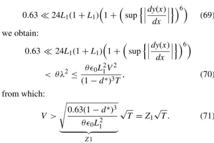
But noting that: 0.63 ⌧ 24L1(1 + L1) ⇣ 1 +⇣supn dy(x) dx o⌘6⌘ (69) we obtain: 0.63 ⌧ 24L1(1 + L1) ⇣ 1 +⇣supn dy(x) dx o⌘6⌘ < ✓ 2 ✓ ✏0L 2 1V2 (1 d⇤)3T, (70) from which: V > s 0.63(1 d⇤)3 ✓ ✏0L12 | {z } Z1 p T = Z1pT . (71) This last relation highlights that thicker the membrane, the higher the voltage V to be applied to the device for overcoming the inertia of the membrane itself. In addition, since: 18 ⌧ 24L1(1 + L1) ⇣ 1 +⇣supn dy(x) dx o⌘6⌘ , (72) we can write: V > s 18(1 d⇤)3 ✓ ✏0L12 | {z } Z2 p T = Z2pT , (73) so that both (71) and (73) identify, the plane formed by the mechanical tension T and the applied external voltage V, areas of convergence in the presence/absence of ghost solu-tions. As shown in Figure4, (71) defines the non-convergence area for each numerical procedure (area below the blue curve). On the other hand, between the blue and red curves, the convergence is of at least one numerical procedure is high-lighted, but the absence of ghost solutions is not guaranteed. Finally, above the red curve, the area where both convergence and absence of ghost solution are guaranteed is highlighted.
FIGURE 4. T V plane partitioned into three distinct areas: non-convergence area; convergence with ghost solutions area; convergence without ghost solutions area.
Remark 8: We note that ensuring the absence of ghost
solutions is very important for MEMS devices. This is because it allows, on the one hand, to recover membrane profiles compatible with the geometry of the device and, on the other, to obtain ranges of possible values for V , |E| and
T able to define with sufficient rigor operating conditions to
which the device must be subjected.
VIII. RANGE OF PARAMETERS FOR THE CORRECT USE OF THE DEVICE
As previously described, MEMS devices subjected to exter-nal V force the membrane to deform towards the upper plate. Therefore, it seems natural to ask, once the material constituting the membrane (ie, fixed T ) has been chosen, what the range of possible values must be for V and |E| able to obtain membrane profiles compatible with the device geometry. Vice versa, having fixed the intended use of the device (i.e. fixed V and |E|), we also ask which material is most suitable for building the membrane. With this aim in mind, starting from (63) and (66), and considering that
L1= 0.5, we can easily write: 1+⇣supn dy(x) dx o⌘6 < ✓ 2 18 =18✓ ✏0dL312TV2< ✓ 18 ✏0L12V2 (1 d⇤)3T, (74) from which: ⇣ supn dy(x) dx o⌘ < 6 s ✓ 18 ✏0L12V2 (1 d⇤)3T 1, (75)
that provides the range of admissible values of supn dy(x)dx o, once known i) the electromechanical properties of the mem-brane (✓), ii) the lower plate mechanical tension T for V = 0, and iii) the applied voltage V . Moreover, we can write:
✓|E|2= 2 (1 y(x))2 = 1 (1 y(x))2 ✏0L12V2 d3T < 1 (1 y(x))2 ✏0L12V2 (1 d⇤)3T. (76)
In addition being 1 y(x) > 1 d⇤, we have that 1 (1 y(x))2 <
1
(1 d⇤)2 from which the condition (76) becomes:
✓|E|2< ✏0L 2 1V2 (1 d⇤)5T, (77) finally obtaining |E| V = s ✏0L12 (1 d⇤)5T ✓. (78)
By (78), fixing the electromechanical properties of the mem-brane ✓ and the mechanical tension T , we obtain the ratio between |E| and V , which are the operative electrostatic
parameters of the device. Vice versa, starting from (77), we can also write:
T ✓ < ✏0L12V2
(1 d⇤)5|E|2, (79)
so that, starting from the knowledge of the couple (|E|, V ), we obtain T ✓.
IX. CONCLUSION
In order to recover the membrane profile of a 1D model of an electrostatic membrane MEMS device, in which |E| is locally proportional to the membrane curvature, in this work the Shooting procedure, the Relaxation scheme, and the Colloca-tion technique, have been exploited. Numerical results have highlighted a better performance of the Relaxation & Keller-Box method compared to Shooting procedure and the Lobatto formulas. However, although the relaxation procedure offers the best performance, it requires a higher computational time (a large number of grid points) than the other approaches. Also, we have determined in the plane formed by the mechan-ical tension T and the applied external voltage V, the areas where the numerical procedures can converge with or without these being affected by possible ghost solutions. Finally, a new condition of existence and uniqueness, which depends on the device geometry and the electromechanical properties of the membrane, has been obtained. To conclude, we point out that, despite the differential model considered in this work results being simplified in some aspects, the obtained numeri-cal results provide sufficient qualitative pieces of information to analyze MEMS device characterized by simple geometry. Anyway, to improve its adherence to the experimental ones, it appears of paramount importance to improve the MEMS differential model considered in the present study, taking into account more sophisticated geometrical curvature formula-tions.
APPENDIX
PROOF OF THEOREM 1
Let us consider two different solutions y1(x), y2(x) 2 P, where: P =nC02() : 0 < y(x) < ↵, dy(x) dx <sup n dy(x) dx o <+1 o . (80) The proof of the Theorem is divided into three steps:
Step 1. We prove that ⇣ 1 +⇣ dydx2(x)⌘2⌘3 ⇣1 +⇣ dydx1(x)⌘2⌘3 24⇣supn dy(x) dx o⌘5 dy2(x) dx dy1(x) dx . (81)
In fact, considering that supn dy(x)dx o>1, we can write: ⇣ 1 +⇣ dydx2(x)⌘2⌘3 ⇣1 +⇣ dydx1(x)⌘2⌘3 = h⇣ dydx2(x)⌘2 ⇣ dydx1(x)⌘2i ⇥h⇣1 +⇣ dydx1(x)⌘2⌘2+⇣1 +⇣ dydx2(x)⌘2⌘ ⇥⇣1 +⇣ dydx1(x)⌘2⌘+⇣1 +⇣ dydx2(x)⌘2⌘2i 2⇣supn dy(x) dx o⌘ dy2(x) dx dy1(x) dx ⇥h⇣1 +⇣supn dy(x) dx o⌘2⌘2 +⇣1 +⇣supn dy(x) dx o⌘2⌘ ⇥⇣1 +⇣supn dy(x) dx o⌘2⌘ +⇣1 +⇣supn dy(x) dx o⌘2⌘2i = 2⇣supn dy(x) dx o⌘ dy2(x) dx dy1(x) dx ⇥⇣1 +⇣supn dy(x) dx o⌘2⌘2 +⇣1 +⇣supn dy(x) dx o⌘2⌘2 +⇣1 +⇣supn dy(x) dx o⌘2⌘2 = dydx2(x) dydx1(x) ⇣6⇣supn dy(x) dx o⌘ +6⇣supn dy(x) dx o⌘5 + 12⇣supn dy(x) dx o⌘3⌘ 24⇣supn dy(x) dx o⌘5 dy2(x) dx dy1(x) dx . (82)
Step 2. We prove that: ⇣ 1 +⇣ dydx2(x)⌘2⌘3(↵ y2(x))2 ⇣ 1 +⇣ dydx1(x)⌘2⌘3(↵ y1(x))2 216⇣supn dy(x) dx o⌘5 dy2(x) dx dy1(x) dx + 24(1 +⇣supn dy(x) dx o⌘6 ) y2(x) y1(x) . (83) In fact, 8 y1(x), y2(x) 2 P, since ↵ < 1 because 0 < u < 1 d⇤, it follows that: ⇣ 1 +⇣ dydx2(x)⌘2⌘3(1 d⇤ y2(x))2 ⇣ 1 +⇣ dydx1(x)⌘2⌘3(1 d⇤ y1(x))2 = ⇣1 +⇣ dydx2(x)⌘2⌘3⇣1 + d⇤+ y22(x) 2d⇤ 2y2(x) + 2y2(x)d⇤ ⌘ ⇣ 1 +⇣ dydx1(x)⌘2⌘3 ⇥⇣1 + d⇤+ y2 1(x) 2d⇤ 2y1(x) + 2y1(x)d⇤ ⌘ = ⇣1 +⇣ y2dx(x)⌘2⌘3+ d⇤⇣1 +⇣ dy2(x) dx ⌘2⌘3 + y22(x) ⇣ 1 +⇣ dydx2(x)⌘2⌘3
2d⇤⇣1 +⇣ y2(x) dx ⌘2⌘3 2y2(x) ⇣ 1 +⇣ dydx2(x)⌘2⌘3 + 2y2(x)d⇤ ⇣ 1 +⇣ dydx2(x)⌘2⌘3 ⇣ 1 +⇣ dydx1(x)⌘2⌘3 d⇤⇣1 +⇣ dy1(x) dx ⌘2⌘3 y21(x)⇣1 +⇣ dy1(x) dx ⌘2⌘3 + 2d⇤⇣1 +⇣ dydx1(x)⌘2⌘3 + 2y1(x) ⇣ 1 +⇣ dydx1(x)⌘2⌘3 2y1(x)d⇤ ⇣ 1 +⇣ dydx1(x)⌘2⌘3 (1 +⇣ dydx2(x)⌘2⌘3 ⇣1 +⇣ dydx1(x)⌘2⌘3 + y22(x) ⇣ 1 +⇣ dydx2(x)⌘2⌘3 y22(x)⇣1 +⇣ dy1(x) dx ⌘2⌘3 + y22(x) ⇣ 1 +⇣ dydx1(x)⌘2⌘3 y21(x)⇣1 +⇣ dy1(x) dx ⌘2⌘3 + d⇤⇣1 +⇣ dydx2(x)⌘2⌘3 ⇣1 +⇣ dydx1(x)⌘2⌘3 + 2d⇤ ⇣1 +⇣ dydx2(x)⌘2⌘3 ⇣1 +⇣ dydx1(x)⌘2⌘3 + 2 y2 ⇣ 1 +⇣ dydx2(x)⌘2⌘3 y2(x) ⇣ 1 +⇣ dydx1(x)⌘2⌘3 + y2(x) ⇣ 1 +⇣ y1dx(x)⌘2⌘3 y1(x) ⇣ 1 +⇣ dydx1(x)⌘2⌘3 + 2d⇤ y2(x) ⇣ 1 +⇣ dydx2(x)⌘2⌘3 y2(x) ⇣ 1 +⇣ dydx1(x)⌘2⌘3 + y2(x) ⇣ 1 +⇣ dydx1(x)⌘2⌘3 y1(x) ⇣ 1 +⇣ dydx1(x)⌘2⌘3 216⇣supn dy(x) dx o⌘5 dy2(x) dx dy1(x) dx + 24⇣1 +⇣supn dy(x) dx o⌘6⌘ y2(x) y1(x) . (84)
Step 3. This point is demonstrated by contradiction. We assume that y1(x), y2(x) 2 P are two different solutions. By differentiation and exploiting a suitable Green’s func-tion 6(x, s), (2) can be written into an equivalent integral
formulation. Then, for i = 1, 2, we can write:
yi(x) = Z L1 L1 6(x, s) ⇣ 1 +⇣dydsi(s) ⌘2⌘3 ✓ µ2(s, yi(s), ) ds = Z L1 L1 1 ✓ 26(x, s) ⇥⇣1 +⇣ dyids(s)⌘2⌘3(↵ yi(s))2ds (85) dyi(x) dx = Z L1 L1 d6(x, s) dx ⇣ 1 +⇣dy1(s) ds ⌘2⌘3 ✓ µ2(s, yi(s), ) ds = Z L1 L1 1 ✓ 2 d6(x, s) ds ⇥⇣1 +⇣ dyi(s)ds ⌘2⌘3(↵ yi(s))2ds. (86) Then, it follows that:
||y1(x) y2(x)||C1([ L1,L1]) = sup x2[ L1,L1] |y1(x) y2(x)| + sup x2[ L1,L1] dy1(x) dx dy2(x) dx . (87)
Then, it follows that: ||T (y1) T (y2)|| = 1 ✓ 2x2[ Lsup1,L1] Z L1 L1 6(x, s)((1 + (y01(s))2)3) ⇥(↵ y1(s))2ds Z L1 L1 6(x, s) ⇥((1 + (y02(s))2)3)(↵ y2(s))2ds + 1 ✓ 2x2[ Lsup1,L1] Z L1 L1 d6(x, s) dx ⇥((1 + (y01(s))2)3)(↵ y1(s))2ds Z L1 L1 d6(x, s) dx ((1 + (y02(s)) 2)3) ⇥(↵ y2(s))2ds 1 ✓ 2 L1 2 ⇥ sup x2[ L1,L1] Z L1 L1 [( (1 + (y0 1(s))2)3)(↵ y1(s))2 + (1 + (y02(s))2)3)(↵ y2(s))2]ds +2✓12 sup x2[ L1,L1] Z L1 L1 [( (1 + (y01(s))2)3) ⇥(↵ y1(s))2 + (1 + (y02(s))2)3)(↵ y2(s))]ds = 1 ✓ 2 ⇣ 0.5 + 0.5L1 ⌘
⇥ sup x2[ L1,L1] Z L1 L1 [( (1 + (y01(s))2)3) ⇥(↵ y1(s))2+ (1 + (y02(s))2)3)(↵ y2(s))]ds . (88) Considering (84), we can write:
||T (y1) T (y2)||C1([ L1,L1]) 1 ✓ 2(0.5 + 0.5L1) ⇥ sup x2[ L1,L1] Z L1 L1 ⇣ 216⇣supn dy(x) dx o⌘5 ⇥ dyds2(s) dyds1(s) + 24⇣1 +⇣supn dy(x) dx o⌘6⌘ ⇥|y2 y1|)ds = 1 ✓ 2 ⇣ 0.5 + 0.5L1 ⌘ ⇥⇣216⇣supn dy(x) dx o⌘5 2L1 ⌘ ⇥ sup s2[ L1,L1] dv2(s) ds dv1(s) ds + 1 ✓ 2 ⇣ 0.5 + 0.5L1 ⌘ ⇥⇣24⇣1 +⇣supn dy(x) dx o⌘6⌘ 2L1 ⌘ ⇥ sup s2[ L1,L1] |y2(s) y1(s)|. (89)
We observe that, y1= T (y1) and y2= T (y2) so that, exploit-ing both (87) and (89), we would obtain a contradiction if we write: 8 > > > > > > > > > < > > > > > > > > > : 216 · 2L1(✓ 2) 1 ⇣ 0.5 + 0.5L1 ⌘ ·⇣supn dy(x) dx o⌘5 <1; 24 · 2L1(✓ 2) 1 ⇣ 0.5 + 0.5L1 ⌘ ·⇣1 +⇣supn dy(x) dx o⌘6⌘ <1, (90) that is: 8 > > > > < > > > > : 216⇣supn dy(x) dx o⌘5 <(L1(L1+ 1)) 1✓ 2 24⇣1 +⇣supn dy(x) dx o⌘6⌘ <(L1(L1+ 1)) 1✓ 2. (91)
From the first inequality of (91), it makes sense to write: 1 +⇣supn dy(x) dx o⌘6 <1 + (216L1(L1+ 1)) 1✓ 2 ⇣ supn dy(x) dx o⌘ , (92)
so (91) assumes the following form: 8 > > > > > > > < > > > > > > > : 1 +⇣supn dy(x) dx o⌘6 <1 + (216L1(L1+ 1)) 1✓ 2 ⇣ supn dy(x) dx o⌘ 1 +⇣supn dy(x) dx o⌘6 <(216L1(L1+ 1)) 1✓ 2. (93)
Furthermore, we observe that: (24L1(L1+ 1)) 1✓ 2 <1 + (216L1(L1+ 1)) 1✓ ⇣ supn dy(x) dx o⌘ , (94)
in fact, starting from (94), it follows that: ⇣
supn dy(x)
dx
o⌘
>9(1 24(✓ 2) 1L1(L1+ 1)). (95) That is definitely true. In fact, supposing, by contradiction, that 24L1(L1+ 1) 1✓ 2 >1 + (216L1(L1+ 1)) 1✓ 2 ⇣ supn dy(x) dx o⌘ , (96) we can write: ⇣ supn dy(x) dx o⌘ <9 216(✓ 2) 1L1(L1+ 1) < 0. (97) In other words, ⇣supn dy(x)dx o⌘ assumes a negative value (value physically impossible). Then, (63) holds so that the uniqueness of the solution depends on the physical param-eters of the membrane. Moreover, 2does not appear, con-firming the experimental fact that when V is applied, the membrane moves if V overcomes the inertia 2.
REFERENCES
[1] S. Saponara and A. De Gloria, Eds., Applications in Electronics Pervading Industry, Environment and Society: APPLEPIES 2018 (Lecture Notes in Electrical Engineering Book), vol. 573. Springer, 2019.
[2] J. Zhu, X. Liu, Q. Shi, T. He, Z. Sun, X. Guo, W. Liu, O. B. Sulaiman, B. Dong, and C. Lee, ‘‘Development trends and perspectives of future sen-sors and MEMS/NEMS,’’ Micromachines, vol. 11, no. 1, p. 7, Dec. 2019. [3] J. A. Pelesko and D. H. Bernstein, Modeling MEMS and NEMS.
Boca Raton, FL, USA: CRC Press, 2003.
[4] D. Ortloff, T. Schmidt, K. Hahn, T. Bieniek, G. Janczyk, and R. Brück, MEMS Product Engineering. Vienna, Austria: Springer-Verlag, 2014. [5] M. Gad-El-Hak, The MEMS Handbook. Boca Raton, FL, USA: CRC Press,
2015.
[6] F. Khoshnoud and C. W. de Silva, ‘‘Recent advances in MEMS sen-sor technology—Biomedical applications,’’ IEEE Instrum. Meas. Mag., vol. 15, no. 1, pp. 8–14, Feb. 2012.
[7] C. Walk, M. Wiemann, M. Görtz, J. Weidenmüller, A. Jupe, and K. Seidl, ‘‘A piezoelectric flexural plate wave (FPW) bio-MEMS sensor with improved molecular mass detection for point-of-care diagnostics,’’ Current Directions Biomed. Eng., vol. 5, no. 1, pp. 265–268, Sep. 2019. [8] C. M. Puleo, H.-C. Yeh, and T.-H. Wang, ‘‘Applications of MEMS
technologies in tissue engineering,’’ Tissue Eng., vol. 13, no. 12, pp. 2839–2854, Dec. 2007.
[9] P. A. Kumar, K. S. Rao, and K. G. Sravani, ‘‘Design and simulation of mil-limeter wave reconfigurable antenna using iterative meandered RF MEMS switch for 5G mobile communications,’’ Microsyst. Technol., vol. 26, pp. 2267–2277, Sep. 2019.
[10] A. A. Zhilenkov and D. Denk, ‘‘Based on MEMS sensors man-machine interface for mechatronic objects control,’’ in Proc. IEEE Conf. Rus-sian Young Researchers Electr. Electron. Eng. (EIConRus), Feb. 2017, pp. 1100–1103.
[11] A. K. Mohammadi and N. A. Ali, ‘‘Effect of high electrostatic actuation on thermoelastic damping in thin rectangular microplate resonators,’’ J. Theor. Appl. Mech., vol. 53, no. 2, pp. 317–319, 2015.
[12] F. Wang, L. Zhang, L. Li, Z. Qiao, and Q. Cao, ‘‘Design and analysis of the elastic-beam delaying mechanism in a Micro-Electro-Mechanical systems device,’’ Micromachines, vol. 9, no. 11, p. 567, Nov. 2018.
[13] A. Herrera-May, L. Aguilera-Cortés, P. García-Ramírez, and E. Manjarrez, ‘‘Resonant magnetic field sensors based on MEMS technology,’’ Sensors, vol. 9, no. 10, pp. 7785–7813, Sep. 2009.
[14] P. Esposito, N. Ghoussoub, and Y. Guo, Mathematical Analysis of Partial Differential Equations Modeling Electrostatic MEMS. Providence, RI, USA: American Mathematical Society, 2010.
[15] H. Javaheri, P. Ghanati, and S. Azizi, ‘‘A case study on the numerical solution and reduced order model of MEMS,’’ Sens. Imag., vol. 19, no. 1, p. 3, Dec. 2018.
[16] M. Mashinchi Joubari and R. Asghari, ‘‘Analytical solution for nnonlin-ear vibration of micro-electromechanical system (MEMS) by frequency-amplitude formulation method,’’ J. Math. Comput. Sci., vol. 4, no. 3, pp. 371–379, Apr. 2012.
[17] D. Cassani and N. Ghoussoub, ‘‘On a fourth order elliptic problem with a singular nonlinearity,’’ Adv. Nonlinear Stud., vol. 9, no. 1, pp. 177–197, 2009.
[18] D. Cassani, L. Fattorusso, and A. Tarsia, ‘‘Nonlocal dynamic problems with singular nonlinearities and applications to MEMS,’’ in Analysis and Topology in Nonlinear Differential Equations. Cham, Switzerland: Birkhäuser, 2014, pp. 187–206.
[19] P. Di Barba, L. Fattorusso, and M. Versaci, ‘‘Electrostatic field in terms of geometric curvature in membrane MEMS devices,’’ Commun. Appl. Ind. Math., vol. 8, no. 1, pp. 165–184, Mar. 2017.
[20] G. Angiulli, A. Jannelli, F. C. Morabito, and M. Versaci, ‘‘Reconstructing the membrane detection of a 1D electrostatic-driven MEMS device by the shooting method: Convergence analysis and ghost solutions identifi-cation,’’ Comput. Appl. Math., vol. 37, no. 4, pp. 4484–4498, Sep. 2018, doi:10.1007/s40314-017-0564-4.
[21] A. Iserles, A First Course in the Numerical Analysis of Differential Equa-tions. Cambridge, U.K.: Cambridge Univ. Press, 2009.
[22] A. Quarteroni, R. Sacco, and F. Saleri, Numerical Mathematics. Berlin, Germany: Springer-Verlag, 2007.
[23] M. Versaci, G. Angiulli, L. Fattorusso, and A. Jannelli, ‘‘On the unique-ness of the solution for a semi-linear elliptic boundary value problem of the membrane MEMS device for reconstructing the membrane profile in absence of ghost solutions,’’ Int. J. Non-Linear Mech., vol. 109, pp. 24–31, Mar. 2019.
[24] M. P. do Carmo, Differential Geometry of Curves and Surfaces. Englewood Cliffs, NJ, USA: Prentice-Hall, 2000.
[25] C. Lopez, MATLAB Differential Equations. New York, NY, USA: Apress, 2014.
[26] G. Kock, P. Combette, M. Tedjini, M. Schneider, C. Gauthier-Blum, and A. Giani, ‘‘Experimental and numerical study of a thermal expansion gyroscope for different gases,’’ Sensors, vol. 19, no. 2, p. 360, Jan. 2019, doi:10.3390/s19020360.
[27] A. Jannelli, ‘‘Numerical solutions of fractional differential equations aris-ing in engineeraris-ing sciences,’’ Mathematics, vol. 8, no. 2, p. 215, Feb. 2020, doi:10.3390/math8020215.
[28] P. Ghosh, Numerical, Symbolic and Statistical Computing for Chemical Engineers Using MATLAB. New Delhi, India: PHI, 2018.
MARIO VERSACI (Senior Member, IEEE) received the degree in civil engineering and the Ph.D. degree in electronic engineering from the Mediterranea University of Reggio Calabria, Italy, in 1994 and 1999, respectively, and the degree in mathematics from the University of Messina, in 2018. In the Mediterranea University of Reggio Calabria, he served as an Associate Professor of electrical engineering and a Scientific Head of the NDT/NDE Laboratory. He has authored more than 110 articles published in international journals/conferences proceedings in several fields of engineering and mathematics. His research interests include soft computing techniques for NDT/NDE, image processing, and MEMS/NEMS. He also served as a member for the Accademia Peloritana dei Pericolanti.
ALESSANDRA JANNELLI received the Ph.D. degree in mathematics from the University of Messina, Italy, in 2000. Since 2009, she has been serving as an Assistant Professor of numerical analysis with the Department of Math-ematical and Computer Science, Physical Sci-ence and Hearth SciSci-ences, University of Messina. Her research interests include mathematical mod-els and numerical methods for problems related to non-destructive industrial controls, transport-reaction-diffusion problems, free frontier formulations defined on infinite domains, and for fractional derivative problems. She is a member of the Italian Society for Industrial and Applied Mathematics (SIMAI), and an Aggregate Member of the Accademia Peloritana dei Pericolanti.
GIOVANNI ANGIULLI (Senior Member, IEEE) received the Ph.D. degree in electronic engineering and computer science from the University of Naples Federico II, in 1998. Since 1999, he has been an Adjunct Professor with the Department of Information, Infrastructures, and Sustainable Energy (DIIES, formerly DIMET), Mediterranea University of Reggio Calabria, Italy. His main research interests include computational electromagnetics, group theory methods, and surrogate modeling techniques applied to model microwave circuits and antennas. In the last years, he worked also on microwave imaging to detect female breast tumors and Ground Penetrating Radar applications in cultural heritage. He is a member of the Institute of Electronics, Information and Communication Engineers (IEICE). He serves as an Associate Editor for IEEE ACCESS. In recognition of his exceptional
contributions, he has been honored as an Outstanding Associate Editor for the year 2018 by the IEEE Access Editorial Board.