Morphing and visiting drawings of graphs

UNIVERSITÀ DEGLI STUDI

ROMA

TRE

Roma Tre University

Ph.D. in Computer Science and Engineering

Morphing and Visiting

Drawings of Graphs

Vincenzo Roselli

Cycle XXVI

Candidate: Vincenzo Roselli

Advisor: Prof. Giuseppe Di Battista

Advisor: Prof. Maurizio Patrignani

Morphing and Visiting Drawings of Graphs

A thesis presented by Vincenzo Roselli

in partial fulfillment of the requirements for the degree of Doctor of Philosophy

in Computer Science and Engineering Roma Tre University Department of Engineering

COMMITTEE:

Prof. Giuseppe Di Battista Prof. Maurizio Patrignani REVIEWERS:

Prof. Sabine Cornelsen Prof. Alexander Wolff

La vecchia non voleva morire perch´e diceva che voleva ancora imparare. The old lady didn’t want to die because she still had much to learn, she said.

Acknowledgments

My best acknowledgments go to my advisors: Giuseppe “Pino” Di Battista and Mau-rizio “Titto” Patrignani. During their lessons on Theoretical Computer Science, they had in their eyes that light -which only someone really in love with research can have-that led me towards the direction I’m following now. They taught me all I know about graphs and algorithms. Their passion, the fun they have at doing research, and the challenging problems they proposed to me have been a constant motivation to tackle harder and harder problems each time: during these three years I’ve never had the feeling of “being at work”. It’s been like playing a very exciting game, each single day.

A special thank goes to Patrizio “Muffa” Angelini: in these years he’s been a third advisor, a research mate, and, above all, become a true friend.

I would like to thank Michael Kaufmann and Anna Lubiw for allowing me to collaborate with them during the very pleasant and interesting visit periods I spent at the University of T¨ubingen and at the University of Waterloo, respectively.

I would like to thank Sabine Cornelsen and Alexander Wolff for carefully review-ing this thesis in the very short time they had.

I would like to thank all the other people I collaborated with for the great time I had while working with them, they played a key role in my enjoying research so much and gave me the opportunity of learning a lot: Soroush Alamdari, Patrizio Angelini, Fidel Barrera-Cruz, Michael Bekos, Timothy Chan, Giordano Da Lozzo, Giuseppe Di Battista, Walter Didimo, Fabrizio Frati, Michael Kaufmann, Stephen Kobourov, Robert Krug, Anna Lubiw, Tamara Mchedlidze, Stefan Naher, Maurizio Patrignani, Sahil Singla, Claudio Squarcella, Antonios Symvonis, Bryan Wilkinson, and Stephen Wismath.

I would like to thank all the members of our research group for creating that funny atmosphere mixing friendship and collaboration that we have in our office: Massimo Candela, Marco “Church” Chiesa, Luca “Roscio” Cittadini, Giordano Da Lozzo, Marco “DB” Di Bartolomeo, Valentino Di Donato, Fabrizio “Brillo” Frati,

Gabriele Lospoto, Alessandro “Mancio” Mancini, Alessandro Manfredi, Bernardo Palazzi, Maurizio Pizzonia, Massimo “Max” Rimondini, Giorgio Sadolfo, and Ste-fano Vissicchio.

The final, wholehearted, thank goes to my parents, my sister, the remainder of my family, and my friends: They are my life. Without them, all I did, and all I will do would be pointless to me.

Contents

Contents ix

Introduction 1

Background & Basics

7

1 Preliminaries 7

1.1 Basic Definitions . . . 7

1.2 Planar Graphs . . . 9

1.3 Families of Planar Graphs . . . 12

1.4 Drawing Conventions and Æsthetic Criteria . . . 15

2 Data Structures 19 2.1 Block-Cutvertex Trees . . . 19

2.2 SPQR-trees . . . 20

I

Morphing Planar Graph Drawings

25

3.2 Overview of Cairns’s Algorithm . . . 30

3.3 Detailed Description of Cairns’s Algorithm . . . 31

3.4 Discussion . . . 35

4 Tools for Morphing Planar Graphs 37 4.1 Definitions . . . 37

4.2 Candidate Vertices in Plane Graphs . . . 42

4.3 Merging Two Consecutive Blocks of a Simply-Connected Graph . . . 44

4.4 Convex Coordinates . . . 46

4.5 Simulating the Rotation of a Triangle . . . 49

4.6 Obtaining a Morph from a Pseudo-Morph . . . 50

5 Morphing Series-Parallel Graphs 57 5.1 Canonical Drawings of Series-Parallel Graphs . . . 58

5.2 Pseudo-Morphing to Canonical Drawing . . . 60

6 A Lower Bound 71 6.1 Construction of the Drawings . . . 71

6.2 Definitions and Constraints . . . 72

6.3 Proof of the Lower Bound . . . 75

7 Morphing Planar Graph Drawings 77 7.1 Overview of the Algorithm . . . 77

7.2 Making a Candidate Vertex x-Contractible . . . 79

7.3 Algorithm AlgoQuad . . . 83

7.4 Algorithm AlgoPenta . . . 91

8 Conclusions and Open Problems 95

II Visiting Drawings of Graphs

97

9.2 Preliminaries . . . 101

9.3 Poly-line Monotone Drawings of Embedded Planar Graphs . . . 102

9.4 Straight-line Monotone Drawings of Embedded Planar Graphs . . . . 113

10 Slanted Orthogonal Drawings 125 10.1 Introduction . . . 126

10.2 Bend-Optimal SLOG Representations . . . 129

10.3 A Heuristic to Compute Close-to-Optimal Slanted Orthogonal Drawings133 10.4 A Linear Program for Computing Optimal Drawings . . . 137

10.5 Area Bounds . . . 145

10.6 Experimental Evaluation . . . 146

CONTENTS xi

11 Conclusions and Open Problems 157

Appendices

161

Appendix A: Other Research Activities 163

Appendix B: List of Publications 169

Introduction

Among the most widely used data structures to represent pairwise relationships be-tween entities, graphs play a key role. Graph applications can, indeed, be found in every field, ranging from maps to circuits, and from networks to interpersonal rela-tionships. Visualizing a graph is probably one of the most expressive ways to describe the information encoded in it. Such an issue is addressed in the research field of Graph Drawing, which inherits techniques from the areas of Graph Theory, Graph Algorithms, and Computational Geometry. Namely, in a drawing of a graph each entity -called vertex- is usually represented by a point in the plane and each rela-tionship -called edge- between two entities as a curve connecting the corresponding points. Clearly, not every drawing can be considered a good representation of the graph. Vertices and edges should be drawn in such a way that the human eye is fa-cilitated in identifying the relationships among the entities at a glance. Namely, the drawing should be readable. During the years, some topological and geometric fea-tures that a drawing should satisfy in order to be easily readable have been recognized and formally characterized. The main goals of Graph Drawings are, then, creating algorithms that automatically produce drawings respecting such criteria and, possibly, defining new ones.

Planarity, that is the absence of partial or total overlapping among vertices and edges, is probably the most natural and desirable characteristic a drawing can have, as it allows a viewer to easily distinguish the curve used to represent any edge-relationship and hence to immediately recognize which entities-vertices participate in that relationship. Unfortunately, due to their topological structure, not all the graphs admit a planar drawing. In such cases, a natural requirement for the drawing is that of containing as few crossings as possible. Moreover, especially if the input graph -and hence the area of the drawing- is large, it is convenient that the points where two edges cross are easily distinguishable from the points where vertices are placed. Observe that, while planarity is a property that a drawing may fulfill or not, the area and the number of crossings are two examples of measure of quality that can be used

to compare two drawings of the same graph.

From the geometric point of view, it would be preferable that edges are drawn as straight-lines. Edges that bend and repeatedly or abruptly change direction might sensibly decrease the readability of the drawing. In straight-line drawings, however, the information of interest for a user might not be sufficiently emphasized. In that case, edges can be represented as poly-lines bending only a limited number of times or having a limited number of slopes, so that the negative impact on the readability of the drawing is limited.

Other required features for a drawing of a graph to describe some meta-information, we recall the representation of groups (called clusters) of vertices that, aside from the relationship described by the edges, represent objects that share some properties, as in the case of clustered graphs. Also, in some contexts it might be required to emphasize the chains of relationships that indirectly involve pairs of entities. In this case, the placement of the vertices and the fashion in which edges are drawn should be able to “lead” the eye of a viewer from an object to another through the chain of relationships that are of interest.

Of course, some of such desired features can be in contrast with each other and hence cannot be simultaneously satisfied by a single drawing. It is easy to imagine contexts in which several drawings of the same graph, which can be substantially different from each other, are of interest to the same observer. Due to the great differ-ence between two drawings, a considerable effort might be required to the user, while switching from one drawing to another, in “updating” the mental map he or she has of the graph. In order to support the user in this operation, a smooth transformation of a drawing into another might be desirable. Clearly, since the purpose of this trans-formation is to support the user in changing the focus from a drawing to another, it should introduce as few distracting elements, e.g. crossings, bends in the edges, or non-linear trajectories, as possible.

In this thesis we mainly deal with algorithms that compute planar morphs, i.e., transformations, of planar drawings of the same graph in which planarity is preserved at any time. We also consider the problem of constructing drawings that, at the same time, emphasize certain properties of a given graph and require small area. We mainly deal with planar embedded graphs, namely, graphs in which the circular order of the edges around each vertex is fixed and such that there exists a planar drawing of the graph in which such an order is maintained. We first recall some preliminary defini-tions on graphs and on the main data structures used for their decomposition. In Part I we present an algorithm for the construction of planar linear morphs of series-parallel graphs with a number of moves that is linear in the size of the graph, prove that such an algorithm is asymptotically optimal by providing a lower bound on the number of linear moves that are required to transform a planar drawing of a plane graph, and

CONTENTS 3

give an algorithm for constructing planar linear morphs of general plane graphs with a number of moves that is quadratic in the size of the graph. In Part II we consider the problem of computing drawings of graphs in which some features, namely chains of relationships between pairs of vertices and the difference between vertices and cross-ings in drawcross-ings of non-planar graphs, are emphasized, thus allowing the user to easily “visit” the underlying graph. Finally, in Appendix A we describe some further results on drawings of planar graphs.

In Background & Basics a preliminary definitions on graphs, their drawings, and their decomposition is given. Namely, in Chapter 1 we provide some preliminary definitions on graphs, their drawings, and the most commonly accepted aesthetic cri-teria, while Chapter 2 presents some of the data structures that are commonly used for decomposing planar graphs.

Part I is devoted to study the problem of computing a planar morph between pairs of planar straight-line drawings of planar embedded graphs. In Chapter 3 we give a survey of the main results on this topic that are known in the literature. In the same chapter, we give a complete description of an algorithm by Cairns that is considered a cornerstone in computing a planar morph of a graph. In Chapter 4 we provide some topological and geometric tools that will be useful in the remainder of the thesis.

In Chapter 5 we describe an algorithm for computing planar linear morphs of drawings of n-vertex series-parallel graphs in O(n) steps. In Chapter 6 we prove that a linear number of moves is sometimes necessary, thus implying that the algorithm provided in the previous chapter is asymptotically optimal. In Chapter 7 we address the problem of constructing a planar morph with a polynomial number of steps for drawings of planar embedded graphs, the general setting for the problem. Chapter 8 concludes this part discussing some open problems on this topic.

In Part II we consider the problem of “visiting” a drawing of a graph. Namely, a user might want to “navigate” a drawing of a graph, that is moving the focus from a vertex to another following edges, and hence some features of the graph should be stressed in the drawing. In Chapter 9 we deal with the problem of constructing mono-tone drawings of plane graphs. A drawing of a graph is monomono-tone if, for every pair of vertices, there exists a path whose vertices are placed in such a way that, walking through this path from an endpoint to another, the user gets closer (according to some measures) to the destination at each step. The study of this problem is well moti-vated by human subject experiments by Huang et al. [HEH09], who showed that the “geodesic path tendency” (paths following a given direction) is important in compre-hending the underlying graph. We show that every planar embedded graph admits a monotone drawing in which each edge is represented by at most three straight-line segments and prove that such a number of bends is sometimes necessary. We also prove that outerplane and biconnected planar embedded graphs admit straight-line

monotone drawings. Chapter 10 deals with non-planar graphs. Namely, we propose a new model in which edges are drawn as poly-lines composed of vertical, horizon-tal, and diagonal segments. The aim of such a model is to emphasize the difference between crossings and vertices in drawings of large graphs by modeling crossings as intersections of diagonal segments. We prove that every graph with max-degree 4 admits a drawing respecting this model and provide an algorithm to construct such drawings in polynomial area. We also prove a lower bound on the minimum number of bends in any drawing of a graph in which the circular order of the edges around each vertex is fixed, and show that a drawing in which the number of bends is min-imized might require an area that is exponential in the number of the vertices of the graph. Chapter 11 concludes this part discussing some open problems on these topics. In Appendix A we study the problem of drawing a graph on a given set of points and define the structure of a point set onto which every simply-nested planar graph can be drawn. We also study the problem of drawings clustered graphs and, by relaxing some constraints, we give the first non-trivial necessary condition for a clustered graph to be clustered planar.

Chapter 1

Preliminaries

In this chapter, we give some preliminary definitions about graphs and their drawings. A reader who wants to assume more familiarity with the basic concepts about graphs, algorithms, and geometry, may refer to books on Graph Theory (e.g., [Har69, BM76, CN88, Die05]), to books on Algorithms (e.g., [Eve79, AHU83, CLRS09, GT09]), and to books on Computational Geometry (e.g., [PS85, Ede87, dCvO08]). The book of Di Battista, Eades, Tamassia, and Tollis [DETT99] is usually considered as the book on Graph Drawing. Other excellent books that specifically deal with Graph Drawing are [KW01, NR04]. The chapter is structured as follows. In Section 1.1 we give some preliminary definitions on graphs in general. In Section 1.2 we focus on planar graphs and, in Section 1.3, characterize some notable classes of planar graphs we deal with in the remainder of the thesis. Finally, in Section 1.4 we recall some drawing conventions and æsthetic criteria.

1.1

Basic Definitions

A graph G is a pair (V, E), where V is a set of elements called vertices, and E is a multiset of unordered pairs of vertices, called edges. The vertices v and w composing a pair e = (v, w) ∈ E are incident to e, and edge e is incident to v and w. Two vertices are adjacent if they are incident to the same edge, and two edges are adjacent if they are incident to the same vertex. The end-vertices of an edge (v, w) are vertices v and w, which are also said to be neighbors. The degree of a vertex v is the number of its incident edges (or, equivalently, the number of its neighbors) and is denoted by deg(v). The (max-)degree of a graph is the maximum among the degrees of its vertices.

A self-loop in a graph (V, E) is an edge (v, v) ∈ E. A set of multiple edges or parallel edges in a graph (V, E) is a set of edges connecting the same two vertices v, w∈ V . A graph is simple if it does not contain either self-loops or multiple edges, otherwise it is called multigraph. In the following, unless otherwise specified, we always refer to simple graphs.

A graph is directed if its edges are ordered pairs of vertices. In a directed graph, an edge (v, w) is oriented from its tail (or origin) v to its head w; also, the edge is outgoing from v and incoming to w. The indegree of a vertex v is the number of its incoming incident edges; analogously, the outdegree is the number of its outgoing edges. A vertex whose indegree equals 0 is called source; analogously, a vertex whose outdegree equals 0 is called sink.

A graph G′(V′, E′) is a subgraph of a graph G(V, E) if V′ ⊆ V and E′ ⊆ E. A subgraph G′(V′, E′) is induced by V′ if, for each edge (v, w) ∈ E such that v, w ∈ V′, (v, w)∈ E′. A graph G′(V′, E′) is a spanning subgraph of G(V, E) if it is a subgraph of G and V′ = V . A graph G′(V′, E′) is a supergraph of a graph G(V, E) if V ⊆ V′and E ⊆ E′. A graph H is a proper subgraph (supergraph) of a graph G if G contains at least a vertex or an edge more (less) than H. A subgraph H of G is maximal under some condition c if there does not exists a graph H′fulfilling conditionCand, at the same time is a subgraph of G and is a proper supergraph of H. A graph is complete if, for every pair of vertices u, v∈ V , edge (u, v) ∈ E. The complete graph on n vertices is denoted by Kn after Kuratowski, who first

charac-terized planar graphs in [Kur30]. A graph is bipartite if it can be divided into two disjoint sets V1and V2such that no edge connects two vertices in the same set. A

bi-partite graph is complete if for each vi∈ V1and for each vj∈ V2, edge (vi, vj)∈ E.

Complete bipartite graphs are denoted by Ka,b, where a =|V1| and b = |V2|.

A subdivision of a graph G is a graph G′that can be obtained by replacing each edge of G with a sequence of new edges and new vertices such that S starts and termi-nates with an edge and contains an arbitrary number of new vertices. The topological contraction of an edge (v, w) consists of the replacement of v, w, and (v, w) with a single vertex u, of each edge (v, z) with an edge (u, z), and of each edge (w, t) with an edge (u, t). A minor of a graph G is any graph that can be obtained from G by a sequence of removals of vertices, removals of edges, and topological contractions of edges.

A graph is connected if for any pair v, w of its vertices there exists a sequence of edges e1, . . . , ek, with k≥ 1, such that:

• For each i = 1, . . . , k− 1 edges eiand ei+1have a common endvertex, and

1.2. PLANAR GRAPHS 9

A graph that is not connected is said to be disconnected. In general, a graph that remains connected after the removal of any set of k− 1 vertices is k-connected; 3-connected, 2-3-connected, and 1-connected graphs are also called tri3-connected, bicon-nected, and simply connected graphs, respectively. A separating k-set is a set of k ver-tices whose removal disconnects the graph. Separating 1-sets, separating 2-sets, and separating 3-sets are also called cutvertices, separation pairs, and separating triples, respectively. Hence, a connected graph is biconnected if it has no cutvertices, and it is triconnected if it has no separation pairs. The maximal biconnected subgraphs of a graph are its blocks, while the maximal triconnected subgraphs of a graph are its triconnected components. Each edge of G falls into a single block of G and into a single triconnected component, while cutvertices are shared by different blocks and the vertices belonging to a separation pair are shared by different separation pairs. Two blocks are adjacent if they share a cutvertex. Two adjacent blocks B1and B2

are consecutive if there exists a pair of edges (v, u)∈ B1and (v, w)∈ B2such that

(v, u) and (v, w) are consecutive in the rotation scheme of their shared cutvertex v, namely, vertices u and w are consecutive neighbors (see Section 1.2) of v.

1.2

Planar Graphs

A drawing of a graph is a mapping of each vertex to a distinct point of the plane and of each edge to a simple (namely, with no self-intersections) curve between its endpoints, i.e., the points to which the end-vertices of the edge have been mapped. It is important to notice the difference between a graph, that is an abstract structure corresponding to a relationship among objects, and its drawing, that is a graphical representation of the graph.

A drawing is planar if no two edges intersect except, possibly, at their common end-points. A planar graph is a graph admitting a planar drawing. Planar graphs are probably the most studied class of graphs in Graph Theory, and surely the most studied class of graphs in Graph Drawing. In fact, a planar drawing of a graph provides extremely high readability of the combinatorial structure of the graph [PCJ97, Pur00]. See Figure 1.1 for a comparison between a non-planar and a planar drawing of the same graph.

A planar drawing of a graph induces a circular ordering, called the rotation scheme (or equivalently combinatorial embedding) of the edges incident to each vertex. A planar drawing, or equivalently a rotation scheme, of a graph partitions the plane into topologically connected regions called faces. A vertex (an edge) is incident to a face f if it belongs to sequence of vertices (edges) delimiting f . All the faces are bounded, except for one face, that we call outer face (or external face). The other faces are called

(a)

bt

(b)

Figure 1.1: A non-planar (a) and a planar (b) drawing of the same graph.

internal faces. A vertex that is not incident to the extenral face is an internal vertex. Two planar drawings of a graph are equivalent if they induce the same rotation scheme and have the same outer face. A planar embedding of a graph is a class of equivalence of its drawings. A plane graph is a graph with a fixed planar embedding. All the planar drawings of a plane graphs are equivalent, while two drawings of the same graph in two different embeddings are not equivalent (see Figure 1.2). A combinatorial embedding is a class of equivalence of planar embeddings of a graph. Let G be a plane graph and let v be a vertex of G. Let also u and w be two neighbors of v in G. We say that u and w are consecutive neighbors of v in G if edges (v, u) and (v, w) are consecutive in the rotation scheme of v in G.

A plane graph is maximal (or equivalently is internally triangulated) if all its in-ternal faces are delimited by cycles of three vertices. A planar graph is maximal (or, equivavalently, is a triangulation) if all its faces are bounded by cycles of three ver-tices. A triangulation is maximal in the sense that adding an edge to it yields a non-planar graph. Maximal non-planar graphs are an important and deeply studied class of planar graphs since any planar graph can be augmented to maximal by adding dummy edges to it and since triangulations, as the triconnected planar graphs, admit exactly one combinatorial embedding and hence are often easier to deal with.

The dual graph of a combinatorially embedded planar graph G has a vertex for each face of G and an edge (f, g) for each two faces f and g of G sharing an edge. Figure 1.3 shows an embedded planar graph and its dual graph. The dual graph of G only depends on the combinatorial embedding of G and not on the choice of the external face.

From the combinatorial and topological point of view, the first important result about planar graphs is the characterization given by Kuratowski [Kur30] in 1930,

1.2. PLANAR GRAPHS 11 a b c d f e (a) c f e a b c d f e (b) a f c b e d (c) a b c d f e (d)

Figure 1.2: Four drawings of the same planar graph G. Drawings (a) and (b) are equivalent, as in both drawings the graph has the same combinatorial embedding and the same outer face; (c) has the same combinatorial embedding but a different external face with respect to the preceding drawings; and (d) depicts the graph in a different combinatorial embedding.

Figure 1.3: A planar graph, whose vertices are drawn as black disks and whose edges are drawn as solid segments, and its dual graph, whose vertices are represented by white circles and whose edges are represented by dashed lines.

stating that a graph is planar if and only if it contains no subdivision of the complete graph K5with five vertices and no subdivision of the complete bipartite graph K3,3

with three vertices in each of the sets of the bipartition. Such a characterization has been extended by Wagner, who stated that a graph is planar if and only if it contains no K5-minor and no K3,3-minor [Wag37].

The planarity of a graph can be tested in linear time, as first shown by Hopcroft and Tarjan [HT74] in 1974. Linear-time algorithms for testing the planarity of a graph are also presented, e.g., in [BL76, ET76, dR82, BM04, dFOdM12, HT08]. Also, such testing algorithms can be suitably modified in order to compute planar embeddings if the test yields a positive result. If an embedding of a graph is fixed, then linear time still suffices to test if the embedding is planar [Kir88]. The fact that the planarity testing, so as many other problems on planar graphs, can be solved in linear time is due to another important mathematical property of planar graphs, stating that the number of edges of a planar graph is linear in the number of its vertices. Namely, by the Euler’s formula, we have m ≤ 3n − 6, where m is the number of edges, in any n-vertex planar graph.

1.3

Families of Planar Graphs

In this section we characterize some notable subclasses of planar graphs we will deal with in the remainder of this thesis.

A cycle is a connected graph such that each vertex has degree exactly two (see Figure 1.4(a)). A tree is a connected acyclic (i.e., not containing any cycle) graph (see Figure 1.4(b)). A path is a tree such that each vertex has degree at most two. A chord of a cycle (of a path) is an edge connecting two non-consecutive vertices of the cycle (of the path) (see Figure 1.4(c)). A leaf of a tree is a vertex of degree one. A leaf edge is an edge incident to a leaf.

A rooted tree is a tree with one distinguished vertex, called root. In a rooted tree, the depth of a vertex v is the length of the unique path (i.e., the number of edges composing the path) between v and the root. The depth of a rooted tree is the maximum depth among all the vertices.

A binary tree (a ternary tree) is a rooted tree such that each vertex has at most two (three) children. A tree is ordered if an order of the children of each vertex (i.e., a planar embedding) is specified. In an ordered binary tree we distinguish the left and the right child of a vertex. The subtrees of a vertex u of a tree T are the subtrees of T rooted at u and not containing the root of T .

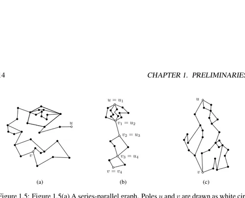
An outerplanar graph is a graph admitting an outerplanar embedding, that is, a planar embedding in which all the vertices are incident to the outer face. An outer-planar graph, together with an outerouter-planar embedding is called an outerplane graph. An outerplanar graph is maximal if all bounded faces are delimited by cycles of three vertices. From a combinatorial point of view, an outerplanar graph is a graph that con-tains no K4-minor and no K2,3-minor (see Figure 1.5(a)). Also, outerplanar graphs

1.3. FAMILIES OF PLANAR GRAPHS 13

(a)

r

(b)

(c) (d)

Figure 1.4: (a) A cycle. (b) A tree rooted at a vertex r. (c) A path. (d) An outerplane graph.

A series-parallel graph is inductively defined as follows. An edge (u, v) is a series-parallel graph with poles u and v. Denote by ui and vi the poles of a

series-parallel graph Gi. A series composition of a sequence G1, . . . , Gk of series-parallel

graphs, with k ≥ 2, is a series-parallel graph with poles u = u1and v = vk such

that vi and ui+1 have been identified, for each i = 1, . . . , k− 1 (see Figure 1.5(b)).

A parallel composition of a set G1, . . . , Gk of series-parallel graphs, with k ≥ 2, is

a series-parallel graph with poles u = u1 = · · · = uk and v = v1 = · · · = vk

(see Figure 1.5 (c)). From a combinatorial point of view, a series-parallel graph is a graph that contains no K4-minor. If follows that any (connected) subgraph of a

series-parallel graph is a series-parallel graph. Observe that outerplanar graphs are series-parallel graphs.

A graph G is a k-tree if it can be generated by a sequential addition of vertices (and their incident edges) in an order v1, . . . , vnsuch that, for each i > k, vertex vihas

ex-u v (a) u = u1 v1_{= u}2 v2_{= u}3 v3= u4 v = v4 (b) u v (c)

Figure 1.5: Figure 1.5(a) A series-parallel graph. Poles u and v are drawn as white cir-cles. Figure 1.5(b) A series composition of a sequence of four series-parallel graphs. Figure 1.5(c) A parallel composition of a set G1, G2, . . . , Gkof series-parallel graphs.

actly k predecessors (i.e, neighbors with smaller index) and they form a clique (i.e, the subgraph of G induced by the predecessors of viis the complete graph Kk). A partial

k-tree is a subgraph of a k-tree and have treewidth (i.e., the size of the largest clique in the graph) bounded by a constant. Partial k-trees received large attention since, as their treewidth is bounded by a constant, they allow for solving in polynomial time problems that are otherwise NP-hard ([AP89, CR05]). Trees coincide with 1-trees, while series-parallel graphs coincide with 2-trees. Planar 3-trees, also referred as stacked triangulations or Apollonian graphs, are special types of planar triangulations which can be generated from a triangle by a sequential addition of vertices of degree 3 inside faces. Namely, planar 3-trees can be inductively defined as follows:

• The complete graph K3on three vertices is a planar 3-tree.

• Let G be a planar 3-tree with n vertices and let a, b, and c be three vertices bounding a face of G. The graph G′ obtained by adding vertex v and edges (a, v), (b, v), and (c, v) is a planar 3-tree with n + 1 vertices.

A graph G with n ≥ 4 vertices is a wheel if it consists of a simple cycle C = (v1, . . . , nn₋₁) on (n− 1) vertices and the remaining vertex v is connected to all the

vertices of C. Wheels are triconnected graphs. The complete graph on four vertices K4is a wheel on four vertices.

1.4. DRAWING CONVENTIONS AND ÆSTHETIC CRITERIA 15

1.4

Drawing Conventions and Æsthetic Criteria

Planarity is commonly accepted as the most important aesthetic criteria a drawing should satisfy to be nice and readable. In fact, the absence of partial or complete overlapping among the vertices makes the drawing aesthetically pleasant and easily readable by the human eye, and provides extremely high readability of the combina-torial structure of the graph, as confirmed by some cognitive experiments in graph visualization [PCJ97, Pur00, PCA02, WPCM02].

However, the great importance of planar graphs, so in Graph Drawing as in Graph Theory and Computational Geometry in general, also comes from the many mathe-matical, combinatorial, and geometrical properties they exhibit.

In the following, we describe the most used drawing conventions and discuss some æsthetic criteria that characterize a good drawing of a graph.

1.4.1

Drawing Conventions

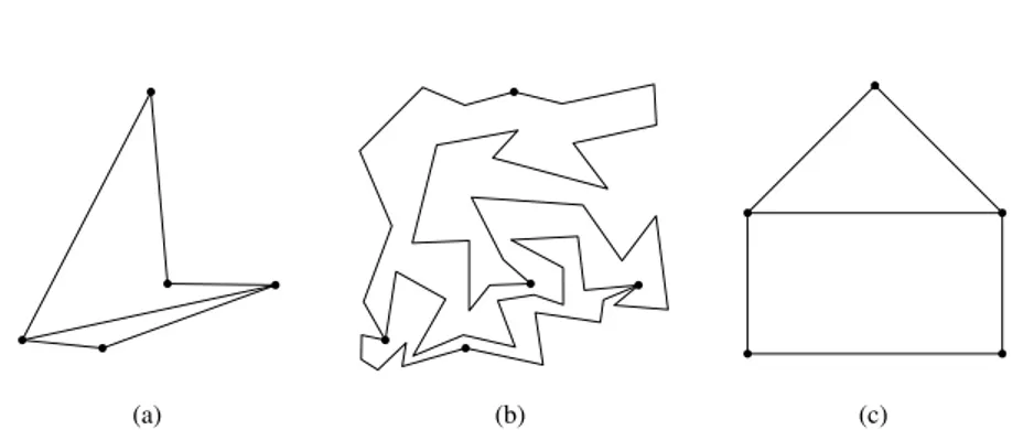
When aiming at high readability of a drawing, another important issue that has to be considered concerns the geometrical representation of the edges and of the faces. Namely, planar drawings in which edges are represented by straight-line segments (known as straight-line drawings, see Figures 1.6(a) and 1.6(c)) happen to be more readable than drawings in which edges are represented by lines (known as poly-line drawings, see Figure 1.6(b)) or general curves, and drawings in which faces are drawn as convex polygons (known as convex drawings, see Figure 1.6(c)) are more readable than drawings in which this is not the case (see Figure 1.6). Among the more used and studied drawing conventions, we also mention orthogonal drawings, in which each edge is represented by a sequence of horizontal and vertical segments.

Other drawing conventions that are worth to mention are the grid drawings, in which vertices and bends have integer coordinates, upward drawings of digraphs, in which each edge is represented by a curve monotonically-increasing in the upward direction, and proximity drawings, in which given a definition of proximity, the prox-imity graph of a set of points is the graph with a vertex for each point of the set, and with an edge between two vertices if the corresponding points satisfy the proximity property. Then, a proximity drawing of a graph G is a drawing D of G such that the proximity graph of the set of points on which the vertices of G are drawn in D co-incides with G itself. An example of proximity graphs is the Delaunay triangulation for a set P of points in the plane, that is, a triangulation T such that no point in P is inside the circumscribed circle of any triangle in T .

The most studied and used drawing convention is the one of straight-line draw-ings. Of course such a convention is much more restrictive than the one in which

(a) (b) (c)

Figure 1.6: (a) A straight-line planar drawing of a planar graph G. (b) A poly-line planar drawing of G. (c) A convex drawing of G.

edges can have bends, and hence many results that hold for poly-line drawings do not hold for straight-line drawings. However, regarding planarity, this is not the case. Indeed, a very important result, known as Fary’s theorem and independently proved by Wagner [Wag36], by Fary [F´ar48], and by Stein [Ste51], states that a graph admits a straight-line planar drawing if and only if it admits a planar drawing. This result shows that planarity does not depend on the geometry used for representing the edges but it only depends on the topological properties of the graph.

Other drawing conventions that we consider in this thesis are monotone and or-thogonal drawings. A drawing of a graph is a monotone drawing if for every pair of vertices u and v there is a path drawn from u to v that is monotone in some direction. In other words, a drawing is monotone if, for any given direction d (e.g., from left to right) and for each pair of vertices u and v, there exists a suitable rotation of the drawing for which a path from u to v becomes monotone in the direction d. Monotone drawings will be discussed in depth in Chapter 9. In orthogonal drawing, edges are represented as poly-lines composed of horizontal and vertical segments. Orthogonal drawings will be discussed and extended in Chapter 10.

1.4.2

Æsthetic Criteria

Some aesthetic criteria can be defined to measure the quality of a drawing. Among them, one of the most important is certainly the area occupied by the drawing, that is, the area of the smallest rectangle with sides parallel to the coordinate axes that contains all the drawing. Of course, small area drawings can not be obtained by sim-ply scaling down the drawing, since some resolution rules have to be respected in the

1.4. DRAWING CONVENTIONS AND ÆSTHETIC CRITERIA 17

drawing for maintaining readability. In particular, a minimum distance, say one unit, between two elements (vertices and edges) of the drawing has to be maintained. In order to respect some of such rules, when dealing with area minimization problems, vertices are usually placed on an integer grid, in such a way that the minimum dis-tance between any two of them is at least one grid unit. In this direction, it has been shown in several papers that every n-vertex plane graph admits a planar straight-line drawing on a O(n2_{) area grid [dPP88, dPP90, Sch90, CN98, ZH03, BFM07].}

Fur-ther, a grid of quadratic size is asymptotically the best possible for straight-line planar drawings, since there exist planar graphs requiring such an area in any planar grid drawing [Val81, dPP90, FP08].

Chapter 2

Data Structures for Decomposing

Planar Graphs

In order to describe and efficiently handle the decomposition of a connected graph into biconnected components and of a biconnected graph into triconnected components, some efficient data structures have been defined. In this chapter we present two such data structures, namely block-butvertex trees (bc-trees) (Section 2.1) and SPQR-trees (Section 2.2).

2.1

Block-Cutvertex Trees

The data structure that can be used to describe the decomposition of a connected graph into its biconnected components, called block-cutvertex tree (usually referred to as BC-tree), was introduced by Harary and Prins [HP66]. The BC-tree T of a connected graph G is a tree containing a B-node for each block of G and a C-node for each cutvertex of G. Edges inT connect each B-node µ to the C-nodes associated with the cutvertices belonging to the block of µ. The BC-tree of G may be thought as rooted at a specific block ν. The number of nodes ofT is equal to the number of blocks plus the number of cutvertices, that is O(n), where n is the number of vertices of G. Figure 2.1 shows a connected planar graph and its block-cutvertex tree, rooted at a block B1.

B1 B2 B3 B4 B5 B6 B7 B8 B9 B10 (a) B1 B2 B3 B4 B5 B6 B7 B8 B9 B10 (b)

Figure 2.1: (a) A connected planar graph and (b) its block-cutvertex tree, rooted at B1.

2.2

SPQR-trees

The data structure that can be used to describe the decomposition of a biconnected graph into its triconnected components, called SPQR-tree, was introduced by Di Bat-tista and Tamassia [DT90, DT96b, DT96a]. In this section we define SPQR-trees, we give their main properties, and we describe how such trees can be used to represent and efficiently handle all the embeddings of a planar biconnected graph.

In order to introduce SPQR-trees, we first give some definitions that will be use-ful in the following. A graph is st-biconnectible if adding edge (s, t) to it yields a biconnected graph. Let G be an st-biconnectible graph. A split pair{u, v} of G is either a separation pair or a pair of adjacent vertices. A maximal split component of G with respect to a split pair{u, v} (or, simply, a maximal split component of {u, v}) is either an edge (u, v) or a maximal subgraph G′of G such that G′contains u and v, and{u, v} is not a split pair of G′. A vertex w̸= u, v belongs to exactly one maximal split component of{u, v}. We call split component of {u, v} the union of any number of maximal split components of{u, v}.

Di Battista and Tamassia [DT96b] introduced SPQR-trees as rooted at one edge of G, called reference edge. However, SPQR-trees can also be viewed as unrooted

2.2. SPQR-TREES 21

since a decomposition starting from a different reference edge would yield a tree with the same structure. Here, in order to simplify the description of the construction of SPQR-trees, we only describe them as rooted trees.

Rooted SPQR-Trees

The rooted SPQR-treeTeof a biconnected graph G, with respect to a reference edge

e, describes a recursive decomposition of G induced by its split pairs. The nodes of Te are of four types: S, P, Q, and R. Their connections are called arcs, in order to

distinguish them from the edges of G.

Each node µ ofTehas an associated st-biconnectible multigraph, called the

skele-ton of µ and denoted by skel(µ). The skeleskele-ton skel(µ) shows how the children of µ, represented by “virtual edges”, are arranged into µ. The virtual edge in skel(µ) associated with a child node ν of µ, is called the virtual edge of ν in skel(µ).

For each virtual edge eiof skel(µ), recursively replace eiwith the skeleton skel(µi)

of its corresponding child µi. The subgraph of G that is obtained in this way is the

pertinent graph of µ and is denoted by pert(µ).

Given a biconnected graph G and a reference edge e = (u′, v′), treeTeis

recur-sively defined as follows. At each step, a split component G∗, a pair of vertices{u, v}, and a node ν inTeare given. A node µ corresponding to G∗is introduced inTeand

attached to its parent ν. Vertices u and v are the poles of µ and denoted by u(µ) and v(µ), respectively. The decomposition possibly recurs on some split components of G∗. At the beginning of the decomposition G∗ = G− {e}, {u, v} = {u′, v′}, and ν is a Q-node corresponding to e.

Base Case: If G∗consists of exactly one edge between u and v, then µ is a Q-node whose skeleton is G∗itself.

Parallel Case: If G∗is composed of at least two maximal split components G1, . . . , Gk

(k ≥ 2) of G with respect to {u, v}, then µ is a P-node. Graph skel(µ) consists of k parallel virtual edges between u and v, denoted by e1, . . . , ek

and corresponding to G1, . . . , Gk, respectively. The decomposition recurs on

G1, . . . , Gk, with{u, v} as pair of vertices for every graph, and with µ as parent

node.

Series Case: If G∗is composed of exactly one maximal split component of G with respect to{u, v} and if G∗has cutvertices c1, . . . , ck₋₁ (k≥ 2), appearing in

this order on a path from u to v, then µ is an S-node. Graph skel(µ) is the path e1, . . . , ek, where virtual edge eiconnects ci−1with ci(i = 2, . . . , k− 1), e1

on the split components corresponding to each of e1, e2, . . . , ek−1, ekwith µ as

parent node, and with{u, c1}, {c1, c2}, . . . , {ck−2, ck−1}, {ck−1, v} as pair of

vertices, respectively.

Rigid Case: If none of the above cases applies, the purpose of the decomposition step is that of partitioning G∗ into the minimum number of split components and recurring on each of them. We need some further definition. Given a maximal split component G′of a split pair{s, t} of G∗, a vertex w∈ G′properly belongs to G′ if w ̸= s, t. Given a split pair {s, t} of G∗, a maximal split component G′ of {s, t} is internal if neither u nor v (the poles of G∗) properly belongs to G′, external otherwise. A maximal split pair{s, t} of G∗is a split pair of G∗ that is not contained into an internal maximal split component of any other split pair{s′, t′} of G∗. Let{u1, v1}, . . . , {uk, vk} be the maximal split pairs of G∗

(k ≥ 1) and, for i = 1, . . . , k, let Gi be the union of all the internal maximal

split components of {ui, vi}. Observe that each vertex of G∗ either properly

belongs to exactly one Gior belongs to some maximal split pair{ui, vi}. Node

µ is an R-node. Graph skel(µ) is the graph obtained from G∗by replacing each subgraph Gi with the virtual edge ei between ui and vi. The decomposition

recurs on each Giwith µ as parent node and with{ui, vi} as pair of vertices.

For each node µ ofTe, we add to skel(µ) the virtual edge (u, v) representing

the parent of µ inTe. We say that an edge e′ of G projects to a virtual edge e′′ of

skel(µ), for some node µ inTe, if e′belongs to the pertinent graph of the node ofTe

corresponding to e′′. Figure 2.2 depicts a biconnected planar graph and its SPQR-tree. Property 2.1 Let C be a cycle of G and let µ be any node ofTe. Then, either the

edges of C belong to a single virtual edge of skel(µ), or they belong to a set of virtual edges that induce a cycle in skel(µ).

The SPQR-treeTe of a graph G with n vertices and m edges has m Q-nodes

and O(n) S-, P-, and R-nodes. Also, the total number of vertices of the skeletons stored at the nodes ofTeis O(n). Finally, SPQR-trees can be constructed and handled

efficiently. Namely, given a biconnected planar graph G and an edge e of G, the SPQR-treeTeof G with respect to e can be computed in linear time [GM01].

2.2.1

Drawing Plane Decomposed Graphs

In the following we give a description of how a straight-line planar drawing Γ, satisfy-ing certain properties, of a plane (biconnected) graph G can be computed by exploitsatisfy-ing its SPQR-tree Terooted at edge e.

2.2. SPQR-TREES 23 5 1 2 3 4 6 7 8 (a) S S S P P R R R 1 4 3 1 3 1 3 2 6 6 5 3 6 5 6 7 5 5 3 5 8 (b)

Figure 2.2: (a) A biconnected planar graph and (b) its SPQR-tree, rooted at any Q-node adjacent to the R-Q-node whose internal vertices are black. The skeletons of the internal R-nodes of the tree are represented inside the boxes. The virtual edge repre-senting the parent of a node µ in the skeleton of µ is drawn as a dashed line.

The drawing Γ is computed by assigning a region to each node µ of Te and

by suitably drawing the pertinent pert(µ) of µ inside such a region. The regions assigned to the nodes of Te have been introduced in [ACD+12] and [ADK+13],

and are of three types: Left boomerangs, right boomerangs, and diamonds. A left boomerang is a quadrilateral with vertices N, E, S, and W such that E is inside tri-angle△(N, S, W ), where |NE| = |SE| and |NW | = |SW | (see Figure 2.3(a)). A right boomerang is defined symmetrically, with E playing the role of W , and vice versa (see Figure 2.3(b)). A diamond is a convex quadrilateral with vertices N, E, S, and W , where |NW | = |NE| = |SW | = |SE|. Observe that a diamond con-tains a left boomerang Nl, El, Sl, Wland a right boomerang Nr, Er, Sr, Wr, where

S = Sl= Sr, N = Nl= Nr, W = Wl, and E = Er(see Figure 2.3(c)).

We assign boomerangs (either left or right, depending on the embedding of G) to S- and R-nodes, and diamonds to P- and Q-nodes. Drawing Γ is obtained by means of a top-down traversal of Te(Figures 2.3(d) and 2.3(e)), as follows.

At the first step, consider the unique child µ of the root ρ of Teand observe that,

by construction, µ cannot be a Q-node. If µ is a P-node, assign a diamond to µ. Otherwise, µ is an R-node or an S-node. In this case, assign a boomerang (either left or right, depending on the embedding of G) to µ.

At each further step, consider a node µ of Teand the region R (either a left/right

boomerang or a diamond, depending on the type of µ and the embedding of G) as-signed to it by the previous step of the algorithm. Construct a straight-line planar

S N E W (a) S N E W (b) E=Er Sl=S=Sr W =Wl Nl=N =Nr El Wr (c) S N E W C (d) E S W N C (e)

Figure 2.3: (a) A left boomerang. (b) A right boomerang. (c) A diamond. (d) Dia-monds inside a boomerang. (e) Boomerangs (and a diamond) inside a diamond.

drawing of skel(µ) in a suitable fashion that depends on the required properties of Γ in the interior of R in such a way that the poles of µ lie on points N and S of R, ac-cording to the structure of G. Then, for each virtual edge ei= (ui, vi), corresponding

to a child µiof µ in Te, assign a region Ri(either a left/right boomerang or a diamond,

depending on the type of µiand the embedding of G) to µi, in such a way that:

• uiand vilie on points Niand Siof Ri;

• Riis entirely contained in R; and

• Ri does not overlap (except possibly at points Ni and Si) with any region Rj

assigned to a child µjof µ, with j̸= i.

Then, recursively apply such a procedure to all the children of µ.

At the end of the recursive process, draw the edge e corresponding to the root ρ of Teas a straight-line segment. Observe that, by construction and by the fact that e is

Part I

Chapter 3

State of the Art

Given two straight-line planar drawings of a plane graph, a planar morph is a continu-ous transformation of the first drawing in which vertices move at uniform speed along straight-line trajectories and planarity is preserved at any time during the transforma-tion.

In this chapter we give an overview of the main works about morphing planar graph drawings. We focus on Cairns’s result, since a similar recursive approach is applied in the algorithms described in Chapters 5 and 7.

3.1

Background

Even before that most of the well-known graph drawing concepts were formalized, the problem of proving whether two drawings of the same geometric object can be trans-formed one into the other without introducing any crossings arose among researchers. To the best of our knowledge, this problem has first been studied by Tietze in 1914, who proved that two planar drawings of a polygon can be transformed into each other without introducing any crossings [Tie14]. Three years later, Smith [Smi17] simpli-fied Tietze’s proof. Also, after Steinitz [Ste16] proved that every convex polyhedron forms a triconnected planar graph, and every triconnected planar graph can be repre-sented as the graph of a convex polyhedron, Veblen [Veb17] and Alexander [Ale23] independently extended Tietze’s result to internally triconnected graphs.

In 1944 Cairns [Cai44a] focused on maximal plane graphs and gave the first al-gorithm for computing a morph of two straight-line planar drawings of such graphs by contracting a particular vertex and recursively computing a morph of the obtained (smaller) graph. Although Cairns’s algorithm requires a number of steps that is

expo-nential in the size of the input graph, it is considered a milestone in the study of this problem as it had a great impact on the approaches used to tackle the problem in the years to come. A complete description of Cairns’s algorithm is given in Sections 3.2 and 3.3.

Following this breakthrough, Bing and Starbird [BS78a, BS78b] and Ho [Ho73a, Ho73b, Ho74, Ho75], independently extended Cairns’s result in several settings in which the outer face of the graph is delimited by a convex polygon which remains fixed durign the transformation. The main idea behind these papers is that any two drawings of the same plane graph can be augmented to represent two drawings of the same internally triconnected graph.

In 1983, Thomassen [Tho83] adopted a setting defined by Gr¨unbaum and Shep-ard [GS81], i.e., in both drawings each face is delimited by a convex polygon, and, by using a contraction argument similar to Cairns’s, he proved the existence of a morph in which such convexity is maintained at any time.

Unfortunately, both Cairns’s and Thomassen’s approaches require an exponential number of steps, as they exploit a double-recursion approach and do not take into account the trajectories of contracted vertices.

In order to find an effective approach for solving the problem in the general setting, researchers decided then to focus on simpler classes of graphs or to relax some constraints. Simple polygons and trees represented then a natural input. Kent, Carlson, and Parent [KCP92], Sederberg and Greenwood [SG92], and Guibas and Hershberger [GH94], proposed the firsts algorithms for computing morphs of poly-gon in a polynomial number of steps. These results have been later improved to O(n log n) in a paper by Hershberger and Suri [HS95], in which the authors prove that the same number of steps suffices also for binary trees. Other works on mor-phing simple polygons, some of them taking into account also additional constraints are [BSW97, NMWB08, AAD+11].

Due to their structural properties, the next natural step was that of proving that a polynomial number of linear morphing steps suffices to transform drawings of plane orthogonal graphs, possibly maintaining edge orientations (as conjectured by Robin-son [Rob81] considering a setting defined by Cairns [Cai44b]). The existence of a planar morph with such properties was already proved by Thomassen [Tho83]. In this setting, it has been proven [BLS05, LPS06, Spr07, BLPS13] that if there are more than two edge directions, then the problem of finding a morph preserving such direc-tions is NP-hard, while for orthogonal drawings of plane graphs a polynomial number of steps is sufficient.

By allowing poly-line intermediate drawings, that is, “bending” the edges of the graph during the transformation, Lubiw and Petrick [LP11] found the first algorithm

3.1. BACKGROUND 29

requiring a polynomial number of moves, namely O(n6_{), coping with general plane}

graphs.

Focusing back on the original setting, the first algorithms for computing planar lin-ear morphs in O(n) moves for simple classes of graphs as paths, outerplane graphs, and plane 3-trees have been proposed in [Ros10]. Following Cairns’s approach, Alam-dari et al. [AAC+13] gave the first algorithm for morphing straight-line planar draw-ings of plane graphs that requires a polynomial number, namely O(n4), of moves. A few months later, Barrera-Cruz et al. [BHL13] gave a simpler technique for computing the motion of contracted vertices.

In this thesis we give an algorithm for morphing drawings of plane series-parallel graphs in a linear number of moves (see Chapter 5), show that Ω(n) moves are some-times necessary (see Chapter 6), and improve to O(n2) the result by Alamdari et al. (see Chapter 7). After writing this thesis, we improved the upper bound on the number of moves to O(n), thus obtaining an asymptotically optimal algorithm [ADD+14].

This problem has been studied by Angelini et al. [ACDP08, ACDP13] also in a purely topological setting. Namely, the authors study how two planar embeddings of the same biconnected graph can be morphed one into the other while minimizing the number of elementary changes.

Due to its strict relation with computer graphics animation, this problem has been studied also in the setting in which vertices can move along non-linear trajectories. The most popular approach, in this setting, is based on Tutte’s algorithm to construct planar drawings of plane triconnected graphs [Tut63], in which the vertices lying on the outer face induce a convex polygon and internal vertices are placed in the barycen-ter of the polygon induced by their neighbors. Floabarycen-ter and Gotsman [FG99] and Gots-man and Surazhsky [GS01] proved, for convex drawings of triconnected graphs, that expressing the position of each internal vertex as a convex combination of the posi-tions of its neighbors and linearly interpolating the weights of this combination be-tween the values computed in the two input drawings yields a planar morph. Surazh-sky and Gotsman [SG01, SG03] later extended this approach to triangulations and plane graphs. In this setting the main target consists in minimizing the motion of vertices having the same position in the two drawings and, when applied in com-puter graphics, the distortion introduced in intermediate drawings, hence the function used to compute the weights that are interpolated during the animation has a relevant role. During the years, many types of coordinates for expressing the positions of in-ternal vertices have been defined, some examples are [CGC+02, MBLD02, Flo03, CdVPV03, FKR05, IMH05, JMD+_07].

Finally, some tools implementing graph-morphing algorithms have been presented in [FE02, EKP03, KL08].

3.2

Overview of Cairns’s Algorithm

The algorithm proposed by Cairns [Cai44a] is a recursive process where the morph of an n-vertex maximal plane graph is reduced to two morphs of two suitable (n− 1)-vertex maximal plane graphs, as follows.

O₍₁₎ O₍₁₎ O₍₁₎ in general v′_{6= v}′′

⇒

⇒

Figure 3.1: Overview of Cairns’s Algorithm

Let Γsand Γtbe two drawings of a maximal plane graph G with n vertices such

that each of the three vertices on the outer face has the same position in both drawings, and let v be an internal vertex of G with at most five neighbors, see Figure 3.1.

First, v is removed from Γsand Γtand the resulting faces, which in general are

not convex, are triangulated in Γsand Γt. This can be done by adding dummy edges

incident to a neighbor vs(vt) of v lying on the boundary of the kernel of v in Γs(in

Γt, respectively). Observe that, in general, vs ̸= vt. Hence, two planar drawings Γσ

and Γτ of two graphs Gσand Gτwith n− 1 vertices are obtained.

Second, a drawing Γv_{of G is constructed such that: (i) both v}

sand vtlie on the

boundary of the kernel of v (for example, the polygon P induced by the neighbors of v in Γv_{is convex), and (ii) v lies in the centroid of its kernel. New drawings Γ}v

σof Gσ

and Γv

τ of Gτ are constructed from Γv by removing v and adding the missing edges

inside the polygon P , which is always possible since both vsand vthave visibility on

all the vertices of P in Γv_{, as (by construction) both v}

sand vtlie on the boundary of

the kernel of v in Γv.

3.3. DETAILED DESCRIPTION OF CAIRNS’S ALGORITHM 31

steps of Gσfrom Γσto Γvσand from a morph in h steps of Gτfrom Γvτto Γτcomputed

inductively, it is possible to construct a pseudomorph in k + h + 2 steps of G from Γs

to Γt, as follows.

The first step is used to “contract” v onto vs. The subsequent k steps are the same

as those of the morph of Gσ from Γσ to Γvσ, with v moving in accordance with its

neighbors. Since both Γv

σand Γvτhave been obtained from the same drawing Γv, the neighbors

of v have the same positions (and hence the cycle they induce is represented by the same polygon) in both drawings, vertex v can be ideally “uncontracted” from vsand

“contracted” with no additional morphing steps. In Section 3.3, we will show that the technique used to find a suitable position for v allows to reintroduce v in both Γv

σand

Γv

τin such a way that it has the same position in both drawings.

Then, the subsequent h steps are the same as those of the morph of Gτ from Γvτ

to Γτ, with v moving in accordance to its neighbors. Finally, the last step is used to

“uncontract” v from vtand to place it in its position in Γt.

Actually, in order to avoid vertex overlapping during the morph, Cairns suggests to place v in the centroid of the kernel of the polygon induced by its neighbors (instead of collapsing it onto vsand vt) and to keep it in the centroid of such a varying kernel.

However, in Section 3.4 we show that this approach might lead to non-linear mo-tion of some vertices during a single move, hence requiring several intermediate planar linear morphing steps.

3.3

Detailed Description of Cairns’s Algorithm

This section is devoted to describe in depth Algorithm Cairns Morph, that is the algorithm proposed by Cairns for morphing a planar straight-line drawing Γs of a

maximal plane graph G into another planar straight-line drawing of G. We sketch Algorithm Cairns Morph in the following.

Let Γsand Γt be two drawings of the same maximal plane graph G such that

the vertices incident to the external face have the same positions in both drawings. Algorithm Cairns Morph recursively computes a morph of Γsinto Γtas follows.

Since, by hypothesis, the three vertices incident to the external face have the same positions in both drawings, if G has no internal vertices, then there is nothing to do.

So assume that G has at least an internal vertex. By Lemma 4.7, G has an internal vertex v such that deg(v)≤ 5 (actually, in the lemma it is required that v is a candidate vertex, that is a stronger condition). Also, by Lemma 4.3, in any drawing Γ of G a neighbor x of v can be found such that x lies on the boundary of the kernel of v in Γ.

Algorithm Cairns Morph

Require: Γsand Γtare two planar drawings of a maximal plane graph G;

Γsand Γthave the same bounding polygon

/* Initialize the morphing sequence */ 1. M ← ∅

/* --- Base Case ---*/ 2. if Ghas no internal vertices then

3. return M

/* --- Recursive Step ---*/ 4. v← internal vertex of G such that deg(v) ≤ 5

5. vs← neighbor of v on the boundary of the kernel of v in Γs

6. vt← neighbor of v on the boundary of the kernel of v in Γt

7. Γv _{← drawing of G such that:}

(i) vsand vtare in the kernel of v, and

(ii) v lies in the centroid of its kernel /* Apply contractions */

8. Gσ= G/(vs)← contract v onto vsin G

9. Gτ= G/(vt)← contract v onto vtin G

10. Γσ = Γs/(v, vs)← contract v onto vsin Γs /* it’s a drawing of Gσ */ 11. Γτ = Γt/(v, vt)← contract v onto vsin Γt /* it’s a drawing of Gτ */ 12. Γv

σ = Γv/(v, vs)← contract v onto vsin Γv /* it’s a drawing of Gσ */ 13. Γv

τ = Γv/(v, vt)← contract v onto vsin Γv /* it’s a drawing of Gτ */ /* Recursive calls */

14. Mσ← Cairns Morph(Γσ, Γvσ)

15. Mτ ← Cairns Morph(Γvτ, Γτ)

/* Extend morphs Mσ and Mτ to two morphs of G */ 16. Ms← remove contraction edges and reintroduce v in each drawing of Mσ

17. Mt ← remove contraction edges and reintroduce v in each drawing of Mτ /*

Construct the actual morph M =⟨Γs, Ms, Mt, Γt⟩ */

18. M ← append(M, ⟨Γs⟩) /* M = ⟨Γs⟩ */

19. M ← append(M, Ms) /* M = ⟨Γs, . . . , Γv⟩ */ 20. M ← append(M, Mt)

21. M ← append(M, ⟨Γt⟩) /* M = ⟨Γs, . . . , Γv, . . . , Γt⟩ */ 22. return M

3.3. DETAILED DESCRIPTION OF CAIRNS’S ALGORITHM 33

Let then vsand vtbe two of the neighbors of v lying on the boundary of the kernel of

v in Γsand Γt, respectively (lines 5 and 6).

Let also Γv _{(line 7) be a drawing of G such that: (i) both v}

sand vtlie on the

boundary of the kernel of v at the same time, e.g. the polygon P induced in Γv_{by the}

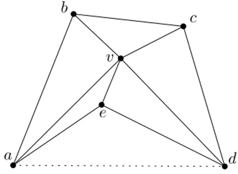
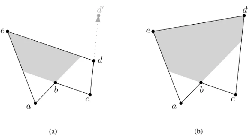
neighbors of v is convex; and (ii) v lies in the centroid of its kernel. Observe that P has not necessarily to be convex and that in some cases it cannot be drawn as a convex polygon, i.e. if an edge connecting two non-consecutive neighbors of v exists in G (see Figure 3.2).

v

a

b

c

d

e

Figure 3.2: Polygon ⟨a, b, c, d, e⟩ does not admit a convex drawing because of the external chord (a, d), drawn as a dashed segment.

In such a case, Cairns suggests to draw P “as convex as possible”. Namely, the polygon obtained from P together with its external chords is drawn convex (see Fig-ure 3.3). Note that the vertices connected by external chords cannot, in any case, lie on the boundary of the kernel of v, hence vertex v will never be contracted onto such vertices.

Since vs lies on the boundary of the kernel of v in both Γs and Γv, it can be

contracted onto vs. Let then Γσ and Γvσbe the two drawings obtained by contracting

v onto vsin Γsand Γv, respectively. Analogously, let Γτand Γvτbe the two drawings

obtained by contracting v onto vtin Γtand Γv, respectively (see Figure 3.4).

Note that both Γσand Γvσare drawings of the same graph Gσ= G/(v, vs), and the

algorithm recursively computes a morphMσtransforming Γσinto Γvσ. Analogously,

both Γτ and Γvτ are drawings of the same graph Gτ = G/(v, vt), and the algorithm

recursively computes a morphMτtransforming Γvτ into Γτ.

In order to obtain the final morph M transforming Γsinto Γt, Cairns suggests to

extend morphsMσandMτinto two morphs Msand Mtof G by first removing from

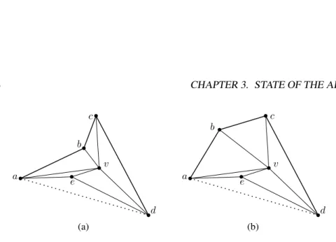
v a b c d e v a b c d e (a) (b)

Figure 3.3: (a) Polygon P =⟨a, b, c, d, e⟩ has an external chord (a, d). (b) A drawing “as convex as possible” of P : Polygon P′ =⟨a, b, c, d⟩, induced by P and its external chord (a, d), is convex. Due to the external chord (a, b), P does not admit any drawing in which a or d lie on the boundary of the kernel of v.

Γs Γt

↓ Γv _↓

↓ ↙ ↘ ↓

Γσ= Γs/(v, vs) −−−−→ Γrecursion vσ= Γv/(v, vs) Γvτ = Γv/(v, vt) −−−−→ Γrecursion τ = Γt/(v, vt)

Figure 3.4: Scheme of Algorithm Cairns Morph.

onto vt, respectively, and placing v in the centroid of its kernel in each drawing of the

two morphs.

Recall that each contraction is actually realized by moving the “contracted” vertex v to the centroid of the polygon induced by its neighbors. By the “extension” tech-nique described above, it follows that v lies in the centroid of its kernel in any drawing of both Msand Mt. Observe that the first drawing of Mtand the last drawing of Ms

are equal to Γv_{, as they are obtained by contracting v in such drawing. It follows}

that no additional morphing step is required to concatenate Ms and Mtin the final

morph M .

Also, the contraction of v onto vtand its subsequent replacement with the motion

of v to the centroid of its kernel is actually used in the opposite sense during the morph. Namely, in the last drawing of Mtevery vertex, with the exception of v, has

the same position as the one it has in Γt. In fact, in the last drawing of Msvertex v lies

in the centroid of its neighbors. Analogously, Γsand the first drawing of Msdiffer

3.4. DISCUSSION 35

Finally, morph M = ⟨Γs, . . . , Γt⟩ is obtained by the concatenation of Γs, Ms,

Mt, and Γt.

3.4

Discussion

In this section we show that the morph computed by Algorithm Cairns Morph needs an exponential number of steps and that some vertices may move along non-straight-line segments during such a morph.

3.4.1

Total Number of Moves

Let T (n) be the number of steps that compose M . The first and the last step of M move v from its initial position to the centroid of the kernel of the polygon Psinduced

by its neighbors in Γsand from the centroid of its kernel in Γtto its final position,

respectively. Such operations are realized with a single morphing step each. The remaining part of the morph is computed recursively on two smaller graphs and then extended to two morphs Msand Mtof G with no additional morphing steps. Each

of Msand Mtneeds T (n− 1) steps. The total number of steps needed by M is then

T (n) = 2T (n− 1) + 2, which gives T (n) = Θ(2n_).

3.4.2

Possible Non-linear Trajectories

In order to avoid vertex overlapping during the morph, Cairns suggests to place v in the centroid of its kernel (instead of collapsing it onto vsand vt) and to keep it in the

centroid of such a varying kernel. However, we observe that:

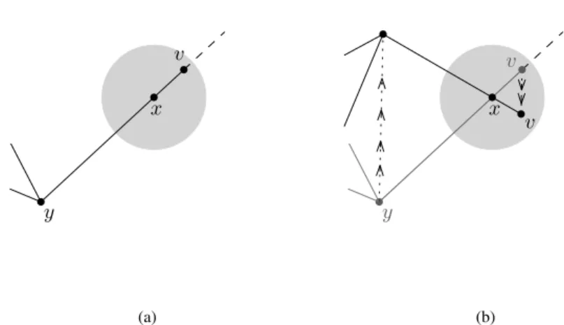
(i) since the corners of the kernel might move along curves that are not straight-line, this could result in a non-linear movement of v (see Figure 3.5);

(ii) it might happen that the number of the corners of the kernel changes during the morph (see Figure 3.6 for an example). This implies that, when the number of corners of the kernel of v changes, the position of the centroid “jumps” (namely, changes without continuity) from a point to another, thus originating a non-linear morph.