Minimal Information Exchange for Secure Image
Hash-Based Geometric Transformations Estimation
Fabrizio Guerrini, Member, IEEE, Marco Dalai, Senior Member, IEEE,
and Riccardo Leonardi, Fellow Member, IEEE
Abstract—Signal processing applications dealing with secure transmission are enjoying increasing attention lately. This paper provides some theoretical insights as well as a practical solution for transmitting a hash of an image to a central server to be compared with a reference image. The proposed solution employs a rigid image registration technique viewed in a distributed source coding perspective. In essence, it embodies a phase en-coding framework to let the decoder estimate the transformation parameters using a very modest amount of information about the original image. The problem is first cast in an ideal setting and then it is solved in a realistic scenario, giving more prominence to low computational complexity in both the transmitter and receiver, minimal hash size, and hash security. Satisfactory experimental results are reported on a standard images set.
Index Terms—Phase spectrum, secure communication, Fourier-Mellin transform, rigid image registration, distributed source coding, image hashing.
I. INTRODUCTION
T
HE need for techniques enabling the transmission of in-formation between increasingly miniaturized and energy-consumption conscious devices is tremendously accelerating, particularly due to the emergence of Industry 4.0 and IoT [1]. Their deployment is posing a series of challenges in several information technology fields, regarding, e.g., how to build and maintain device networks and associated protocols, including cloud infrastructure [2], [3], information coding paradigms [4], transmission security [5], energy harvesting and low power technologies [6], and so on.In this context, this paper focuses on the particular sce-nario that is illustrated in Fig. 1. It sits at the top-most application layer of the network infrastructure, relying on the suitable lower level device network protocols to provide raw communication facilities. An entity A has some visual information, say an image taken from a security camera at a certain time instant or an aerial/satellite image of a given location, that should be compared at a central entity B with a predetermined, locally stored copy of another version of the same visual information. The comparison could serve any one of many possible purposes, including environmental logging, Manuscript received September 13, 2019; revised February 9, 2020 and April 11, 2020; accepted April 12, 2020. Date of publication April 27, 2020; date of current version June 16, 2020. This work was supported in part by the Italian Ministry of Education under Grant PRIN 2015 D72F16000790001. The associate editor coordinating the review of this manuscript and approv- ing it for publication was Dr. Pedro Comesana. (Corresponding author: Fabrizio Guerrini.)
The authors are with the Department of Information Engineering, University of Brescia (CNIT), 25123 Brescia, Italy (e-mail: [email protected]).
Digital Object Identifier 10.1109/TIFS.2020.2990793
anomaly detection, surveillance, etc. Only B is able to perform such comparison because it has greater computational and energy resources than A, which is assumed to be little more than a sensing device, and because it is desired to limit the distribution of the data present at B.
Without imposing any additional specifications, A could transmit its image, say I, to B that compares it with its own image, say J. However, as depicted in Fig. 1, we assume that it is also desired to minimize the information knowable by a malicious eavesdropper or tamperer C, for privacy and/or other security concerns. This of course implies that both I and J must be kept secret, so A should not transmit I as plaintext, otherwise C could simply obtain it. Bandwidth is also possibly wasted as transmitting I entirely would be cumbersome.
So, this communication model needs to be further refined. Of course, a straightforward solution is easily available to address this scenario: A could encrypt its image using a private key shared with B before sending it (Fig. 2). This way, the encrypted version IK of I is of no use to C, if the
encryption is good enough, while B can decrypt it to obtain I and so perform the comparison with J in exactly the same way as in Fig. 1. This solution has two drawbacks however, both related to the assumed limits of the remote entity A. First, encryption needs computational resources that may be lacking at A (both processing power and energy consumption). Second, bandwidth is still an issue if IK has significant size,
which is at least the same as I. It is clear that some solution to save bandwidth is needed even if C were absent as in Fig. 1. Therefore, a different solution than straight cryptography alone is needed to handle this problem. In Fig. 3, instead of encryption, A performs on I some kind of message digest-ing, i.e., image hashing h(·), and transmits it. The intended objective is to give enough information about I to B to let him perform an indirect comparison between J and the hash h(I)of I. Of course, strict requirements need to be imposed on h(·). First, it must be computationally simple enough to be performed by A. Second, its possession as well as the knowledge by C of its internal operations should give as little information as possible on both I and J. In other words, only B through its knowledge of J can purposefully use h(I).
The purpose of this paper is to address the scenario proposed in Fig. 3, solving it while also minimizing the amount of transmitted information, that is the size of h(I). In doing so, it is necessary to identify in which ways I and J could differ. This can be modelled by a set of possible transformations S undergone by I to obtain J, since an universal solution is likely unattainable. Considering the applications outlined
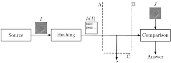
A B Source I Comparison J C Answer I
Fig. 1. Basic scenario: an entity A wants to communicate an image I to a central entity B, to compare it with a locally stored version J. I is a slightly modified version of J. However, the potential presence of an eavesdropper C prevents to send I as plaintext, plus the size of I may waste bandwidth.
A B Source I Comparison J C Answer Encryption Decryption IK I ?
Fig. 2. Revised basic scenario, taking into account the presence of C. The most obvious solution involves cryptography. In the context given by the limitations imposed upon A, however, there are obvious drawbacks because of the computational requirements on A and the size of IK.
A B Source I Comparison J C Answer ? 100111 100101... Hashing h(I)
Fig. 3. Image hashing is an acceptable compromise between the low complexity of A, sufficient security against C and bandwidth usage, while still allowing to compare h(I) with J if I is derived from J through not too strong transformations. The comparison usually requires to compute h(J) too. above, the set S should obviously include some geometric transformations, namely a mild amount of translation, rota-tion and zooming given by the unavoidably slightly different position of the camera when I and J have been captured. In addition, noise addition should be considered as well, introduced by either interpolation (assuming that I has a lower resolution than J) or the different sensors and acquisition conditions associated to I and J. Other noise sources can derive from the characteristics of the capturing camera lens, e.g., its curvature. Lastly, some local detail may be changed or missing, and detecting such occurrence could actually constitute the main purpose of the comparison.
The rest of the paper is organized as follows. Some hints on how to solve this problem can be obtained by critically analyzing some known image processing methods that for different reasons are related to the proposed application, specifically including image registration, content hashing and distributed source coding. In Sec. II they are broadly reviewed, of course limiting the scope to what is actually useful in the context of this paper, while providing the necessary motiva-tions underlying the methodology that we selected to solve the proposed application scenario. Then, Sec. III provides some notations while exploring the ideal case of noiseless, circular shifts. Sec. IV discusses the modifications that are needed
in a realistic scenario while also extending the framework to scaling and rotations. Sec. V provides some experimental results and discussion and finally Sec. VI concludes the paper.
II. RELATEDWORK ANDCONTRIBUTIONS
This section provides a wide though brief overview of the techniques most pertinent to the application problem at hand, covering several different image processing methods, to moti-vate the structure of the solution presented later in the paper. Comparing two similar images and estimating the parame-ters of the transformation allowing to obtain the second image starting from the first embodies a reference problem for this paper. Matching of visual data, e.g., 2-D images, that represent the same scene taken at different viewing conditions, with different sensors and/or at different times, is referred to as image registration [7]. In many cases, the problem is modelled by assuming that some kind of transformation is applied to the source image to obtain the target one, as we did in Sec. I with the set S. The objective is usually the estimation of the registration parameters of the transformation, allowing to find the relation between the coordinates of both images’ pixels.
The study of image registration techniques has a long tradi-tion. Rigid image registration is the most traditional instance in which the second image is obtained from the first by means of an affine transformation, or specifically enforcing a similarity geometric relation, i.e., translation, rotation and/or scaling and not shearing, and it is the most relevant for this paper. In this case the (planar) relation between the pixels of the first image (r1, c1)and those of the second image (r2, c2)is represented
by the following equation: 2 4 rc22 1 3 5 = 2
4 cos(✓sin(✓00)) cos(✓sin(✓00)) mmrc
0 0 1 3 5 · 2 4 rc11 1 3 5 (1) where is the scaling factor, ✓0 represents the rotation,
and [mr, mc] is the translation (or shift) vector. Shearing is
excluded by the zeroes in the last row. Rigid image registration as in Eq. (1) has a long history, of which [8], [9] represent early examples. Despite steady progress [7], [10], robust image registration is still a very active area of research in the most challenging scenarios outlined in what follows.
Depending on the particular application, the requirements imposed on image registration may widely change, due to the different conditions on the estimated registration parameters. For example, in remote sensing [11] it is usually required to match pairs of satellite images, taken from different viewing angles and at different times, compensating for a variety of distortions and noise sources, e.g., landscape changes. Instead, medical image registration [12] is useful to fuse images from different acquisition devices, to study anatomic or organs evolution in time and to estimate variations across subjects.
In both these application fields, image registration could also be called co-registration because, differently from the scenario proposed in this paper, the source images (I and J) are in fact both fully available. The difficulty in these registration contexts lies in the fact that they usually have to deal with non-rigid image registration [13], that is enabling the handling of elastic deformations of the source images in addition to
geometric transformations. It is notable that even in these cases global or local rigid image registration is still sometimes needed, possibly after the images have been resampled and projected on a common planar frame of reference, as the most recent literature shows (see [14]–[17], to name a few).
Limiting the scope to the classic literature on rigid image (co-)registration, the most useful paradigm for our purpose is certainly phase-based registration, that is based on the shifting property of the DFT. Extensions to the standard Fourier trans-form, e.g., the Fourier-Mellin transtrans-form, allow to formulate all kinds of affine transformations while still adopting a phase-based registration framework [18], [19]. There exist other popular approaches, e.g., [14], [20], that however usually rely on some sort of sophisticated feature extraction and matching. To summarize so far, DFT phase correlating techniques are among the most reliable whilst being computationally light in rigid image registration, when the latter is performed on a pair of available images. In the scenario depicted in Fig. 3, instead, it is assumed that only a hash of one of the source image is available, which is in essence a compact description of its content, whose extraction we discuss next.
Concise content representation, sought to be invariant under a certain class of transformations, is another relevant problem in image processing (and in audio and video processing as well), garnering decades-long attention in the research community. Depending on the intended application and the features they are based on, content representation techniques have been variably called. For example, the techniques under the ‘content hashing’ umbrella term have been first introduced as methods akin to cryptographic hashes as a way to facilitate content indexing and retrieval [21]. The name hashing has been subsequently carried over to copyright enforcing authen-tication and other security based applications [22]–[24]. In these contexts the term robustness is always introduced to signify the invariance of the content descriptor with respect to a number of manipulations interpreted as non-malicious, to which (affine) geometric transformations usually belong [25], [26] (when they are not purposefully and maliciously magnified to exploit a system weakness). The term content digest is also sometimes used [27], in particular when it is instead intended to emphasize the fragility of the content descriptor, a characteristic shared with message digests used for cryptography. Sometimes, robust hashing techniques have been called fingerprinting with the same meaning, both for images [28], video [29], and especially audio [30], notably for copyright-related content identification, e.g., the current ContentID technology employed by the popular YouTube video sharing service. On the other hand, recently the term fingerprint is also used in forensics to authenticate content creating devices [31], instead of the content itself.
In all of these content representation techniques, there is, among many others, a key discriminant parameter that allows one to clearly separate them in different classes, that is the presence, during the analysis stage, of the reference image. When it is missing, they are usually called blind techniques; when it is present, the term non-blind techniques applies; and sometimes, the name semi-blind techniques is used for the availability of partial information on the reference image. For
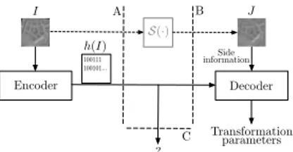
A B I J Encoder 100111 100101... Decoder S(·) Side information h(I) parameters Transformation C ?
Fig. 4. In this scheme Fig. 3 is revised consistently with DSC nomenclature, so that the image J actually embodies the side information at the decoder.
example, consider image forensics [32], where the objective is usually to assess whether a supposedly forged image, or a part of it, has been obtained from an unknown original image, e.g., through affine transformations or compression. In this case the source image is actually unknown, that is why this application can in fact be referred to as blind image forensics [33]. Classic co-registration discussed earlier, on the other hand, may be classified as non-blind since both images are available during the comparison. In contrast, hash-based techniques such as ContentID deal with partial information. In this paper the proposed technique belongs to the latter category, since the transmitted reference image information is carried by the partial information represented by the image hash.
From the analysis carried on so far, we can conclude that no image registration or forensics technique is directly applicable to our case because we follow a semi-blind paradigm. On the other hand, the robust image hashing or fingerprinting techniques for content authentication cited above, while pro-viding partial information as desired, strive for hash robustness with respect to the set S and are therefore unsuitable for our purposes (the transformation estimation) since they are designed with a completely different objective in mind. To the authors’ knowledge, no image hashing technique has ever targeted the transformation undergone by the image instead of its content.
The approach followed here is that the particular problem depicted in Fig. 3 can be solved casting it in a Distributed Source Coding (DSC) scenario [34], even if the intended application does not belong to the kind of those traditionally invoked when strictly employing distributed source coding, such as for example multi-camera image coding and compres-sion [35]. As a matter of fact, DSC notions have already been proposed for image hashing, in particular the joint application of DSC and compressive sensing [36] has been employed to extract a robust hash for semi-blind image authentication and tamper detection [37]. The proposed solution is an image hash extraction technique, inspired from the aforementioned DFT phase-based co-registration paradigm, as a framework to estimate the registration parameter at the decoder, and exploiting DSC to handle the partial information transmitted by the capturing device treating it as the decoder input.
Therefore, Fig. 3 is revised to Fig. 4 to make it adhere to the DSC scenario as proposed. Here, the encoder (the capturing device A) has to communicate the image I to the decoder (B) using the target image J as side information. In other words, the decoder knows the transformed image J = S(I),
where S(·) belongs to S, and the encoder needs to send some information connected to the registration parameters, that we still refer to as h(I) and is in effect the image hash, though targeted to the undergone transformation. The hash should be the most compact possible and allow the decoder correctly reconstruct I by inverting the estimated S(·). Thus, as discussed in the next section, the problem considered in this paper is how to build such image hash. We refer to this question as the minimal information registration problem, and in essence it will be shown in the following to correspond to a shift encoding problem, that is how to encode the phase shifts to let the phase-based registration technique to take place at the decoder, with the minimal amount of transmitted information. The contribution of this paper is thus twofold. Given that the proposed hash strives for minimal hash length, the technique description follows a bottom-up approach, starting from an ideal case requiring very few bits and building upon them to reach more realistic scenarios. Its first objective is thus to revise the theoretical background in the ideal case of noiseless, circular shifts, providing bounds for the scenario of Fig. 4, in the process answering to the crucial theoretical question on how much information about the original image in the ideal case is necessary to correctly recover the rigid transformation parameters, given the distorted image.
In a realistic environment, the global rigid geometric trans-formations that are targeted by the proposed hash are not the only modifications potentially occurring to I. In fact, phase encoding is best suited to achieve robustness against said transformations, while being fragile to excessive applica-tion of any other modificaapplica-tion. In particular, local estimaapplica-tion of non-rigid transformations as usually performed in co-registration, such as an object elastic deformation, cannot be achieved, given the fact that the proposed hash is akin to a global descriptor (though we will extend it to perform local comparisons in Sec. V-C). Instead, object (local) non-rigid transformations represent a noise source for the estimation of global geometric transformations. Also, non-rigid global transformations cannot be estimated using the DFT shifting phase is not feasible. As a consequence, some experimental results on a representative image set are reported that deal with a variety of disturbances for the geometric transformations estimation process that are significant in the context depicted by Fig. 4. They include Gaussian noise addition to address noisy image capturing, patch modifications to simulate small objects entering or leaving the scene as well as radically changing their appearance (e.g., by turning, thus including local rigid deformations), and global photometric and non-rigid transformations induced by different conditions and/or shortcomings in the camera lenses used at A (for example, radial distortion). The results are critically compared with traditional feature-based registration to highlight how compact and computationally simple the hash h(I) actually is.
The second objective of this paper is to show the develop-ment of the proposed shift encoding framework for real images using a reasonable set of registration parameters pertaining to geometric transformations in the presence of the just discussed noise sources, while also discussing its security features. The proposed hash, even if it is very few bits long, is proved to
be clearly useful as a building block in more complex appli-cations involving more challenging transformations, either to be estimated or to be robust against (if A can afford it).
III. IDEAL CASE:CIRCULAR SHIFTS
Here, the shift encoding problem is introduced starting from the ideal case of circular shifts, extending the preliminary study in [38]. This is of course an unrealistic assumption when dealing with the proposed scenario or even rigid image registration. In Sec. III-A the problem is introduced in the 1-D case and it is then extended to the 2-D case in Sec. III-B. A. Horizontal shifts: the 1-D case
First, let us restrict the set of transformations S(·) to just horizontal circular shifting, i.e., the image I is circularly shifted in the horizontal direction to obtain J. The problem is reduced to the analysis of a single pair of matching rows of I and J. In fact, it will be apparent that the analysis of just one row of the images is sufficient to correctly solve this instance of the minimal information registration problem (as long as it conveys meaningful phase information). To be consistent with the typical DSC nomenclature, let us refer to the row of the source image I as x[n] and to the corresponding one in the reference image J as y[n]. Thus, let us assume there are a pair of (row) sequences x[n], n = 0, . . . , N 1 and y[n], n = 0, . . . , N 1, and that y[n] is a circularly shifted version of x[n] by m samples, that is x[n] = y[(n m)N],
where (·)N is the modulo N operation. Let us also assume that
0 m < M < N, both N and M are powers of 2, and m is uniformly distributed in [0, M 1]. No further prior information on the shape or features of x[n] is assumed as known.
The minimal information registration problem in an ideal setting for 1-D sequences is stated as follows: what is the minimum amount of information about x[n] that is needed to correctly estimate the shift m, given y[n]? Of course, if x[n] is also given (as would happen in a co-registration scenario) the problem is trivial, since to obtain m the straightforward solution is to directly inspect the samples’ position (or alter-natively to compute the circular cross-correlation between the sequences). On the other hand, knowing only y[n] the problem is unsolvable unless some prior model on x[n] is assumed, such as the distribution of its frequency-domain coefficients and/or the knowledge of some boundary conditions.
Casting the problem in the DSC scenario depicted in Fig. 4, the encoder has to communicate x[n] (coding it in some way) to the decoder using the target sequence y[n] as side information. In the limit case, if y[n] were known not just to the decoder but also to the encoder, the latter would just have to send the value of m, so log(M) bits would be sufficient to encode x[n]1. It can be proven that log(M) bits are all that
is needed even in the case of Fig. 4, that is when the encoder does not know y[n], whose proof is briefly summarized next. Using the DFT phase-based registration paradigm men-tioned in Sec. II, let X[k], Y [k] respectively be the DFT of x[n], y[n] and X[k], Y[k]be the phase of the DFTs X[k],
1Note that log(·) is always intended as log
Y [k]. Since y[n] is a circularly shifted version of x[n], their DFTs have the same magnitude. The shifting property of the DFT dictates for the phase:
X[k] 2⇡ = Y[k] 2⇡mk N (2) where 2⇡
= means 2⇡ congruence. Ideally, it is possible to estimate m by observing just a pair of non-zero DFT samples’ phase { X[j], Y[j]}, as long as j 6= 0. For example, for
j = 1 Eq. (2) becomes: X[1] 2⇡ = Y[1] 2⇡ m N (3)
Therefore the phase difference between X[1] and Y [1] is the m-th multiple of 2⇡/N. Knowing Y[1], to identify X[1]with the least amount of information the latter can be
quantized into N values, each identifying a separate 2⇡/N phase interval, obtaining ˆX[1]. However, given that m < M,
the decoder actually needs to know only Y[1]and (ˆX[1])M
to reconstruct X[1], so the amount of information sent by the
encoder is still just log(M) bits and not log(N).
Quite interestingly, the solution to this problem is not unique. Instead of finely quantize a single phase value, the same result can be obtained using a coarser, 1-bit quantization of the phase of log(M) DFT coefficients. Although there is no difference from a theoretical point of view, since the amount of information needed at the decoder is still log(M) bits, in the practical scenario that we tackle next, this new strategy has clear benefits for robustness purposes. So, instead of taking a single phase value, let us consider log(M) phase values taken at exponentially spaced positions:
X N 2 , X N 4 , X N 8 , . . . , X N M (4)
that is, X[2 iN/2] with i = 0, . . . , log(M) 1. The
shift m can be represented by a binary representation {mQ, mQ 1, . . . , m1, m0}, with Q = log(M) 1. Each
bit can be determined by looking iteratively at each of the
X[2 iN/2]in turn, as it is now proven by induction.
Starting with the base case, i.e., the LSB m0, substituting
k = N/2(the position corresponding to i=0) in Eq. (2) gives:
X N 2 2⇡ = Y N 2 ⇡m 2⇡ = Y N 2 ⇡m0 (5)
since the other bits of m contribute integer multiples of 2⇡. Therefore the 1-bit information associated to the sign of X[N/2] is enough to recover m0. Now, the inductive
hypothesis is that mh 1, mh 2, . . . , m0have been identified
using the signs of X[N/2], X[N/22], . . . , X[N/2h]. For
the coefficient in k = N/2h+1, Eq. (2) now gives: X N 2h+1 2⇡ = Y N 2h+1 ⇡ m 2h 2⇡ = Y N 2h+1 ⇡mh h (6) Since the most significant bits {mQ, mQ 1, . . . , mh+1} all
contribute integer multiples of 2⇡ and the decoder can compute the term h = ⇡/2h{mh 1, mh 2, . . . , m0}, the sign of X[N/2h+1] uniquely determines mh. Therefore, the signs
of X[2 iN/2] build the hash h(I), as they allow to extract
the log(M) bits needed to represent the shift m.
Notably, the coefficients selected by Eq. (4) do not include
X[1]. Since just log(M) bits are necessary, the derivation
that has been proposed above begins at N/2 for the LSB and ends at N/M 6= 1 for the MSB.
B. Generic shifts: the 2-D case
We now consider the case where the N ⇥ N image J is a circularly shifted version of I using a two-dimensional shift vector m = (mr, mc), still assuming that 0 mr < R and
0 mc < C, with R < N and C < N powers of 2. To
extend the results presented in Sec. III-A, let us refer to the images I, J as the matrices x[r, c], y[r, c], respectively. Thus: x[r, c] = y[(r mr)N, (c mc)N], r, c = 0, 1, . . . , N 1 (7)
The relation between the phase of the 2-D DFT coefficients X[k, l] and Y [k, l] is:
X[k, l]2⇡= Y[k, l] 2⇡mrk
N
2⇡mcl
N (8)
By imposing respectively l = 0 and k = 0, the problem of determining mr and mc becomes separable. Therefore, mr
and mccan be encoded separately using the method presented
for the 1-D case twice, i.e., by extracting the signs of the following phase coefficients:
X N 2, 0 , X N 4 , 0 , X N 8, 0 , . . . , X N R, 0 X 0,N 2 , X 0,N 4 , X 0,N 8 , . . . , X 0,N C (9) Hence, the ideal case pertaining to 2-D circular shifts is solved in the same exact way as in the 1-D case and the total information needed to encode the shift vector is thus log(R) + log(C) bits. For example, if R = C = 27, 14 bits
are necessary for h(I).
IV. THE MINIMAL INFORMATION REGISTRATION PROBLEM IN A REALISTIC SCENARIO
In a more realistic scenario, the images I and J are cropped views of a common scene. Thus, the shift between the images can no more be modelled as circular, and border effects are introduced. In addition, to complete the framework there are additional noise sources to contend with, for example due to grid resampling and differences in capturing devices, or some local details changing. Under these assumptions, using just log(R) + log(C) bits to encode the shift in the hash of I is not reasonable. Instead, more bits will be needed as the noise strength increases. Of course, now the maximum shifts in the horizontal and vertical direction must be limited to let the overlap between the matrices x[r, c] and y[r, c] representing the images to be sufficient to recover the shift vector m. In this section we propose a robust strategy to recover m encoding the phase shifts using a small enough number of bits.
In the end, the data encoded in h(I) needs some form of redundancy to be robust against noise, akin to a channel code. Referring to the ideal case covered in Sec. III, we proved that such problem is separable and we can solve for mr and mc by substituting respectively l = 0 and k = 0 in
0 2 4 8 16 32 64 0 2 4 8 16 32 64 Z X X X X X X X X X X X X X X Y Y Y Y Y Y Y Y Y Y Y Y Y Y Y Y Y Y Y Y Y Y Y Y Y Y Y Y Y Y Y Y Y Y Y Y Y Y Y Y Y Y Y Y Y Y Y Y Y Y Y Y Y Y Y Y kl Y Y Y Y Y Y Y Y Y Y Y Y Y Y Y Y Y Y X X Y Y Y Y Y Y Y Y Y 512 256 128 128 256 512
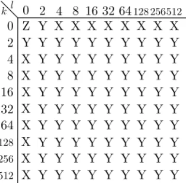
Fig. 5. The 2-D “sub-frequency” domain is illustrated in matrix form, for R = C = 256and N = 1024. The k and l indices span logarithmically spaced positions from 0 to N/2. The Z bit (DC coefficient) does not bear phase information and therefore it is never considered. The X bits, corresponding to the k = 0 row and l = 0 column, are the log(R) + log(C) = 16 bits indicated by Eq. (9), used for the ideal case. The lowest index in Eq. (9) is thus N/R = N/C = 4. To increase robustness, k = 2 and l = 2 are added to the ranges and “diagonal” frequencies are also considered, as depicted by the Y bits. Therefore, if the positions given by the whole sub-frequency matrix are encoded, the hash is (log(R) + 2) · (log(C) + 2) 1 = 99 bits long. Eq. (8). If instead we consider the coefficients with l, k 6= 0, the resulting phase difference of the matching DFT coeffi-cients depends on both mr and mc. Therefore, considering
“diagonal” frequency phases X[2 iN/2, 2 jN/2]is a sort of
“parity check” for the phase differences, that can be exploited to increase the robustness against the noise. In addition, the logarithmically spaced positions that span k =2, . . . , N/(2R) and l =2, . . . , N/(2C) when N >2R and N >2C, which are not necessary in the ideal case of Eq. (9) as they are redundant, can be used as well. In Fig. 5 there is a depiction of the strategy for increasing robustness, for the case of R = C = 256 and N = 1024. The k and l values considered in this case are those exponentially spaced as in Eq. (9), with the addition of k = N/(2R) = 2 and l = N/(2C) = 2. Of course, the hash length depends on the choice of R and C, that in turn are limited by N and M. Hash robustness is proportional to its length, maximized by choosing R = 2blog (N)c 1 and
C = 2blog (M)c 1and using all diagonal frequencies.
The decoding technique in this case is more complex, and it is similar to minimum distance decoding for channel codes. In particular, let us consider the bits extracted from the DFT phases of X[k, l] as the image hash h(I), which is sent to the decoder. All possible shift vectors (in a given range dictated by S) are applied by the decoder to the side information, the image J (that is, its DFT Y [k, l]) and the corresponding hash h(J) is extracted. The most likely shift that was applied to x[r, c] to obtain y[r, c] (the opposite of that applied to Y [k, l] in the decoding procedure) is declared as the one where the hashes h(I) and h(J) are most similar.
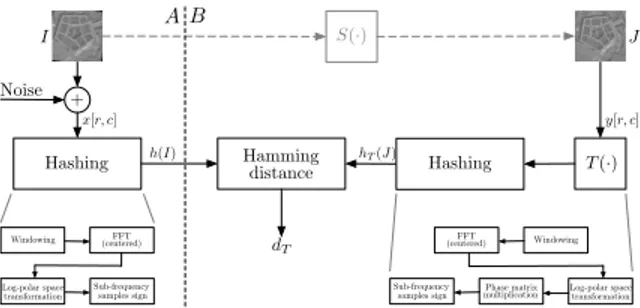
In detail, the processing stages are illustrated in Fig. 6. Let us suppose that J = S(I), where S 2 S, and in this case J is obtained through a shift of I. Some noise is possibly added to I before the hash h(I) is computed. The hash extraction is then performed on the matrices x[r, c] and y[r, c], corresponding to I and J, at the encoder and decoder side respectively. The decoder computes a hash hT(J) for
every possible transformation T (·) in S, or a suitable superset
+
Hashing Noise
Windowing FFT Sub-frequencysamples sign I h(I) x[r, c] Hashing Windowing FFT Sub-frequency samples sign multiplicationPhase matrix Hamming distance dT T (·) S(·) J hT(J) y[r, c] A B
Fig. 6. The flowchart depiction of the proposed algorithm for the hashes extraction and comparison. The B side (at the decoder) is repeated for every possible transformation T (·), in this case shifting in the image domain, to search for the one giving the minimum distance.
thereof: in this case, for every possible shift in a suitable range in the image domain. Comparing every hT(J) with the hash
h(I) transmitted by the encoder outputs a distance dT. The
transformation ˆT giving the minimum distance dTˆ provides
an estimation of S(·) by declaring S(·) = ˆT 1(
·).
The hash extraction at both sides proceeds as follows. To keep the decoding process simple, the transformation T (·) is not actually applied to J prior to the computation of h(J). Instead, its effect is simulated in the frequency domain, therefore integrating it directly in the hash extraction process. First, since x[r, c] and y[r, c], even after the shift compensation that follows, can only coincide in the central part due to border effects, applying smoothing windows on them is advisable. Then, the FFT is computed on both windowed matrices.
Next, since each T (·) is actually a shift in the image domain, at the decoder for the corresponding shift vector a compensation term is subtracted to the phase of the DFT coefficients as in Eq. (8), by multiplying the DFT matrix with a suitable phase matrix. Therefore, windowing is employed on y[r, c] just once before applying the shift to the DFT matrix. Also, just a submatrix of the DFT coefficients is considered at both sides, i.e., the subset of those exponentially spaced as in Eq. (9). The shift compensation operation actually applies a circular shift in the “sub-frequency” domain of Y [k, l]. The hashes h(I) and hT(J) are finally obtained as
the sign of the DFT phases at the selected sub-frequencies. The Hamming distance is employed to compute dT, and the
pair (h(I), hTˆ(J))with the minimum dTˆ is searched for.
To increase robustness, or equivalently to reduce the number of bits for a same noise strength, it is possible to increase the computational complexity of the decoder. In particular, windowing the image after (instead of before) each shift vector is applied to Y [k, l] greatly reduces the border effects. The computational price to pay is high since the 2-D DFT of the transformed Y [k, l] must be calculated anew for each considered shift vector. In the experiments, to be conservative we used the lighter, less robust version of the decoder, since it is assumed that many encoders (i.e., capturing devices com-municating with B) can be present, and so it is more important to free up as many computational resources as possible at the decoder side too than to further increase decoding precision. A. Extension to rotations and scaling
As we mentioned in Sec. II, the minimal information registra-tion problem when also dealing with scaling and rotaregistra-tion may
+ Hashing Noise Windowing FFT (centered) Log-polar space transformation Sub-frequency samples sign I h(I) x[r, c] Hashing Windowing FFT (centered) Log-polar space transformation Sub-frequency samples sign Phase matrix multiplication Hamming distance T (·) S(·) J hT(J) dT y[r, c] A B
Fig. 7. In case T (·) consists of scaling and rotation, the following flowchart applies instead of the one in Fig. 6. In case translation in the image domain is also considered, that procedure is applied after this one first estimates scaling and rotation and the so determined transformation is inverted.
still be solved as shift encoding in a suitable domain, namely the Fourier-Mellin transform. First, let us briefly recap how this transform is exploited in the registration context.
For simplicity sake, let us assume first that x(u, v) and y(u, v) are noiseless, continuous-domain 2-D signals, and y(u, v)is derived from x(u, v) through a translation by a shift vector m = (mr, mc), rotation by an angle ✓0and scaling by
a factor . Therefore:
x(u, v) = y( (u cos ✓0+ v sin ✓0) mr,
( u sin ✓0+ v cos ✓0) mc)
(10) which is equivalent to Eq. (1) for continuous signals. The continuous-domain Fourier transform of Eq. (10) is:
ˆ X(k, l) = e j m(k,l) 2 Y (ˆ 1(k cos ✓ 0+ l sin ✓0), 1( k sin ✓ 0+ l cos ✓0)) (11) where (k, l) are now real-valued as well and m(k, l)indicates
the phase term given by the translation m. Casting the Fourier transformed signals in log-polar coordinates, we can compute:
¯
X(⇢, ✓) =| ˆX(e⇢cos ✓, e⇢sin ✓)| ¯
Y (⇢, ✓) =| ˆY (e⇢cos ✓, e⇢sin ✓)| (12) and using Eq. (11) we have:
¯
X(⇢, ✓) = 12Y (⇢¯ ln( ), ✓ ✓0) (13)
So, the already discussed shift encoding technique can be used in this context as well to let the decoder retrieve the scale and rotation parameters. Note that Eq. (13) does not depend on m, i.e., the shift vector in the image domain.
However, this procedure holds rigorously just in the ideal case of infinite support, continuous domain images. The pre-viously stated considerations about the application on real images still apply, in particular windowing is doubly important in the log-polar domain since most of the spectrum lies close to the ⇢ = 0 axis. In addition, since only integer coordinates are valid for digital images, ln( ) in Eq. (13) can be recovered only to the nearest integer value. Thus, it is better to use a small base µ for the logarithmic resampling instead of e, so that the powers of µ are dense enough around 1, where reside typical values of for the most reasonable choices for S.
Fig. 7 describes in detail the proposed solution for the minimal information registration problem for the scaling and
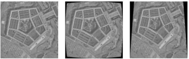
Fig. 8. The dataset is a mixture of classic images such as Cameraman on the left, satellite images such as Pentagon in the left middle, and environmental outdoor images such as Walkbridge and one image from [39] on the right. rotation case. The framework is similar to that illustrated by Fig. 6, but this time the frequency domain is cast in the log-polar space before taking the sign of the samples at the selected sub-frequencies to build the hashes. Note that the FFT must be centered around the origin so that the log-polar transform covers the appropriate region of the parameter space (⇢, ✓).
The above procedure allows to estimate the rotation and scaling parameters only. In case a shift in the image domain is simultaneously applied, it is also necessary to estimate the spatial shift m = (mr, mc). To do that, first the scaling
and rotation transformations are undone by applying to J the inverse transformation (that is, using the estimated 1
and ✓0 in Eq. (1)). Note that such operation is in principle
independent from the applied shift m, as long as border effects do not count too much. Then, the shift vector can be recovered by applying the procedure explained for the registration problem in presence of just image translation explained by Fig. 6. Of course, some caution is needed during the inverse transformation to ensure that it is applied in the same coordinate system as the applied direct transformation, which is thus variable with each shift tested at the decoder.
V. EXPERIMENTALRESULTS
Several experiments have been conducted to ascertain different properties of the proposed methodology. First, the estimation accuracy relative to the transformation parameters is evaluated. The processing chain of Fig. 6 corresponding to the shifting in the image domain and that of Fig. 7 for rotations and scaling are separately simulated and tested, with and without added Gaussian noise. Then, those chains are employed in series and the overall performance is evaluated for the case where both transformation classes are simultaneously applied as well. The accuracy performance is also assessed even when some image content modification has taken place, in this case by modifying an image patch of variable size and shape. An extension to the basic hash is also proposed to aid in localizing the modified patch once the geometric transformation has been estimated and inverted at the decoder. Next, robustness against global non-rigid and photometric transformations is assessed, for the radial distortion, view angle change, and contrast adjustment and Gaussian blurring cases. To put the proposed method in perspective from an application standpoint, its performance is also compared with that of state-of-the-art, local features based matching techniques. Last, some more results pertaining to the security (at the application level) are presented.
The experimental dataset is a collection of 75 grayscale, 512⇥512 images (a subset is depicted in Fig. 8), 15 of which are taken from well-known image repositories such as [40] and
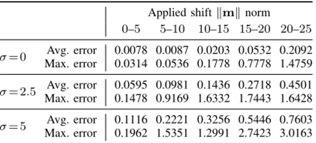
TABLE I
SHIFT ENCODING PERFORMANCE FOR TRANSLATIONS.
Applied shift kmk norm 0–5 5–10 10–15 15–20 20–25 = 0 Max. errorAvg. error 0.0078 0.0087 0.0203 0.0532 0.20920.0314 0.0536 0.1778 0.7778 1.4759 = 2.5 Max. errorAvg. error 0.0595 0.0981 0.1436 0.2718 0.45010.1478 0.9169 1.6332 1.7443 1.6428 = 5 Max. errorAvg. error 0.1116 0.2221 0.3256 0.5446 0.76030.1962 1.5351 1.2991 2.7423 3.0163
the others are a selection of outdoor images from the dataset employed for [39]. They have been chosen to represent a well balanced representation of the potential applications of the proposed techniques. In all experiments, the transformation parameters are searched for in a range 50% wider than the ground-truth ones. The experiments are run encoding the same number of bits: R and C are set to 2blog (512)c 1 = 256
for maximum robustness and the phase is thus to be probed in log(256) = 8 exponentially spaced positions (see Fig. 5). In the proposed application, more accuracy and robustness is surely desired at the expense of the hash length, given that it is already very small even in its more conservative configuration. Therefore, to increase robustness the sub-frequency matrix is encoded using all diagonal frequencies down to k = 2, thus requiring 80 (8 + 8 + 8 · 8) bits of transmitted information for each hash. Zero-mean, white Gaussian noise with variance
2is added to the received images for experiments involving
noise addition. Each experimental result involving noise addi-tion is averaged over 100 noise realizaaddi-tions. The noise can be indifferently added to either X or Y : we selected the former because it leads to a faster implementation of the experiments since this way the hash of X is computed only once per run (see Figs. 6–7). As for the windowing process, which is in common to both processing chains, the Tukey window is applied on the whole image with the parameter r = 0.9. Just the cropped, central R⇥C = 256⇥256 portion of the image is considered to build the hashes, as previously mentioned.
As a note on computational complexity at the receiver, for a 512⇥512 image, the decoding algorithm implemented in MatlabR on a sub-standard desktop computer takes on
average just 0.126s to estimate the shift parameters in the image domain, and 0.132s in the log-polar domain. The hash extraction times are given in Sec. V-E.
A. Accuracy with respect to combined rigid transformations First, we considered integer shifts directly in the image domain in a [ 20, 20] range for both the horizontal and vertical directions, giving a total of 412 1 = 1680 tested shifts.
The shifting transformation has been applied without cropping, letting the successive windowing process to take care of the zero-padded boundaries. The results are shown in Table I. Each value in the table gives the average of the norm of the error between the estimated and the ground-truth shifts in a given interval of the applied shift vector norm, given in pixel units. For example, the first column of the table
TABLE II
SHIFT ENCODING PERFORMANCE FOR SCALING.
Recovered scaling error ⇢err(%) 0–1 1–2 2–3 3–4 4–5 5–6 > 6 ⇢ = 1.02, = 0 0.847 0.145 0.002 0.002 0.002 0 0.001 ⇢ = 1.02, = 5 0.831 0.149 0.005 0.003 0.001 0.002 0.005 ⇢ = 1.08, = 0 0.884 0.070 0.011 0.017 0.006 0.002 0.006 ⇢ = 1.08, = 5 0.816 0.084 0.018 0.008 0.014 0.003 0.007 ⇢ = 1.14, = 0 0.746 0.178 0.018 0.019 0.009 0.013 0.002 ⇢ = 1.14, = 5 0.677 0.215 0.029 0.022 0.014 0.016 0.019 ⇢ = 1.20, = 0 0.657 0.180 0.038 0.029 0.006 0.011 0.078 ⇢ = 1.20, = 5 0.638 0.199 0.040 0.033 0.013 0.015 0.068 TABLE III
SHIFT ENCODING PERFORMANCE FOR ROTATION.
Recovered rotation error ✓err( ) 0–1 1–2 2–3 3–4 4–5 5–6 > 6 ✓ = 4 , = 0 0.919 0.049 0.010 0.014 0.008 0 0 ✓ = 4 , = 5 0.919 0.046 0.020 0.008 0.002 0.002 0 ✓ = 8 , = 0 0.929 0.026 0.018 0.010 0.006 0.002 0.002 ✓ = 8 , = 5 0.937 0.022 0.012 0.006 0.008 0.002 0.002 ✓ = 12 , = 0 0.911 0.057 0.018 0 0.002 0.008 0.002 ✓ = 12 , = 5 0.899 0.063 0.014 0.002 0.006 0.006 0.006 ✓ = 16 , = 0 0.907 0.061 0.014 0.008 0.008 0.002 0 ✓ = 16 , = 5 0.921 0.047 0.018 0.008 0.002 0.002 0.002
concerns those ground-truth shifts with kmk < 5: therefore, the columns are not uniformly populated, though still enough to be significant. For reference, the maximum norm of the error for each interval is also reported, as in this case it is surely more informative than the standard deviation of the error given how rare significant errors actually are. There are three pairs of rows, respectively for the noiseless case and for = 2.5 and = 5 noise standard deviation values. The shift is fairly accurately recovered, even in the presence of noise. Significant though still small registration errors seldom occur, as can be inferred by the maximum errors values shown in Table I.
Next, Tables II and III depict the performance for scaling transformations and rotations. The ground-truth values con-sidered in these figures are ⇢ = {1.02, 1.08, 1.14, 1.2} and ✓ = {4 , 8 , 12 , 16 } respectively. For the log-polar space domain, the rotation coordinate is linearly spaced, whereas the scaling coordinate is logarithmically spaced, using µ=1.0086 as base value, selected to reasonably cover the parameter range. The same Tukey window as before is employed in the log-polar space domain too. The tables report the images ratio, i.e., the number of images belonging to a given column divided by the total number of images considered in the experiment run (i.e., the row). Table II shows the ratio of images exhibiting a scale value within the range (expressed as a fraction of the ground-truth scale) shown on the columns averaged over all the images and all the rotations. The rows are doubled for the noiseless and = 5 Gaussian noise cases respectively. For example, in Table II it is shown that in both the noisy and noiseless cases the scale parameter is estimated within a 1% error, when the original image is scaled by ⇢ = 1.08, for
TABLE IV
SHIFT ENCODING PERFORMANCE FOR SCALING,AVERAGING THE
RESULTS FOR ALL APPLIED SHIFTS IN THE IMAGE DOMAIN.
Recovered scaling error ⇢err(%) 0–1 1–2 2–3 3–4 4–5 5–6 > 6 ⇢ = 1.02, = 0 0.871 0.136 0.003 0.003 0.001 0 0.011 ⇢ = 1.02, = 5 0.858 0.143 0.001 0.007 0.006 0.003 0.002 ⇢ = 1.06, = 0 0.819 0.124 0.010 0.008 0.008 0.009 0.043 ⇢ = 1.06, = 5 0.828 0.078 0.029 0.011 0.014 0.019 0.040 ⇢ = 1.10, = 0 0.796 0.140 0.010 0.008 0.026 0.001 0.005 ⇢ = 1.10, = 5 0.769 0.132 0.046 0.008 0.031 0.001 0.007 TABLE V
SHIFT ENCODING PERFORMANCE FOR ROTATION,AVERAGING THE
RESULTS FOR ALL APPLIED SHIFTS IN THE IMAGE DOMAIN.
Recovered rotation error ✓err( ) 0–1 1–2 2–3 3–4 4–5 5–6 > 6 ✓ = 2 , = 0 0.907 0.057 0.028 0.005 0.001 0.002 0 ✓ = 2 , = 5 0.891 0.075 0.019 0.011 0.001 0.001 0.002 ✓ = 6 , = 0 0.876 0.095 0.014 0.001 0.001 0 0 ✓ = 6 , = 5 0.874 0.100 0.012 0 0.012 0.001 0 ✓ = 10 , = 0 0.836 0.155 0.001 0 0.001 0.004 0 ✓ = 10 , = 5 0.834 0.155 0.008 0 0.001 0.002 0
almost 80% of the testing set, that is all the images rotated by all tested angles. Instead, Table III shows the ratio of images exhibiting a rotation value within the range (in degrees) shown on the columns averaged over all the images and all the scales. For instance, Table III shows that rotations by 12 are detected within a 1 error for more than half of the experiments. Cumulatively, for more than 80% of the tested cases the decoded rotation parameter error is less than 2 .
Overall, despite the expected slight decrease in performance as the severity of the transformation and the standard deviation of the added noise increase, the registration parameters are retrieved quite accurately in the scaling and rotation scenario as well. The accuracy is not as high as that in Table I due to the factors described in Sec. IV-A, mainly the fact that scaling can be estimated only as a power of the base µ=1.0086.
Then, Tables IV–VI illustrate the experimental results when the test images have been simultaneously shifted, scaled and rotated. As the parameters space increases in size, the pre-sented results are only partial but still meaningfully selected to provide an accurate reflection of the overall system perfor-mance. Since, as explained in Sec. IV-A, rotation and scaling transformations are estimated first (using the process in Fig. 7), relying on the space-domain shift invariance property of the Fourier-Mellin transform, it is useful to assess the performance of the system in the same setup as that of Tables II and III in the case a shift in the image domain has been applied too.
Table IV, similarly to Table II, depicts the performance in recovering the scaling factor averaged for all considered rotations, with and without Gaussian noise. However, this time the images have been first also shifted in the image domain for all integer values in [ 20, 20] (as in Table I). Comparing to Table II, it is evident that the shifting has little effects on
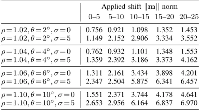
TABLE VI
SHIFT ENCODING PERFORMANCE FOR TRANSLATIONS(AVERAGE ERROR
ONLY),IN CASE SCALING AND ROTATIONS HAVE BEEN ALSO APPLIED,
CORRECTLY ESTIMATED AND INVERTED BEFORE THE COMPUTATION.
Applied shift kmk norm 0–5 5–10 10–15 15–20 20–25 ⇢ = 1.02, ✓ = 2 , = 0 0.756 0.921 1.098 1.352 1.453 ⇢ = 1.02, ✓ = 2 , = 5 1.149 2.152 2.906 3.334 3.552 ⇢ = 1.04, ✓ = 4 , = 0 0.762 0.932 1.101 1.348 1.553 ⇢ = 1.04, ✓ = 4 , = 5 1.359 2.392 3.186 3.373 4.162 ⇢ = 1.06, ✓ = 6 , = 0 1.311 2.161 3.434 3.898 4.201 ⇢ = 1.06, ✓ = 6 , = 5 2.347 2.504 5.875 6.341 6.457 ⇢ = 1.10, ✓ = 10 , = 0 1.551 2.371 3.744 4.178 4.641 ⇢ = 1.10, ✓ = 10 , = 5 2.653 2.956 6.164 6.837 6.970
the scaling factor estimation, and that the accuracy gracefully degrades as the ground-truth scaling factor increases.
Table V, instead, illustrates the case for the rotation estima-tion when the image has been shifted in [ 20, 20], again in the noiseless and noisy scenarios, averaged for all the used scaling factors. The same conclusions can be drawn for Table V as the ones for Table IV, that is shifting has no appreciable effect on the rotation estimation processing chain.
Given that the shift value estimation (done as in Fig. 6) is applied after the scaling and rotation estimation, we can expect skewed results for those cases where the scaling and/or rotation parameters have been previously incorrectly recov-ered. Table VI shows the performance of the shift estimation when the algorithm is applied to the images in the previous experiment whose scaling and rotation have been accurately estimated, that is the estimated scaling value is the closest in terms of powers of the base value to the ground truth one and the estimated rotation is within 1 of the applied one. While the experimental tests reported in Tables IV and V represent a slice of the results fixing the scaling and rotation parameters respectively, in this test the accuracy condition above is instead searched for fixing both these transformation parameters and then estimating the shift only when it is verified. Cumulatively, this condition applies for the 46% of the tested images in the noisy = 5 case. The performances are slightly inferior to those of Table I due to the limited precision for the scaling factor estimation, though the accuracy is still satisfying. B. Accuracy with respect to patch modifications
Table VII shows the results when a patch has been modified in the I image prior to the computation of h(I). Such a patch modification is not applied on J, so this experiment simulates a local detail changing in the original image. In particular, the pixels in the patch are set to the image average luminance, which of course has a strong effect on the DFT phase. This is expected to be as severe a modification as any (non-rigid) modification to an object present in the scene, as well as any object entering or leaving the image frame, could possibly be. For brevity, the test has been carried out just for translations in the image domain, thus the experiment performance should be compared to that in Table I. The modified patch is put in slightly different random positions for each database image, as
IEEE TRANSACTIONS ON INFORMATION SECURITY AND FORENSICS 10
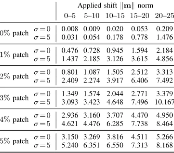
TABLE VII
SHIFT ENCODING PERFORMANCE FOR TRANSLATIONS(AVERAGE ERROR
ONLY),WHEN AN IMAGE PATCH IS MODIFIED PRIOR TO COMPUTINGh(I).
Applied shift kmk norm 0–5 5–10 10–15 15–20 20–25 0%patch = 0= 5 0.008 0.009 0.020 0.053 0.2090.031 0.054 0.178 0.778 1.476 1%patch = 0 0.476 0.728 0.945 1.594 2.184 = 5 1.437 2.185 3.126 3.615 4.856 2%patch = 0 0.801 1.087 1.505 2.512 3.313 = 5 2.409 2.274 3.917 6.406 7.492 3%patch = 0 1.349 1.574 2.044 2.771 3.379 = 5 3.093 3.423 4.648 7.496 10.167 4%patch = 0= 5 2.936 3.160 3.707 4.470 4.9504.621 4.476 6.285 7.738 8.464 5%patch = 0 3.150 3.269 3.816 4.511 5.266 = 5 5.240 6.351 6.550 7.313 8.168
well as shaped either as a square, as a rectangle or an object (in our tests, either a dog or a car), but it is always placed in the central portion of the image to avoid interference by the windowing process. The percentage of the total image area covered by the patch is varied from 1% to 5% (the latter is equivalent to a square 57⇥57 patch for the given images size). For readibility, in Table VII only average shift errors are reported, in the = 0 and = 5 cases. For the lower patch percentages the performance are only slightly degraded with respect to those shown in Table I, showing that, even if a small portion of the phase information is destroyed by changing the original image data, the algorithm is able to withstand the effects achieving a good degree of robustness. When the per-centage of the modified image increases, the recovered phase information is of course increasingly unreliable. This fragility can be indeed useful in some applications. For example, a surveillance application can easily exploit hash breaking in those contexts where slight camera movements are anticipated. C. Hash extension: modified patch localization
Following the experiments on the robustness to patch mod-ifications, in this section we propose an extension of the extracted hash to enable the localization of the modified patch. As we mentioned, the DFT phase based hash that we employed so far is a global descriptor, which is therefore unable to pinpoint any local detail missing or changed in the image I. As shown in Sec. V-B, in case where a patch has been modified there is a high probability that the rigid geometric transformation is correctly estimated nonetheless (or at least within a tolerable error margin), as long as the patch is not too large. Once the geometric transformation is found, the decoder can invert it to obtain ˆI, a good approximation of I, from the side information J. In this section we assume that is also desired to find if and where a patch in I has been modified.
Of course, many possible solutions can be found in the image matching and authentication literature to handle this problem, including robust hashing and forensics techniques that we mentioned in Sec. II. However, here we propose a
1 2 3 4 5 6 7 8 1 2 3 4 5 6 7 8 n <latexit sha1_base64="9xQZvD3cl3eq72hAv9FC784NQY8=">AAAB6HicbVBNS8NAEJ3Ur1q/qh69LBbBU0mkqMeCF48t2A9oQ9lsJ+3azSbsboQS+gu8eFDEqz/Jm//GbZuDtj4YeLw3w8y8IBFcG9f9dgobm1vbO8Xd0t7+weFR+fikreNUMWyxWMSqG1CNgktsGW4EdhOFNAoEdoLJ3dzvPKHSPJYPZpqgH9GR5CFn1FipKQflilt1FyDrxMtJBXI0BuWv/jBmaYTSMEG17nluYvyMKsOZwFmpn2pMKJvQEfYslTRC7WeLQ2fkwipDEsbKljRkof6eyGik9TQKbGdEzVivenPxP6+XmvDWz7hMUoOSLReFqSAmJvOvyZArZEZMLaFMcXsrYWOqKDM2m5INwVt9eZ20r6perVpr1ir16zyOIpzBOVyCBzdQh3toQAsYIDzDK7w5j86L8+58LFsLTj5zCn/gfP4A1buM7Q==</latexit> m
(a) Patch centered, =0.
1 2 3 4 5 6 7 8 1 2 3 4 5 6 7 8 n <latexit sha1_base64="9xQZvD3cl3eq72hAv9FC784NQY8=">AAAB6HicbVBNS8NAEJ3Ur1q/qh69LBbBU0mkqMeCF48t2A9oQ9lsJ+3azSbsboQS+gu8eFDEqz/Jm//GbZuDtj4YeLw3w8y8IBFcG9f9dgobm1vbO8Xd0t7+weFR+fikreNUMWyxWMSqG1CNgktsGW4EdhOFNAoEdoLJ3dzvPKHSPJYPZpqgH9GR5CFn1FipKQflilt1FyDrxMtJBXI0BuWv/jBmaYTSMEG17nluYvyMKsOZwFmpn2pMKJvQEfYslTRC7WeLQ2fkwipDEsbKljRkof6eyGik9TQKbGdEzVivenPxP6+XmvDWz7hMUoOSLReFqSAmJvOvyZArZEZMLaFMcXsrYWOqKDM2m5INwVt9eZ20r6perVpr1ir16zyOIpzBOVyCBzdQh3toQAsYIDzDK7w5j86L8+58LFsLTj5zCn/gfP4A1buM7Q==</latexit> m (b) Patch centered, =5. 1 2 3 4 5 6 7 8 1 2 3 4 5 6 7 8 n <latexit sha1_base64="9xQZvD3cl3eq72hAv9FC784NQY8=">AAAB6HicbVBNS8NAEJ3Ur1q/qh69LBbBU0mkqMeCF48t2A9oQ9lsJ+3azSbsboQS+gu8eFDEqz/Jm//GbZuDtj4YeLw3w8y8IBFcG9f9dgobm1vbO8Xd0t7+weFR+fikreNUMWyxWMSqG1CNgktsGW4EdhOFNAoEdoLJ3dzvPKHSPJYPZpqgH9GR5CFn1FipKQflilt1FyDrxMtJBXI0BuWv/jBmaYTSMEG17nluYvyMKsOZwFmpn2pMKJvQEfYslTRC7WeLQ2fkwipDEsbKljRkof6eyGik9TQKbGdEzVivenPxP6+XmvDWz7hMUoOSLReFqSAmJvOvyZArZEZMLaFMcXsrYWOqKDM2m5INwVt9eZ20r6perVpr1ir16zyOIpzBOVyCBzdQh3toQAsYIDzDK7w5j86L8+58LFsLTj5zCn/gfP4A1buM7Q==</latexit> m
(c) Patch not centered, =0.
1 2 3 4 5 6 7 8 1 2 3 4 5 6 7 8 n <latexit sha1_base64="9xQZvD3cl3eq72hAv9FC784NQY8=">AAAB6HicbVBNS8NAEJ3Ur1q/qh69LBbBU0mkqMeCF48t2A9oQ9lsJ+3azSbsboQS+gu8eFDEqz/Jm//GbZuDtj4YeLw3w8y8IBFcG9f9dgobm1vbO8Xd0t7+weFR+fikreNUMWyxWMSqG1CNgktsGW4EdhOFNAoEdoLJ3dzvPKHSPJYPZpqgH9GR5CFn1FipKQflilt1FyDrxMtJBXI0BuWv/jBmaYTSMEG17nluYvyMKsOZwFmpn2pMKJvQEfYslTRC7WeLQ2fkwipDEsbKljRkof6eyGik9TQKbGdEzVivenPxP6+XmvDWz7hMUoOSLReFqSAmJvOvyZArZEZMLaFMcXsrYWOqKDM2m5INwVt9eZ20r6perVpr1ir16zyOIpzBOVyCBzdQh3toQAsYIDzDK7w5j86L8+58LFsLTj5zCn/gfP4A1buM7Q==</latexit> m
(d) Patch not centered, =5.
1 2 3 4 5 6 7 8 1 2 3 4 5 6 7 8 n <latexit sha1_base64="9xQZvD3cl3eq72hAv9FC784NQY8=">AAAB6HicbVBNS8NAEJ3Ur1q/qh69LBbBU0mkqMeCF48t2A9oQ9lsJ+3azSbsboQS+gu8eFDEqz/Jm//GbZuDtj4YeLw3w8y8IBFcG9f9dgobm1vbO8Xd0t7+weFR+fikreNUMWyxWMSqG1CNgktsGW4EdhOFNAoEdoLJ3dzvPKHSPJYPZpqgH9GR5CFn1FipKQflilt1FyDrxMtJBXI0BuWv/jBmaYTSMEG17nluYvyMKsOZwFmpn2pMKJvQEfYslTRC7WeLQ2fkwipDEsbKljRkof6eyGik9TQKbGdEzVivenPxP6+XmvDWz7hMUoOSLReFqSAmJvOvyZArZEZMLaFMcXsrYWOqKDM2m5INwVt9eZ20r6perVpr1ir16zyOIpzBOVyCBzdQh3toQAsYIDzDK7w5j86L8+58LFsLTj5zCn/gfP4A1buM7Q==</latexit> m
(e) Object (car), =0.
1 2 3 4 5 6 7 8 1 2 3 4 5 6 7 8 n <latexit sha1_base64="9xQZvD3cl3eq72hAv9FC784NQY8=">AAAB6HicbVBNS8NAEJ3Ur1q/qh69LBbBU0mkqMeCF48t2A9oQ9lsJ+3azSbsboQS+gu8eFDEqz/Jm//GbZuDtj4YeLw3w8y8IBFcG9f9dgobm1vbO8Xd0t7+weFR+fikreNUMWyxWMSqG1CNgktsGW4EdhOFNAoEdoLJ3dzvPKHSPJYPZpqgH9GR5CFn1FipKQflilt1FyDrxMtJBXI0BuWv/jBmaYTSMEG17nluYvyMKsOZwFmpn2pMKJvQEfYslTRC7WeLQ2fkwipDEsbKljRkof6eyGik9TQKbGdEzVivenPxP6+XmvDWz7hMUoOSLReFqSAmJvOvyZArZEZMLaFMcXsrYWOqKDM2m5INwVt9eZ20r6perVpr1ir16zyOIpzBOVyCBzdQh3toQAsYIDzDK7w5j86L8+58LFsLTj5zCn/gfP4A1buM7Q==</latexit> m (f) Object (car), =5.
Fig. 9. Visual depiction of the average sub-hashes Hamming distance (blue is 0, green is maximum). The dotted line shows the changed patch position. For Figs. 9e–9f the silhouette of the inserted object is drawn.
solution using the same methodology employed in the rest of the paper, that is thus compatible with the computational and bandwidth constraints that we imposed on A. With respect to state-of-the-art robust hashing techniques, such as [24], [26], the proposed extension is computationally much simpler and the hash is marginally shorter, although of course those spe-cialized algorithms are explicitly targeted at image tampering and thus surely provide more flexible performance.
In the proposed solution A sends more information in addition to h(I), as follows. The central part of the image is broken into blocks. Then, each block is treated like a sub-image input to the hash extraction process and generate its own hash. The resulting matrix of sub-hashes is then sent to the decoder to be compared with that obtained from ˆI.
Here are the implementation details of this technique for the experiments at hand. The central 256⇥256 portion of the image I is divided into 32⇥32 blocks (a total of 64 blocks). Then, the sub-hashes are extracted from each block in the usual way. Let us call the matrix of sub-hashes H(n, m; I) for n, m = 1, . . . , 8, where each sub-hash H(n, m; I) is thus 4+4+4·4=24 bits long. The same procedure is applied at the decoder on ˆI, obtaining H(n, m; ˆI). The Hamming distance is computed for each (n, m) pair. The image block (or blocks) within which a patch has been modified should obtain the highest distances, thus allowing to localize the modified patch. In these experiments, a 32⇥32 square patch or an object of the same height (a dog or a car, as in Sec. V-B), is modified in the same position for every image in the dataset. In some tests the (square) patch is centered so that it is equally spread
Fig. 10. Visual examples of the non-rigid transformations applied, with no spatial shifts. The original Pentagon figure is on the left. In the middle, the image is radially distorted to simulate the distortion caused by lens curvature effects, possibly due to the small lens size. On the right, projective geometry is employed to change the view perspective, thus simulating camera tilting.
across 4 adjacent blocks, while in the others it is not. Then, the shift estimation test is performed exactly as we did for Table I. In case the shift has been recovered within a prefixed tolerance on the magnitude of the error vector (set to 2 in this case), the Hamming distance is computed for all sub-hashes. Fig. 9 shows the distances for each block averaged over all images and all tested shifts, with and without adding Gaussian noise. It clearly shows that the modified patch (or the inserted object) is accurately pinpointed. Of course, the price to pay is increased bandwidth. For these experiments, an additional 24· 64=1536 bits are sent to localize the modified patch.
Note that the just discussed matrix of sub-hashes H(n, m; I) is not a more robust version of h(I) for the global geometric transformation estimation task. Given that each sub-hash is separately obtained on relatively small blocks, they are far more susceptible to border effects when spatial shifts are performed, not to mention how hard it is to reliably track data from adjacent sub-blocks in the rotation and scaling cases. In fact, H(n, m; I) represents a good content signature only after the transformation has been more or less successfully inverted through the proposed framework involving h(I).
D. Accuracy with respect to non-rigid and photometric trans-formations
Next, let us address the proposed method performance in presence of global non-rigid and photometric transformations. Again, the experiments are limited to the spatial shift case.
Non-rigid global modifications are a challenging test for the proposed method, because differently from image registration there is no local feature matching process to help in estimating them. As we mentioned, the algorithm objective is not to estimate which non-rigid transformation occurred but rather to estimate the spatial shift despite the application of those transformations. In the scenario of Fig. 4, we have tested distortions compatible with the capturing camera at A being in slightly different conditions than those at B. Fig. 10 shows an example of the transformations that we applied in this section. The first experiments involves radial distortion on the I image (see the middle picture of Fig. 10). This is an effect typically introduced by the capturing camera lens reduced size. The results on the estimation of spatial shifting in presence of radial distortion are shown in the top part of Table VIII. The amount of introduced distortion is given in terms of the coefficients given to the first and second order terms in the
TABLE VIII
SHIFT ENCODING PERFORMANCE FOR TRANSLATIONS WHEN RADIAL
DISTORTION(TOP),PERSPECTIVE CHANGE(MIDDLE),AND PHOTOMETRIC
TRANSFORMATIONS(BOTTOM)ARE APPLIED BEFORE COMPUTINGh(I).
Applied shift kmk norm
0–5 5–10 10–15 15–20 20–25 v = [1.2, 0] Avg. error 0.094 0.113 0.311 0.493 0.596 = 0 Max. error 0.778 0.778 1.033 1.597 2.468 v = [1.2, 0] Avg. error 0.270 0.454 0.564 0.898 1.342 = 5 Max. error 0.930 1.293 2.001 2.977 3.462 v = [1.4, 0.1] Avg. error 0.107 0.102 0.211 0.532 0.802 = 0 Max. error 0.224 0.267 1.010 1.904 2.081 v = [1.4, 0.1] Avg. error 0.273 0.433 0.616 0.858 1.257 = 5 Max. error 0.392 1.352 2.076 2.869 3.069 v = [1.6, 0.2] Avg. error 0.105 0.168 0.314 0.639 0.900 = 0 Max. error 0.237 0.823 0.933 2.033 2.436 v = [1.6, 0.2] Avg. error 0.347 0.421 0.501 0.933 1.831 = 5 Max. error 0.519 1.837 1.359 3.898 5.328 l = 0.025 Avg. error 1.533 1.713 2.070 2.622 3.186 = 0 Max. error 2.360 3.090 4.358 6.246 6.323 l = 0.025 Avg. error 1.524 1.788 2.140 2.755 3.392 = 5 Max. error 2.800 3.611 4.604 6.275 6.245 l = 0.050 Avg. error 4.387 4.158 4.827 5.961 8.646 = 0 Max. error 6.593 7.634 8.731 20.99 28.89 l = 0.050 Avg. error 4.061 4.241 4.725 6.034 9.035 = 5 Max. error 6.023 7.781 8.862 19.61 27.45 l = 0.075 Avg. error 7.409 7.903 10.48 15.12 18.69 = 0 Max. error 10.52 12.50 32.54 42.15 46.17 l = 0.075 Avg. error 8.356 8.609 11.06 14.84 18.98 = 5 Max. error 10.66 12.10 33.74 40.82 43.59 Contrast Avg. error 0.002 0.003 0.017 0.024 0.066 adj., =0 Max. error 0.022 0.022 0.356 0.242 0.761 Contrast Avg. error 0.054 0.080 0.106 0.156 0.238 adj., =5 Max. error 0.228 0.250 0.768 0.973 1.201 Gaussian Avg. error 0.007 0.005 0.014 0.055 0.2418 blurring, =0 Max. error 0.022 0.031 0.712 1.422 1.898 Gaussian Avg. error 0.078 0.112 0.222 0.436 0.614 blurring, =5 Max. error 0.126 0.819 1.489 1.602 1.896
standard radial mapping formula, given in the vectors v. The distorted images have the same size of the original ones. The reported results show a remarkable amount of robustness of the spatial shift estimation with respect to radial distortions.
Moreover, we have employed projective geometry to sim-ulate a view perspective change. In particular, a significant amount of camera tilt is simulated by mapping the top cor-ners towards the inside of the image (see the right picture of Fig. 10). The results are shown in the middle part of Table VIII. The particular projective mapping, namely the amount of horizontal moving of the top left corner compared to the image side, is given by l. Thus, e.g., with l =0.075 the top side of the image is 15% narrower than the bottom side.
Since the modified image is projected on a different plane, the DFT phase has no way to distinguish between such occur-rence and a coplanar spatial shift for those pixels sufficiently far from the perspective line. We have compensated some of this effect (in our case in the vertical direction) by aligning the original and modified images center with respect to the
viewer. In fact, Table VIII shows how systematic errors are being introduced, but they are limited for a moderate amount of distortion. Otherwise the performance are pretty much com-parable with those in Table I, including the limited sensitivity to added noise. There is no difference in considering (separate) panning instead of tilting, expect that the side corners are moved instead of the top ones, and the compensation is done in the horizontal direction. Therefore, as long as camera tilting and/or panning are not expected to be too drastic, the proposed method is still able to be satisfyingly robust against perspective changes, although a little less when compared with radial distortions when considering the introduced systematic errors. Last, we have also considered photometric transformations applied on J. The results for the application of two common global photometric transformations are given in the bottom part of Table VIII, namely contrast adjustment and Gaussian blurring, both using standard parameters (stretching the his-togram in [0.1, 0.9] and applying = 5 respectively). In general, they are better tolerated by the system because the non-linear effect on the DFT phase is more moderate than in the previous cases of non-rigid transformations.
E. Comparison to local features extraction and matching In this set of experiments, we used some well-known local features in the same context as the one considered in this paper. To summarize the process, the features are extracted on I and then sent to B as the hash h(I). Then, B extracts the features on J and finally it tries to match them to the features in h(I). If rigid transformation are assumed to be applied on I to obtain J, the aim of the feature matching process is to estimate the transformation parameters.
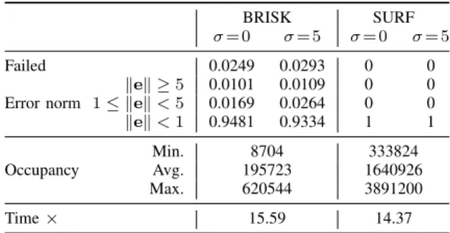
Again, just shifting in the spatial dimension is considered here for the sake of conciseness. The local features that we have tested are two among the best known local features: SURF [41] and BRISK [42]. SURF descriptors are usually given as a set of real-valued feature vectors, while BRISK descriptors are more compact since the feature vectors are constituted by unsigned integer values. The feature matching process that we employed is the one in [43].
In the left part of Table IX we reported the results obtained for the BRISK descriptors. In some cases, the feature vector is such that the feature matching process fails to produce a reliable estimation entirely, typically because it is too short. In the first row the percentage of such cases is reported. The next three rows report the error norm, which is the difference vector kek between the output shift and the ground truth shift. Such measures, with respect to the previous experiments, are given in aggregate form without separating the results depending on the ground truth shift norm since errors are rarer. Cumulatively, the BRISK descriptors fail to give an accurate estimation of the shift (kek < 1) in just above the 5% of the tests in both the noiseless and noisy case. The next rows report the the minimum, maximum and average occupancy of the feature vectors in bits for the given dataset (we have not considered any other necessary information on the extracted feature points). The average feature vector is roughly 2500 times longer than the 80 bits employed in this work. The last
TABLE IX
RESULTS USING THEBRISKANDSURFLOCAL DESCRIPTORS.
BRISK SURF
= 0 = 5 = 0 = 5
Failed 0.0249 0.0293 0 0
Error norm 1 kek < 5kek 5 0.01010.0169 0.01090.0264 00 00 kek < 1 0.9481 0.9334 1 1 Occupancy Min.Avg. 1957238704 1640926333824
Max. 620544 3891200
Time ⇥ 15.59 14.37
row gives the average time increase for the extraction process, thus excluding the complex feature matching procedure. For the BRISK descriptors, the extraction is approximately 15 times slower than the FFT phase sign extraction, which on the average takes 3.46ms on a sub-standard desktop computer.
The right part of Table IX concerns the SURF descriptors. In the experiments that we have run, the output shift has always been accurate without fail. On the other hand, the transmitted hash data rate is at least another order of magnitude greater than that of the BRISK descriptors, on the average being approximately 20000 times higher. In addition, the run time is still 14 times greater than the proposed method.
In conclusion, these results show nicely the tradeoff between geometric transformation estimation accuracy, computational complexity and hash data rate in the discussed problem. It is clear that the more voluminous the sent data is, the more accurate the estimation becomes, and the proposed algorithm sits at the far end on the data rate scale. The comparison shown here proves the point that, since it targets only rigid geometric transformation, the proposed method trades an acceptable de-cline in accuracy with respect to local feature based matching algorithms in return for using very few bits for the hash and negligible computational power for its extraction. There can also be some drawbacks in terms of security when employing local descriptors: this is discussed in the next subsection. F. Security
The following brief discussion is focused on the security of the hashing technique at the application layer, that is assuming that the lower levels of the communication infrastructure are effectively shielding the system from the kind of attacks en-compassing them. For example, jamming the communication between the sensor devices (A) and the central entity (B) may be a possible security concern in an application scenario where the timely relaying of h(I) is critical, and in that case it needs to be addressed at the link layer using anti-jamming codes and protocols. Instead, security as intended in Fig. 4 refers to the amount and quality of information on the image I knowable by an eavesdropper C from its condensed version h(I).
Of course, the critical assumption still is the physical inaccessibility of either A or B. The only security threat to consider for C is eavesdropping because any other tampering process needs first to know a legitimate h(I). In other words, there is no other reason for the attacker to inject a fraudulent