Universit`
a degli Studi di Ferrara
FACOLT `A DI SCIENZE MATEMATICHE FISICHE E NATURALI
Dottorato di Ricerca in Fisica Ciclo XXI
Dalitz Plot Study
of the Charmless Decay
B
+
→ K
S
π
+
π
0
with the B
A
B
AR
Detector
Dottorando:
Dott. Paolo Franchini
Tutore: Prof. Roberto Calabrese
Correlatore: Dott. Concezio Bozzi
Contents
Introduction v
1 Theory Overview 1
1.1 CP violation . . . 1
1.1.1 CP symmetry in quantum mechanics . . . 1
1.1.2 CP violation in the Standard Model. . . 9
1.2 The B+ → K Sπ+π0 decay . . . 11
1.2.1 Experimental and theoretical status . . . 11
1.2.2 Constraints on γ angle from B → Kππ modes . . . 14
1.3 Three-body decays . . . 17
1.3.1 Introduction . . . 17
1.3.2 Kinematics of the three-body decays . . . 18
1.3.3 The isobar model . . . 20
1.3.4 Mass term description . . . 22
1.3.5 Barrier factors. . . 23
1.3.6 Angular dependence and helicity angles . . . 25
1.3.7 Square Dalitz plot . . . 26
2 The BABAR Experiment 29 2.1 The PEP-II Asymmetric Collider . . . 30
2.1.1 PEP-II Backgrounds . . . 33
2.2 The BABAR Detector . . . 34
2.2.1 Silicon Vertex Tracker (SVT) . . . 36
2.2.2 Drift Chamber (DCH) . . . 37
2.2.3 Cerenkov Light Detector (Dˇ RC) . . . 40
2.2.4 Electromagnetic Calorimeter (EMC) . . . 43
2.2.5 Instrumented Flux Return (IFR) . . . 45
2.2.6 Trigger System (TRG) and Data Acquisition (DAQ) . . . 53
3 The analysis method 55 3.1 Monte Carlo . . . 55 3.2 Reconstruction . . . 57 3.2.1 Tracking algorithms. . . 57 3.2.2 Calorimeter algorithms . . . 59 3.2.3 Particle identification . . . 59 3.2.4 Vertexing of candidates. . . 60 3.3 Discriminating variables . . . 61 3.3.1 Kinematic variables . . . 61 3.3.2 Event-shape variables. . . 63 3.3.3 Neural network . . . 67
3.4 Maximum Likelihood Fits . . . 69
3.4.1 Extended Maximum Likelihood Fits. . . 70
3.4.2 Error estimation . . . 71
3.4.3 Toy Monte Carlo . . . 71
3.4.4 Extraction of physical parameters . . . 72
4 The analysis 73 4.1 Overview. . . 73
4.2 Dependence of the discriminating variables on the DP . . . 75
4.3 Event selection . . . 75
4.3.1 Multiple candidates . . . 78
4.4 Treatment of Self Cross Feed . . . 81
4.6 B ¯B background . . . 88
4.6.1 Determination of B background modes . . . 88
4.7 Control sample . . . 93
4.7.1 D¯0 shape in the Dalitz plot . . . . 96
4.7.2 B+ → ¯D0(→ K0 Sπ0)π+ used as control sample . . . 98
4.8 The total likelihood . . . 98
4.8.1 The likelihood function . . . 101
4.8.2 Correlations among observables . . . 103
4.8.3 The Dalitz plot PDFs . . . 105
4.8.4 The other PDFs. . . 109
4.8.5 The fit parameters . . . 113
5 Results 117 5.1 Decay model . . . 117
5.2 Pure toys MC tests . . . 118
5.2.1 High statistics signal-only toys . . . 118
5.3 Toys and embedded fits with realistic yields . . . 120
5.3.1 D0 and fit stability . . . . 124
5.4 Test of the fit on fully simulated MC tests . . . 127
5.4.1 Freezing the nominal fit . . . 127
5.4.2 Fit results . . . 128
5.4.3 Likelihood ratios . . . 132
5.4.4 Discriminant variables projection plots . . . 132
5.4.5 Dalitz plot projection plots. . . 132
5.5 Results on data . . . 135
5.5.1 Fit result . . . 135
5.5.2 CP blind fit . . . 136
5.5.3 Fit allowing for CP violation (nominal fit) . . . 136
6 Systematics 151
6.1 Detector related effects . . . 152
6.1.1 Charged particle tracking . . . 152
6.1.2 KS reconstruction . . . 152
6.1.3 Reconstruction of neutral particles . . . 153
6.2 Extra Resonances in the signal model . . . 154
6.3 Shape parameters . . . 154
6.4 B-background . . . 154
6.5 Lineshapes . . . 154
6.6 Continuum Dalitz plot PDF . . . 155
6.7 Fit Bias . . . 155
6.8 Systematics Summary . . . 155
6.9 Branching ratio uncertainties . . . 155
7 Conclusions 157 7.1 Conclusions . . . 157
A Appendix 159 A.1 Toy studies . . . 159
A.2 Systematics . . . 170
Introduction
This thesis presents preliminary measurements of decays of B mesons in charmless final states, by using a data sample of 365 millions of B ¯B pairs collected by the BABAR detector
at the PEP-II Asymmetric B Factory, located at the Stanford Linear Accelerator Center. Recently many three-body B decay modes have been observed with branching ra-tios of order 10−5. As an example ¯B0 → K
SKSKS ((6.9 ± 0.8) × 10−6), B0 → K+π−π0 ((34.9 ± 2.1) × 10−6), B0 → K0π+π− ((43.0 ± 2.3) × 10−6) and B− → π+π−π−
((16.2 ± 1.2) × 10−6).
The three-body meson decays are more complicated than two-body decays as they receive resonant and non-resonant contributions. They are generally dominated by inter-mediate vector and scalar resonances, namely, they proceed via quasi-two-body decays containing a resonance state and a pseudoscalar meson. Indeed, most of the quasi-two-body B decays are extracted from the analysis of three-quasi-two-body B decays using the Dalitz plot technique, in order to study the properties of various resonances. The non-resonant contribution is usually believed to be a small fraction of the total three-body decay rate. The study of charmless hadronic B decays can make important contributions to the understanding of models of hadronic decays.
The Dalitz plot analysis of three-body B decays provides a nice methodology for ex-tracting information on the unitary triangle in the standard model and can help the understanding of CP violation. Studies of charmless three-body decays in B → Kππ system combined with theoretical assumption, allow to put constraints on γ angle of the Cabibbo-Kobayashi-Maskawa matrix.
This is the first study of the charmless decay of the charged B meson into three-body
final state K0
S π+ π0.
This thesis is organized as follows. The theory of the three-body charmless decays is reviewed in Chapter1, together with a brief reminder of CP violation. Chapter2presents an overview of the BABAR detector used to collect the data studied in the analysis. The experimental techniques used to reconstruct events and identify particles are presented in Chapter 3. The studies performed on the Monte Carlo in order to discriminate the signal from the backgrounds are collected in Chapter4. In Chapter 5the steps done to validate the fitter are discussed, and the final fit on the data is presented. Chapter 6presents the evaluation of systematic uncertainties. In Chapter 7 we show the results for branching ratios and CP asymmetries for the three-body decay under study.
The results presented in this thesis are preliminary and show the potential capabil-ities that can be obtained with the BABAR dataset. The current measurements exhibit a discrepancy between some fit results and the actual data, which is possibly due to backgrounds being not correctly estimated and/or parametrized. Further studies are under way in order to understand these discrepancies and solve them. The results shown in these thesis have not been internally reviewed by the BABAR collaboration; therefore,
Chapter 1
Theory Overview
1.1
CP violation
1.1.1 CP symmetry in quantum mechanics
Discrete symmetries
Classical physics is invariant for symmetries of left-right inversion (parity) and for reversal of the time.
The symmetry under parity corresponds to the physical invariance of two coordinate systems with opposite sign of the space coordinates (like two rotated systems, looking each other in a mirror). A right-handed system under parity becomes left-handed. Thus the parity transformation has the same effects of a mirror reflection, and can be demonstrated that all the physics equation are invariant under this kind of transformation.
The time reversal consists of changing the sign of the time coordinate t.
For each symmetry there is a transformation, that can be associated to an operator (in this case P and T ). If an operator working on a function, has for result the same function with just an overall phase, this means that the function is invariant under that transformation, therefore the function owns a symmetry.
The symmetry under transformation of charge conjugation is not present in classical physics, represented by the operator C. This symmetry, where exists, means that a so-called “antiparticle” with the opposite charge is present for each particle; this result can be assumed only in relativistic quantum mechanics, where to each particle field, can be associated a field with opposite charge quantum number: the antiparticle.
In particle physics, described by the Standard Model, the electromagnetic and strong interactions preserve P, C and T, one by one, while the weak interactions violate P and C separately. However, the composite transformation CPT is a symmetry preserved in all the universe, that means in each lagrangian field theory experimentally tested.
The parity violation in weak interactions was suggested for the first time in 1956 by Lee and Yang [2], before the experimental evidences coming from studies of pseudoscalar quantities (first of all the particle helicity). Historical experiments of great importance in testing the weak intaction were done by Garwin et al. and Wu et al. in 1957 [4], Goldhaber et al. in 1958 [5] who measured the neutrino helicity.
In weak interactions C and P are both violated at the same time, so at the end the symmetry under CP was considered preserved.
A first clear evidence of CP violation comes in 1964 [6] in the K0
L decay, who was seen
to be not symmetric in the two C-conjugated decay modes, as was expected consider-ing the neutral K0
L the antiparticle of itself. Therefore the KL0 is not eigenstate of CP
transformation.
CP violation has a great theoretical importance:
• the barionic asymmetry (there is much more matter than antimatter in the observed universe), could only be generated from an initial situation in which the amount of matter and antimatter were equal, balance that has evolved after CP violating processed [7];
• elementary particles can have an electric dipole moment, who violates both P and T symmetries. In the case of T violation, CPT has to be conserved, so a CP violation is necessary at the end of the game.
In quantum mechanics the transformations P, T and C, are associated to operators
P, T and C respectively. Operators like T are written by exponentiation of
transforma-tion generators. A different approach should be used for P and C operators, who don’t correspond to continuous transformations, since are transformation associated to finite quantum numbers. P and C operators can by defined only by not taking into account the weak interaction, since it is necessary to commute with the hamiltonian operator H,
that generate the time translactions; operators can commute only when their relative transformations correspond to symmetries not violated in the theory described by the hamiltonian. Both P and C symmetries are not good symmetries of Nature, their oper-ators can be defined only switching off the weak interaction, since they do not commute with the hamiltonian of the weak interaction.
P and C are unitary. They correspond to discrete transformations, therefore they can
be associated to their eigenstates, that means multiplicative quantum numbers (at the opposite side, for the continuum transformation, quantum numbers are additive).
T is antiunitary. T can have two different eigenvalues, therefore it cannot be associated
to any quantum number. To be very precise is not correct to say that T is conserved (nothing is conserved), but is just valid the invariance under T.
We can improperly say that CPT is conserved (“CPT theorem” that is kind of preju-dice). CPT conservation means that a CP violation has to be connected to a T violation. The violations or conservations of some symmetries are related to the theory (the hamil-tonian) and not to the single observables.
Strong and weak phases
The presence of complex phases in the transition amplitude is closely related to the CP violation. Only the phases that are rephasing-invariant may have a physical meaning, and in particular lead to CP violation. Those phases are in general the relative phases of the various coherent contributions to a particular transition amplitude.
Three kind of phases may arise in transition amplitudes:
• weak or odd phase: is defined to be one which has opposite signs in the transition
amplitude for a process and in the transition amplitude for its CP-conjugate process;
• strong or even phase: has the same sign in the transition amplitude for its
CP-conjugate process;
• spurious phase: is a conventional relative phase between the amplitude and the
Given CP conjugated states i and ¯i, f and ¯f , g and ¯g, where for example
CP|f i = eiξf| ¯f i (1.1)
with arbitrary phase ξf considered equal to 1, CP violation is possible when the transition
amplitudes are the sum of two or more transition amplitudes with different strong or weak phases, like
hf |T |ii = A1ei(δ1+φ1)+ A2ei(δ2+φ2) (1.2)
where the CP-conjugate amplitude is
h ¯f |T |¯ii = A1ei(δ1−φ1+θ)+ A2ei(δ2−φ2+θ) (1.3)
where T is the transition matrix, A1 and A2 the modules of the transition amplitudes,
and δ1 6= δ2 (CP strong phases), φ1 6= φ2 (CP weak phases) and θ the common spurious
phase. The asymmetry between the two amplitudes is
|hf |T |ii|2− |h ¯f |T |¯ii|2
|hf |T |ii|2+ |h ¯f |T |¯ii|2 (1.4)
It is possible to have CP violation even in absence of strong phases or amplitudes interference, for quantities like this
hf |T |iihg|T |¯ii − nfnghg|T |iihf |T |¯ii = 2iA1A2ei(δ1+δ2+θ)sin(φ1− φ2) (1.5)
where there is a relationship between the two final states f and g, like for physical states that are a superposition of two CP eigenstates.
In any case, due to CPT invariance, the total decay width of i and ¯i has to be equal X
f
|hf |T |ii|2 =X
f
|h ¯f |T |¯ii|2 (1.6)
therefore it is necessary to study CP violation using partial decay channels of the particles, since it is precluded the observation of CP-violating difference between the total decay width of a particle and its antiparticle.
Neutral meson system
The neutral mesons, interesting for the study of CP violation, decay mostly through weak interactions. Let’s consider a generic neutral meson (that can be the a D0, K0, B0
d or Bs0) P0 with antiparticle ¯P0, and common mass m
• |P0i and | ¯P0i are eigenstates of strong and electromagnetic interactions with mass m0, so they are flavor eigenstates1;
• as consequence of the weak interaction, described by the non vanishing HW, the two
states oscillate between themselves before decaying.
At a certain time t it is possible to have a state that is a superposition of initial states and final states |nii, where the two |P0i and | ¯P0i may decay
a(t)|P0i + b(t)| ¯P0i +X
n
ci(t)|nii (1.7)
where ci(t = 0) = 0 are the amplitudes of the final states.
In the Wigner-Weisskopf [8] approximation, taking into account the interaction HW
|ψ(t)i ' ψ1(t)|P0i + ψ2(t)| ¯P0i (1.8)
where the wave function satisfies an equation equivalent to the Schr¨odinger equation
id dt µ ψ1 ψ2 ¶ = µ R11 R12 R21 R22 ¶ µ ψ1 ψ2 ¶ (1.9) where R = M − i 2Γ (1.10) with M = 1 2(R + R†), Γ = i(R − R†) (1.11)
The matrices M e Γ are hermitian, while the matrix R is anti-hermitian. The weak interaction is considered like a small perturbation with respect to the strong and electro-magnetic interactions; in second-order perturbation theory the matrices M e Γ, by sums over intermediate states n, are
Mij = m0δij+ hi|HW|ji +
X
n
Phi|HW|nihn|HW|ji m0 − En
, (1.12)
Γij = 2πX
n
δ(m0− En)hi|HW|nihn|HW|ji (1.13)
where the operator P projects out the principal part and En are the energies of the states.
From the second order expansion the box Feynman diagrams came out. The mass matrix has first and second order terms, therefore virtual states connect the real states.
It follows that d dt(|ψ1| 2+ |ψ 2|2) = −(ψ∗1ψ∗1)Γ µ ψ1 ψ2 ¶ (1.14) where the left-hand side of the equation (1.14) must be negative (since the mesons decay), hence the Γ is positive definite.
The eigenstates of R are complex, since the matrix is not-hermitian, so they can be defined as µH = mH − 2iΓH, µL= mL− 2iΓL (1.15) Then we define ∆m = mH − mL > 0, ∆Γ = ΓH − ΓL, ∆µ = µH − µL (1.16)
from which we can obtain
∆m = 2|M12| (1.17)
These eigenstates and eigenvectors correspond to particles with different masses m and timelifes (or decay width) Γ; hence is possible to label them taking into account one of that two characteristics: in this case they are labelled with H and L, for the heavy and for the light respectively, having in mind the mass differences. This decision is suitable for the B0 − ¯B0 system, where the two mass eigenstates have a relevant mass difference
with respect to the lifetimes difference. For the system K0− ¯K0, is better to take into
account the lifetimes, being the filetime of one particle really longer in comparison with the other one (using thus labels L and S for the long-lived and short-lived respectively).
As already considered, under a CP transformation
CP|P0i = eiξ| ¯P0i,
CP| ¯P0i = e−iξ|P0i (1.18)
with arbitrary phase ξ. Hence is possible to define the two CP eigenstates as
|P±i =
1
√
2(|P
We have a CP invariance for a theory described by an hamiltonian for the weak inter-action HW, if
(CP)HW(CP)† = HW (1.20)
which implies that Γ11= Γ22 and analogously M11= M22. Since M21= e2iξM12,
Γ21 = e2iξΓ12 (1.21)
we get |R11| = |R22|.
It is convenient to introduce the CP-violating parameters
δ = |R12| − |R21| |R12| + |R21| , θ = R22− R11 ∆µ (1.22)
The eigenstates R, that are the mass eigenvectors (eigenvectors of the weak interac-tion), can be defined as follows
|PHi = pH|P0i + qH| ¯P0i,
|PLi = pL|P0i − qL| ¯P0i (1.23)
Unlike |P0i and | ¯P0i, the mass eigenstates evolve as a function of time, according to
the equation (1.9).
|PH(t)i = e−iµHt|PHi,
|PL(t)i = e−iµLt|PLi. (1.24)
Due to the weak interaction, described by HW, these states evolve like an exponential
function with defined masses mH and mL, and defined decay width ΓH and ΓL, according
to eq. (1.15). The probability to observe P0 or ¯P0 is proportional to e−Γt. Starting with
a flavor eigenstate like P0 (that can be written in terms of mass eigenstates) produced by
the strong interaction, it evolves during the time, displaying the possibility to observe a flavor eigenstate of the second kind like ¯P0.
The phase between |PHi and |PLi is not defined, and it is present in the product hPH|PLi, which gives
|hPH|PLi|2 =
(1 + δ2)|1 − θ2| − (1 − δ2)(1 − |θ|2)
(1 + δ2)|1 − θ2| + (1 − δ2)(1 + |θ|2) (1.25)
therefore from CP invariance, that oblige to have the parameters δ = θ = 0, it follows that
hPH|PLi = 0. Imposing a convention for the phases of |PHi and |PLi like for eq. (1.23),
Since CP violation is small, assuming that CPT conserved (so qH/pH = qL/pL = q/p)
gives
|PHi = (1 + ²)|P0i + (1 − ²)| ¯P0i ' |P+i,
|PLi = (1 + ²)|P0i − (1 − ²)| ¯P0i ' |P−i (1.26)
where the parameter
² = p − q
p + q (1.27)
allows to quantify the CP violation. In presence of CP violation the mass eigenstates are not orthogonal, and are not equal to the CP eigenstates.
Classification of CP violation If CP is conserved M∗ 12= e2iξM12, Γ∗ 12= e2iξΓ12, q p = ±e iξ (1.28)
and the CP eigenstates are equal to the mass eigenstates
CP|PHi = ±|PHi,
CP|PLi = ∓|PLi (1.29)
where the sign ambiguity can be solved only by experiments. The condition to have CP
invariance is ¯ ¯ ¯ ¯qp ¯ ¯ ¯ ¯ = 1 (1.30)
The CP transformation acts on a final state f in this straightforward way
CP|f i = eiξf| ¯f i,
CP| ¯f i = e−iξf|f i (1.31)
so for the decay amplitudes, taking into account equation (1.18), we have ¯
Af = ei(ξf−ξ)Af,
Af¯= ei(ξf+ξ)A¯f (1.32)
hence, avoiding the arbitrary phases ξ and ξf, to have CP invariance we need to satisfy
the conditions
|Af| = | ¯Af¯|,
|Af¯| = | ¯Af| (1.33)
At the end from equations1.28 and 1.32 follows that arg µ p2 q2AfA¯ ∗ fAf¯A¯∗f¯ ¶ = 0 (1.34)
There are tree species of CP violation:
• indirect CP violation: CP violation in the mixing between the flavor eigenstates,
when 1.30 does not hold;
• direct CP violation: CP violation in the decay amplitudes, when 1.33 does not hold;
• interference CP violation: CP violation in the phase mismatch between the mixing
parameters (p, q) and the decay amplitudes, when 1.34 does not hold.
To summarize, CP violation arises always from an interference between phases, phases of the elements M12 and Γ12 (indirect), phases of two decay amplitudes (direct), or phase of p/q and the phases of the decay amplitudes (interference).
1.1.2 CP violation in the Standard Model
The charged current term of the electro-weak lagrangian (mediated by the W± boson),
written for the mass eigenstates of just one quark family, is
LqW = √g
2(W
+
µu¯LγµV dL+ Wµ−d¯LγµV†uL) (1.35)
where V is an element of the Cabibbo-Kobayashi-Maskawa (CKM) matrix [11] [12]. For three quark families
V = VVudcd VVuscs VVubcb Vtd Vts Vtb (1.36)
It is a unitary matrix2, with 4 independent parameters and one phase that, as observed
for the first time by Kobayashi and Maskawa, generates CP violation [12]. There is not an analog matrix for the neutral currents, since flavor changing neutral currents do not exists at the tree level.
There is CP violation in the Standard Model, if, and only if, any of the rephasing-invariant functions of the CKM matrix is not real.
Unitarity Triangle
Taking into account the unitarity conditions of the CKM matrix, the following relations hold
VudVus∗ + VcdVcs∗ + VtdVts∗ = 0, VusVub∗ + VcsVcb∗+ VtsVtb∗ = 0, VudVub∗ + VcdVcb∗ + VtdVtb∗ = 0.
(1.37)
these are sums of three complex quantities, that can be represented in the complex plane as sides of a triangle; the lenghts of the sides are invariant, so the triangle does not modify its shape under a rephasing of all the phases.
From experimental measurements of Vij, the triangles coming out from the first two
equations of 1.37 have a side much shorter than other two, these triangles are connected to CP violation in the K and Bs system respectively.
The most interesting triangle, related with the physics of the Bd meson, is the third
one built from the orthogonality condition between the first and the second columns of the matrix. It is the so called “Unitarity Triangle”[13].
Choosing a convention for the phases and rescaling the triangle by dividing each side by |VcdVcb∗|, we obtain the triangle of Figure 1.1. The inner angles of the triangle are
α = arg µ −VtdV ∗ tb VudVub∗ ¶ , β = arg µ −VcdVcb∗ VtdVtb∗ ¶ , γ = arg µ −VudV ∗ cb VcdVcb∗ ¶ . (1.38) Wolfenstein parametrization
The first parametrization of the CKM matrix was put forward by Kobayashi and Maskawa using the three Euler angles, writing the matrix like a product of three rotations.
In 1983 it was realized that the bottom quark b decays predominantly to the charm quark c, so |Vcb| À |Vub|; then it was noticed by Wolfenstein that |Vcb| ∼ |Vus2|, and [14] a
parametrization in which unitarity only holds approximately was introduced, writing
V =
1 − λ
2/2 λ Aλ3(ρ − iη)
−λ 1 − λ2/2 Aλ2
Aλ3(1 − ρ − iη) −Aλ2 1
+ O(λ4) (1.39)
involving the parameters λ, A, ρ and η, where λ = sin θC ' 0.22 is small and serves as
an expansion parameter, that is a function of the Cabibbo angle θC, A ' 0.82 and η
rapresent the CP violation phase. We have CP violation if η 6= 0, that means a triangle area not equal to zero.
In the Wolfenstein parametrization the CKM matrix elements satisfy these relations
VudVub∗ |VcdVcb| = ρ + iη, VcdVcb∗ |VcdVcb| = −1, VtdVtb∗ |VcdVcb| = 1 − ρ − iη. (1.40)
1.2
The B
+→ K
Sπ
+π
0decay
1.2.1 Experimental and theoretical status
The B+ → K
Sπ+π0 decay3 proceeds via quasi-2-body channels, B+ → K∗+π0, B+ → K∗0π+ and B+→ ρ+K0
S, or via the non resonant 3-body decay. The K∗ and ρ resonances decay into Kπ and ππ final states respectively. Many resonances overlap in
b u + B + W u u s u *+ K 0 π b u + B + W s u g u u 0 π *+ K b u + B + W u u s u *+ K 0 π b u + B + W s u g u u 0 π *+ K
Figure 1.2: Trees (left column) and penguins (right column) Feynman diagrams, where the first row are the colour suppressed and the second row the colour favoured diagrams.
Mode PDG avg. [40] BABAR ref. Belle ref. CLEO ref. New avg.
K∗(892)0π+ 10.9 ± 1.8 10.8 ± 0.6+1.1 −1.3 [15] 9.7 ± 0.6+0.8−0.9 [16] 7.6+3.5−3.0 ± 1.6 [17] 10.0 ± 0.8 K∗(892)+π0 6.9 ± 2.4 6.9 ± 2.0 ± 1.3 [18] 7.1+11.4 −7.1 ± 1.0 [17] 6.9 ± 2.3 K∗ 0(1430)0π+ 47 ± 5 32.0 ± 1.2+10.8−6.0 [15] 51.6 ± 1.7+7.0−7.4 [16] 45.2+6.2−6.3 K∗ 2(1430)0π+ < 6.9 5.6 ± 1.2+1.8−0.8 [15] < 6.9 [19] 5.6+2.2−1.4 K∗(1410)0π+ < 45 < 45 [19] < 45 K∗ 0(1680)0π+ < 12 < 15 [20] < 12 [19] < 12 K0π+π0(N.R.) < 66 < 66 [21] < 66 K0 Sρ+ 8.0 ± 1.5 8.0+1.4−1.3± 0.6 [22] < 48 [23] 8.0 +1.5 −1.4
Table 1.1: Compilation of the B0 → K0
Sπ
+π0 results. Snapshot of December 2008. B+ Branching
Fractions (decays with kaons) (×106). (UL 90% CL).
phase space, therefore is required an amplitude (Dalitz plot) analysis of the 3-body final states (see section1.3). Measurements existing up to now are included in table1.1. While all final states can be reached via colour allowed penguin diagram and annihilation dia-grams, the B+ → K∗+π0 can also proceed through color allowed and color suppressed tree
and penguin graphs (Figure 1.2) with CKM factors λ4 and λ2 respectively. The gluonic
penguin processes are favored by color and CKM. The electroweak penguin transitions might be sizeable as well.
The most important decays channel that contribute to the final 3-body state are listed in table 1.2.1 together with the branching fraction prediction; table 1.1 shows the corre-spondingly measured branching fractions.
Mode Model ref. B.F. prediction ρ(770)±K0 QCDF [24] 10.27±1.96 global fit [25] 6.08±0.79 HMChPT [26] 1.3 +3.0 −0.9 K∗(892)±π0 QCDF [24] 5.25±0.83 global fit [25] 7.00±4.49 HMChPT [26] 1.5+0.3 −0.3 FSI [27] 12.4+1.5 −0.8 K∗(892)0π± QCDF [24] 8.90±1.59 global fit [25] 10.64±0.82 HMChPT [26] 1.5+0.4 −0.3 FSI [27] 22.5+2.8−0.9 K∗(1430)±π0 HMChPT [26] 5.5+1.6 −1.4 K∗(1430)0π± HMChPT [26] 5.2+1.6 −1.4 K0π±π0 HMChPT [26] 10.0+7.1 −3.7
Table 1.2: Theoretical predictions (×106) for various models of the signal model of the Dalitz analysis,
together with a global fit. The models listed are: QCD factorization (QCDF), heavy meson chiral perturbation theory (HMChPT) and final-state interaction (FSI).
the factorization approach [26], the decay amplitude consists of three distinct factorizable terms: the current-induced process, the transition process and the annihilation process.
Recently, Belle has measured the direct CP violations B− → Kπ decay [28] that for
the charge B is
ACP(B− → K−π0) =
Γ(B− → K−π0) − Γ(B+ → K+π0)
Γ(B− → K−π0) + Γ(B+ → K+π0) = +0.07 ± 0.03 ± 0.01, (1.41)
and the average of the current experimental data of BABAR , Belle, CLEO and CDF by the Heavy Flavor Averanging Group (HFAG) [29] is
ACP(B− → K−π0) = 0.050 ± 0.025 (1.42)
A difference is observed between direct CP violations in charged and neutral modes, that by the HFAG average is
∆A = ACP(B− → K−π0) − ACP( ¯B0 → K−π+) = 0.147 ± 0.028 (1.43)
at 5σ level; however, recent calculations based on the QCD factorization approach (QCDF), the perturbative QCD approach (pQCD) and the soft-collinear effective theory
(SCET), predicted that ACP(B−→ K−π0) and ACP( ¯B0 → K−π+) are close to each other.
The mismatch between theory and experiment is maybe due to the limited understanding of the strong dynamics in B decays, but equally possibly due to new physics effects.
Even recent theoretical estimations within the QCDF framework give ACP(B− → K−π0) = −0.109 ± 0.008 [24], very close to A
CP( ¯B0 → K−π+), but still in sharp contrast
to experimental data. So it is very hard to accommodate the measured large difference ∆A in the SM with the available approaches for hadron-dynamics in B decays, even varying the value of the effective gluon mass that enter in the models. This could be an indication of new sources of CP violation beyond the SM. Using a set of FCNC effective NP operators (b → su¯u and b → sd ¯d) the results are more consistent with the experimental data for ACP(B−→ K−π0).
1.2.2 Constraints on γ angle from B → Kππ modes
The current methods to measure γ rely on the interference between the colour-allowed
B− → D0K− and the colour-suppressed B− → ¯D0K− decay modes resulting in direct CP violation. They are theoretically very clean, as only tree amplitudes are involved,
but their sensitivity to γ is governed by the rather small relative magnitude of the two amplitudes, denoted rB: 0.05 . rB . 0.3, depending on the D meson decay channel. As
a consequence, γ is the most poorly determined angle of the unitarity triangle, (78 ± 12)◦
using only direct determinations (c.f. β = (22.0 ± 0.8)◦ with the full fit) [30]. Therefore,
any independent determinations of the angle γ should be exploited in order to reduce the statistical uncertainty. Although a first proposal on using the charmless three-body decays
B → Kππ to extract the unitarity triangle angle γ via isospin relations was made in 2002
[31], the more recent ideas in [32] [33] are both far more accurate in their estimations of the theoretical uncertainties of their methods, and more convenient experimentally.
The paper by Ciuchini, Pierini and Silvestrini [33] exploits the use of the phase-extraction capabilities of the Dalitz plot analysis technique, similarly to what Lipkin-Nir-Quinn-Synder proposed to measure α in B0 → ρπ → π+π−π0 [34]. They start by
relating the ratio of the amplitudes for the decays B+ → K∗+π0 and B+ → K∗0π+ and
plot to determine the phase difference between the two B flavours.
Isospin ensures that amplitudes with the same topology are approximately equal for the two modes. Neglecting for simplicity the electro-weak penguin contribution, it is possible to write the amplitudes using isospin symmetry, in terms of Renormalization Group Invariant complex parameters, and obtain for our channel (factorizing out their CKM elements and grouping them accordingly):
√
2A(K∗+π0) = V∗
tbVtsP1− Vub∗Vus(E1+ E2+ A1− P1GIM), (1.44) A(K∗0π+) = −V∗
tbVtsP1+ Vub∗Vus(A1− P1GIM), (1.45)
where unitary triangle relations have been used to separate the penguin amplitude into CKM-favoured (P1) and CKM-suppressed (P1GIM) contributions; A1 is the disconnected
annihilation and E1(E2) the connected (disconnected) emission topologies. Recalling that
the amplitude for the C-conjugate B− process is obtained simply by complex-conjugating
the CKM factors, we can use the previous isospin relations to cancel out the penguin terms: A+ = A(K∗0π+) +√2A(K∗+π0) (1.46) = −V∗ ubVus(E1+ E2), (1.47) A− = A( ¯K∗0π−) +√2A(K∗−π0) (1.48) = −VubVus∗(E1+ E2), (1.49) whose ratio is R∓ = A − A+ = VubVus∗ V∗ ubVus = e−2iγ (1.50)
that provides a clean determination of the weak phase γ.
A±can be extracted from the 3-body decay chains B± → K∗±(→ K
Sπ±)π0 and B± → K∗0(→ K0π0)π± entering the K
Sπ±π0 Dalitz plot. Electric charge forbids the extraction
of the relative phase of the two Dalitz plots amplitudes A(K∗±π0) and A(K∗0π±) in a
straightforward way. One possibility is to use the penguin-dominated channel K∗0π+ to
fix the phase difference between the amplitudes in the two Dalitz plots. In this way an independent, albeit more uncertain, determination of γ can be obtained from R∓. In any
case the determination of γ is not as theoretically clean as the one obtained from the neutral B decays, using similar isospin relations that bring to a ratio
R0 = A¯0 A0 = VubVus∗ V∗ ubVus = e−2iγ (1.51) where A0 = A(K∗+π−) +√2A(K∗0π0) (1.52) ¯ A0 = A(K∗−π+) +√2A( ¯K∗0π0). (1.53)
In the above discussion, the so-called electroweak penguins (obtained by exchanging the gluon in the penguin diagrams by a photon) have been ignored. These result in isospin-breaking effects due, among other things, to the different electric charges of the u and d quarks, and precision measurements must take these into account. By considering the full (weak, strong and electromagnetic) effective Hamiltonian for the transition, the authors of [11] give the following final expression:
R∓= e−i(2γ+arg(1+kEW))× (1 + ∆) (1.54)
where ∆ is the theoretically bound (. 0.05) and kEW is
kEW = 3 2 CEW + C+ µ 1 + 1 − λ 2 λ2(¯ρ − i¯η) + O(λ2) ¶ (1.55) with CEW
+ and C+ being, respectively, the coefficients of the electroweak and normal QCD
4-quark operators in the effective theory. The experimental results for both R0 and R∓
can be translated into allowed regions in the ¯ρ − ¯η plane.
That model was tested using the B0 → K+π−π+ and B0 → K
Sπ+π− decays to fix
the relative phase of neutral B decays, but the determination of the UT parameters can be improved with the experimental measurements of R∓
K∗π and R∓K∗(1430)π, for which the Dalitz decay B±→ K
Sπ±π0 will be worthwile.
That model can be sensitive to new physics, since is reasonable to assume that new physics effects only enter at the loop level. There are three possible scenarios:
• the new physics could affect the coefficients of QCD penguin operators, therefore the analysis of R0 is unaffected, while the phase of new physics would modify the R∓
equation (1.54), producing a discrepancy between the constraints on the UT obtained from R0 and R∓;
• the new physics modifies the electro-weak penguin coefficients, leading to a modifi-cation of kEW, so the constraint on the UT obtained using the SM value for kEW
could be inconsistent with the SM UT fit result;
• the new physics could produce contributions to electro-weak penguin operators or give raise to new operators that cannot be eliminated, and one would observe
|R0,∓| 6= 1.
The second paper, due to Gronau, Pirjol, Soni and Zupan [32], extends the previous work and thoroughly studies the isospin structure of all the amplitudes and effective field theory operators involved in the decay. These also involve a more detailed evaluation of the electroweak penguin amplitudes, thus providing similar formulae for more general cases.
1.3
Three-body decays
1.3.1 Introduction
The aim of the present work is to study the structures arising in the three-body decay
B+ → K0
Sπ+π−. In this section we explore some of the consequences of the kinematics of
the decay and discuss the parametrization employed. The general features of the decay of a particle can be discussed based on elementary concepts of quantum mechanics. The transitions of an initial state into a final state is an application of the standard time-independent perturbation theory:
cf i =
hψf|Vint|ψii Ei− Ef
(1.56)
which is the amplitude cf ito find a system, whose initial state is i, in a final state f when
an interaction potential Vint connecting them is introduced, where ψi and ψf describe the
initial and final states in the absence of the interaction and Ei and Ef are their energies.
“virtual” states j, also called resonances, in which case the transition amplitude can be approximated by: cf i = X j6=i,f µ Vf iVji (Ef − Ei)(Ej − E − i) − Vf iVf f (Ef − Ei)2 ¶ . (1.57)
Both equations display a similar form, involving the vertex factors Vjk and the propagators
(Ej − Ek)−1. The former represents the “strength” with which the interaction connects
the two states, while the latter is related to the overlap of the two states:
hE0|Ei = Z dthE0|tiht|Ei = Z dteiE0t e−iEt ∝ 1 E0− E. (1.58)
If the final state is degenerate, the probability to observe the transition has to be summed over all the states sharing the same quantum numbers:
cf i =
Z
cf i(Ef)ρ(Ef)dEf (1.59)
where ρ(Ef) is the density of final states or phase space factor.
In the following subsections we discuss in detail the peculiarities of the densities of states for three-body decays, the vertex factors and the propagators.
1.3.2 Kinematics of the three-body decays
In the decay of the pseudo-scalar B meson, with mass mB into three more pseudo-scalar
particles with masses m1, m2, m3 and with four-momenta pB, p1, p2, p3, there are several
kinematical constraints that reduce to two the number of degrees of freedom needed to specify the final state. Defining the invariant mass squared of a pair of particles as
m2
ij ≡ (pi+ pj)2 we get m2
12+ m223+ m231= m2B+ m21+ m22+ m23 (1.60)
so that one of the m2
ijis linearly dependent on the other two. Furthermore, in the B rest
frame,
m2
ij = (pB− pk)2 = mB2 + Mk2− 2mnEk (1.61)
where the last equation indicates that the angles between the momenta of the final state particle are known once their energies are determined. The two equations (1.61) and (1.62) imply that the knowledge of two quantities, customarily chosen from among the
m2
ij, are sufficient to specify the state of the system, up to its overall orientation.
A Dalitz plot [35] [36] is produced when a two-dimensional scatter plot is made in two of the m2
ij variables, say m213 ≡ x and m223 ≡ y. For a given value of m2jk the maximum of m2
ij is attained when the particle i and j are flying back-to-back, and the minimum when
they are at rest in the ij center-of-mass system, i.e. their directions are parallel. Similarly, for events close to the edges of the Dalitz plot, one of the m2
ij takes a small value
while the other two have rather large values, whereas in the center the invariant masses of the three pairs of particles take approximately the same values. This implies that in the latter case, the directions of the three particles are distributed quite isotropically, and that they carry similar energies, whereas in the former case, one of the particles in the final state is back to back to the other two, which move in parallel, giving the event a strong directionality. It is also worth noting that, for an event lying near the corners of the Dalitz plot, one of the particles is slow, as can be seen from (1.62).
Now it is possible to discuss the phase space factor. The summation should be done over all momenta in the final state, but application of the kinematical constraints noted before should enable us to write is as a function of only two of the energies or squared invariant masses: ρ(m2 13, m223)dm213dm223= d3p 1d3p2d3p3 E1E2E3 δ(p1+ p2+ p3− pB) (1.63)
where the energies in the denominator of the right-hand side have been introduced to ensure the Lorentz invariance. Integration over p3 yields
d3p 1d3p2 E1E2E3 δ(E1+ E2+ E3− mB) = p2 1dp1dΩ1p22dΩ1−2 E1E2E3 δ(E1+ E2+ E3− mB) (1.64)
with respect to ~p1. Since the B is a scalar, the angles should be integrated over, giving p2 1dp1(4π)p22dp2(2πd cos θ1−2) E1E2E3 δ( 3 X i=1 Ei− mB) = 8π2 dE1dE2p1p2d cos θ1−2 E3 δ( 3 X i=1 Ei− mB). (1.65) Noting E2 3 = p21+ p22 + 2p1p2cos θ1−2+ m23 =⇒ E3dE3 = p1p2d cos θ1−2, (1.66)
substituting it and integrating the δ-function gives Z 8π2dE1dE2dE3δ(E1+ E2+ E3− mB) = 8π2dE1dE2 = 4π 2 m2 B dm223dm213. (1.67)
Therefore, the density of final states is constant when expressed in terms of the m2
ij
variables. In other words, the decay rate (the probability of decay per unit time) has the form
dΓ ∝ |M|2dm2
13dm223 (1.68)
where M encodes all the dynamical information about the decay, containing the vertex factors and the propagators.
We observe that, according to eq. (1.68), a constant term |M|2 results in a uniform
distribution over the Dalitz plot, and that any departure is due to dynamical effects, i.e. a non-trivial |M|2.
1.3.3 The isobar model
The isobar model [37] [38] approximates M as a sum of terms with individual couplings and propagators, each representing a resonance in one pair of particles:
M(m213, m223) =
N
X
j=1
cjFj(m213, m223) (1.69)
where N is the number of intermediate states considered, cj are the complex amplitudes
describing the coupling of the B meson to the particular resonant final state (i.e. the vertex factors) and Fj(m213, m223) are the propagators, that are products of several terms:
where the different terms are: first, the mass-dependent part of the propagator, second and third, factors that account for the difficulty of slow decay products to conserve the angular momentum due to the spin of the resonance and last, the term that describes the angular distribution. ~p and ~q are the momenta of the bachelor particle and one of the daughters respectively, r is the effective range. The conventions adopted for these are described in detail in the following sections, a good reference being [39]. World averages [40] are used for the parameters characterizing each resonant state (e.g. mass, width).
A Dalitz or amplitude analysis aims to extract the complex couplings cj from the data,
when a given model for the resonant structure has been proposed. Note that, since the decay rate depends on M (1.68), eq. (1.69) implies that bilinear terms in Fj(m213, m223) will
appear in the model of the distribution over the Dalitz plot. These terms, proportional to F∗
jFk, represent, and are sensitive to, the interference between two resonances j and k,
thus allowing for the relative phase between cj and ck to be determined.
In charged decays to CP eigenstates, one expects the same resonances to be present in the B+ and the B− decays in the same amounts, up to direct CP violanting effects.
Therefore a parametrization of the complex coupling cj and ¯cj appearing in the B+ and B− amplitudes (A, ¯A, respectively) that reflects that fact is preferred instead of using for
example separate magnitudes and phases for each flavor.
A Dalitz analysis extracts all non-trivial information from the data; no physically meaningful aspect of the decay is left unmodelled. Therefore the CP asymmetry must be parametrized in terms of the cj.
ACPj =
|¯cj|2 − |cj|2 |¯cj|2+ |cj|2
. (1.71)
The relative weight of a given resonance in the decay is usually quoted in terms of the
isobar fit fraction:
F Fj = RR DP|cjFj(m213, m223)|2dm213dm223 RR DP | P jcjFj(m213, m223)|2dm213dm223 , (1.72)
where the DP integration domain means the integral must be calculated over the whole phase space.
known to lead to unitary violation whenever the overlapping of two resonances is sizable. One alternative is the use of the so-called K-matrix, too complex to be used in the present analysis. The main source of systematic uncertainties in the model is the term Rj from
eq. 1.70, since its precise function form in not well known for some components as the higher K∗ resonances.
1.3.4 Mass term description
In this section the mass term distributions (or lineshape distributions) used to parametrize the resonances accounted in the nominal signal model of the decay studied in this analysis are presented. The parameters used for the different intermediate states are included in Table 1.3.
Breit-Wigner distribution:
The most common parametrization of the mass term is the Breit-Wigner formula, that arises for the overlap between a state of energy E and a resonant state with mass mRand
decay width ΓR, and therefore gives the amplitude for a system in the first state to be in
the second state:
hE|Ri =
Z
dteiEte−t(imR+Γr/2)∝ 1
(E − mR) − iΓ/2
(1.73)
Relativistic Breit-Wigner distribution:
An obvious improvement is making the Breit-Wigner equation relativistic [41]:
Rj(m) =
1 (m2
R− m2) − imRΓ(m)
, (1.74)
in which the variation of the width with the energy is taken into account via
Γ(m) = ΓR µ q q0 ¶2L+1³m R m ´ BL2(|~q|r) (1.75)
where L is the angular momentum quantum number of the resonance, BL are the barrier
factors, r is the radius of the barrier factors and ~q is the momentum of one of the daughters in the resonance rest frame and q0 = q(m = mR). The Relativistic Breit-Wigner is used
Gournaris-Sakurai distribution:
The Gournaris-Sakurai formula is a parametrization of the P -wave scattering amplitude for a broad resonance decaying to two pions [42]:
Rj(m) =
1 + dΓR/mR m2
R+ f (m) − m2− imRΓ(m)
(1.76)
where d = f (0)/(ΓRmR) is a constant [43] and Γ(m) is the same of the relativistic
Breit-Wigner distribution (1.75), and where
f (m) = ΓR m2 R q3 R · q2³h(m) − h(m R) ´ + ³ m2− m2 R ´ q2 0 dh dm ¯ ¯ ¯ mR ¸ . (1.77) and h(m) = 2 π q mln µ m + 2q 2mπ ¶ . (1.78)
The Gournaris-Sakurai distribution is used for the ρ(770)±.
LASS distribution:
For the Kπ S-wave resonances, which dominate for resonance masses mKπ below
1.8 GeV/c2, an effective-range parametrization was used to describe the slowly increasing
phase as a function of the Kπ mass. The parametrization as in the LASS experiment [44] tuned for B decays is:
Rj(m) = m q cot δB− iq + e2iδB mRΓR mR q0 (m2 R− m2) − imRΓRmq mq0R , (1.79) where cot δB = 1 aq + 1 2rq. (1.80)
a is the scattering length and r the effective range of the resonance. The LASS distribution
is used for the K∗
0(1430)±,0 resonances.
1.3.5 Barrier factors
The Blatt-Weisskopf barrier or penetration factors [45] (the BL terms in eq. (1.70)) are
motivated by the consideration of the Schr¨odinger equation in spherical polar coordinates. An effective potential, dubbed “centrifugal barrier”, arises from the vanishing of the
Intermediate state Lineshape Parameters
Nominal model
Non resonant Constant
ρ+(770) GS r = 5.3+0.9 −0.7( GeV/c)−1 K∗(892)+ RBW r = 3.6 ± 0.6 ( GeV/c)−1 K∗(892)0 RBW r = 3.6 ± 0.6 ( GeV/c)−1 K∗ 0(1430)+ LASS mR= 1412 ± 3 MeV/c2 K∗ 0(1430)0 ΓR= 294 ± 6 MeV a = 2.07 ± 0.10 ( GeV/c)−1 r = 3.32 ± 0.34 ( GeV/c)−1 Additional resonances ρ(1450) GS mR= 1439 MeV/c2 ΓR= 550 MeV ρ(1700) GS mR= 1795 MeV/c2 ΓR= 278 MeV K∗ 2(1430)+,0 RBW K∗(1680)+,0 RBW
Table 1.3: The nominal model for the decay B+ → Kπ+π0 comprises a nonresonant part and five
intermediate states. The resonances masses and widths as well as the barrier range parameters r are
from PDG2008 [40], except for the LASS shape [44]. We use the same LASS parameters for both neutral
and charged Kπ systems. Additional resonances that may contribute are included in extended models which we study to estimate the systematic uncertainties.
wavefunction at the origin when the orbital angular momentum is non-zero, both in the decay of the B meson to a J 6= 0 resonance and in the subsequent decay of the resonance to two pseudoscalar particles. Physically, it means that particles emitted very close to the center need too large momenta to account for all the angular momentum of the resonance. A correction is thus needed to the usual Breit-Wigner lineshapes, that can be derived from the transmission coefficients for the centrifugal potential.
The factors are: BL=0(z) = 1, (1.81) BL=1(z) = s 1 + z2 0 1 + z2, (1.82) BL=2(z) = s z4 0 + 3z20+ 9 z4+ 3z2+ 9, (1.83) where z = (|~q|r)2 and z
0 is the value that z takes when ~q is evaluated at the resonance
pole mass.
1.3.6 Angular dependence and helicity angles
It can be argued that the distribution of decays through a scalar resonance will uniformly populate the band of mass associated to the intermediate state, since the lack of spin means there is no preferred direction for the daughters of the resonance. For a vector intermediate state, however, a privileged direction exists, and their distribution is not obvious. It can be calculated though, by evaluating the propagator for B → R → abc, where R is the resonance of a given spin J. The vectorial nature of the intermediate state (J = 1) is accounted for by the sum over its helicity states λ [39]:
X
λ
hab|RλihcRλ|Bi. (1.84)
The first factor represents the probability of finding the decay daughters a and b in a given state of relative motion:
hab|Ri ∼ (pa− pb)ν. (1.85)
The second factor can be regarded as the probability of B turning into c by emitting a vector particle R. Since the emission of hard particles (large momentum) is suppressed, states with the momenta of c and B as parallel as possible are favoured
Finally, using standard techniques of quantum field theory, the sum over the helicity states can be performed, giving
Z1 = (p B+ pc)µ µ −gµν +pµRpνR m2 ab ¶ (pa− pb)ν (1.87) =¡m2bc− m2ac¢+ (m 2 B− m2c)(m2a− m2b) n2 ab (1.88) = −2~p · ~q (1.89) = −2|~p||~q|cosθac (1.90)
where ~p and ~q are, respectively, the momenta of c and a in the resonance rest frame. The angle θ is the helicity angle of the resonances. For completeness, the expression for tensor resonances (J = 2) is
Z2 = 4
3 £
3(~p · ~q)2− (|~p||~q|)2¤. (1.91)
The formulae for Zj used here are known as Zemach tensors [46].
1.3.7 Square Dalitz plot
Charmless B decays proceed mostly through low mass resonances, such as ρ0(770), K∗(892) and K∗
0(1430). That implies that the most populated areas of the Dalitz plot
are close to the edges, where the resonances recoil against energetic bachelor particles. Furthermore, the combinatorial nature of background events means that their density also peaks around the edges. Clearly, the binning of the histograms used to characterize the two dimensional distributions will be problematic, as fine binning is needed around the edges, and coarse binning around the center. Instead of using variable binning, we introduce another set of variables to parametrize the final state phase space. All input histograms will be expressed in terms of these variables:
m0 = 1 π arccos µ 2 m − mmin mmax− mmin − 1 ¶ , (1.92) θ0 = 1 πθ, (1.93)
where m and θ are respectively the invariant mass and the helicity angle of the K0
sπ0
system; mmax = mB− mπ+ and mmin = mK0
range of both the new variables is between 0 and 1. The effect of the transformations in (1.92) and (1.93) is a magnification of the areas of interest, as can be seen in Figure 1.3.
) 2 (in GeV 2 + π S K m 0 5 10 15 20 25 30 ) 2 (in GeV 2 0π S K m 0 5 10 15 20 25 30
Dalitz plot for MC events : SP-7037
’ 0 π S K m 0 0.1 0.2 0.3 0.4 0.5 0.6 0.7 0.8 0.9 1 )’0π S K θ cos( 0 0.1 0.2 0.3 0.4 0.5 0.6 0.7 0.8 0.9 1
Squared Dalitz plot for MC events : SP-7037
Figure 1.3: Nominal (left) and square (right) Dalitz plot for Monte Carlo model of the 3-body decay.
The calculation of the jacobian J
dm2 K0 sπ+dm 2 K0 sπ0 → |detJ|dm 0dθ0. (1.94)
Chapter 2
The B
A
B
AR
Experiment
The BABAR experiment at PEP-II B factory [47,48] has been optimized for CP violation
studies and searches for rare B meson decays. The PEP-II B factory is an high luminos-ity (L & 3 × 1033cm−2s−1) e+e− collider operated at the center-of-mass (CM) energy of
10.58 GeV, on the Υ(4S) resonance. This resonance decays almost exclusively (> 96%) in a B0B¯0 or a B+B−pair with equal probabilities, giving a clean environment
charac-terized by a good signal-to-noise ratio (σb¯b/σtot ≈ 0.28) and low track multiplicity per
event (≈ 11). In addition, events reconstruction and background rejection benefit by the kinematic constraint on the momentum and energy, of each B, in the CM frame.
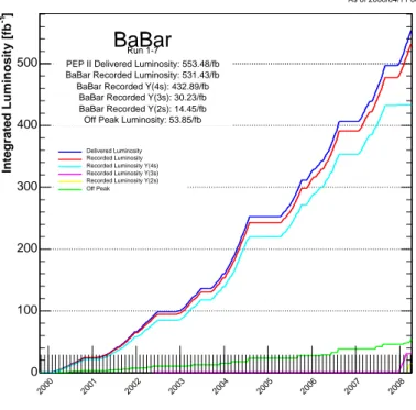
From December 2007 until February 2008, PEP-II operated at the resonance of Υ(3S), taking 30 fb−1 of data. In the very last period, just before the final shutdown, a scan of
other Υ resonances, up to Υ(5S), was performed. Data taking ended in April 2008 with a total recorded luminosity of 531 fb−1.
In PEP-II, the electron beam of 9 GeV collides head-on with the positron beam of 3.1 GeV resulting in a Lorentz boost for the Υ(4S) of βγ = 0.56 in the laboratory frame. The asymmetry of the machine is motivated by the need of separating the decay vertexes of the two B mesons, a crucial point for the determination of the CP asymmetries. The boost allows the separation and reconstruction of the decay vertexes of both B mesons, the determination of their relative decay length measured in the center-of-mass frame, the difference of their decaying time and thus the measurement of time dependent asymmetries. Nevertheless other stringent requirements on the detector are placed in order to measure the very small branching ratios of B mesons to CP eigenstates:
- large and uniform acceptance down to small polar angles relative to the boost direc-tion;
- excellent reconstruction efficiency down to 60 MeV/c for charged particles and 20 MeV for photons;
- very good momentum resolution to separate small signals from background;
- excellent energy and angular resolution to detect photons coming from π0 and η
decays, and from radiative decays in the range from 20 MeV to 4 GeV;
- very good vertex resolution, both transverse and parallel to the beam direction;
- efficient electron and muon identification, with low misidentification probabilities for hadrons. This feature is crucial for tagging the B flavor, for the reconstruction of charmonium states and also important for the study of decays involving leptons;
- efficient and accurate identification of hadrons over a wide range of momenta for B flavor-tagging and for the reconstruction of exclusive states;
- low-noise electronics and a reliable, high bandwidth, data-acquisition and control system;
- detailed monitoring and automated calibration;
- an on-line computing and network system that can control, process and store the expected high volume of data;
- detector components that can tolerate significant radiation doses and operate reliably under high background conditions.
2.1
The PEP-II Asymmetric Collider
The PEP-II B factory is part of the accelerator complex at SLAC, shown in Figure 2.1. The electron beam is produced by the electron gun near the beginning of the two-mile long linear accelerator (the “linac”). The gun consists of a thermally heated cathode filament held under high voltage. Large numbers of electrons are “boiled off” the cathode,
accelerated by the electric field, collected into bunches, and ejected out of the gun into the linac. The electron bunches are accelerated in the linac with synchronized radio-frequency (RF) electromagnetic pulses generated in RF cavities through which the beam passes by a series of 50 Megawatt klystron tubes (klystrons generate the pulses with their own lower energy electron beams passing through resonant cavities). The steering, bending, and focusing of the beam is carried out with magnets throughout the acceleration cycle.
Figure 2.1: A schematic depiction of the B factory accelerator complex ad SLAC.
After acceleration to an energy of approximately 1 GeV, the electron beam is directed to a damping ring, where the beam is stored for some time. As it circulates in the ring, it loses energy through synchrotron radiation and is continuously re-accelerated by RF cavities. The radiation and careful re-acceleration has the effect of reducing the emittance, or spatial and momentum spread of the beam, a necessary step in high-luminosity collisions. The “damped” beam is then re-directed to the linac and accelerated to 8.9 GeV.
Half of the generated electron bunches are used for the generation of the positron beam. They are accelerated to approximately 30 GeV, extracted from the linac and directed onto a tungsten target, producing electromagnetic showers that contain large numbers of electron-positron pairs. The positrons are separated electromagnetically from the electrons, collected into bunches, accelerated, and sent through the return line to the source end of the linac. The positron beam is then accelerated and shaped like the electron beam through the linac and its own damping ring, culminating in an energy of 3.1 GeV.