Università Degli Studi Di Catania
Dipartimento Di Scienze Fisiche Ed Astronomiche
Dottorato di Ricerca in Fisica – Ciclo XXXI
________________________________________________________
Ph.D. Thesis
Coupled Molecular Dynamics and Finite Element
Methods for the simulation of interacting
particles and fields
Ph.D. Student: Michele Cascio Tutor: Prof. Giuseppe Falci Co-tutor: Dott. Antonino La Magna Coordinator: Prof. Vincenzo Bellini
iii
Index
List of abbreviations pag. 1
Preface pag. 3
Chap. 1 Electromagnetic forces on dielectric particles immersed in a dielectric
medium pag. 9
1.1 Force on an electric dipole pag. 10
1.2 Effective moment of a dielectric particle pag. 12
1.3 Standard Dielectrophoretic force pag. 14
1.3.1 Application potential of DEP pag. 17
1.3.2 Clausius-Mossotti factor and
Standard DEP force pag. 21
1.3.3 Velocity field induced by DEP force pag. 22
1.4 DEP force calculated by the Maxwell Stress Tensor pag. 25
1.5 Remarks pag. 31
Chap. 2 Many pareticles thoeries of the electromechanical systems pag. 32 2.1 Mean field approach to many e.mec. particles kinetics pag. 33
2.1.1 Detrapping effects pag. 35
2.1.2 Cluster formation pag. 41
2.2 Analysis of stable configurations of e.mec. systems pag. 49 2.2.1 Monte Carlo study of the static configurations pag. 49 2.2.2 MST calculations of forces in few particles systems
iv
2.3 Conclusions pag. 58
Chap.3 The variational approach for the numerical solution of Partial Differential
Equations pag. 60
3.1 Partial Differential Equations pag. 61
3.2 Boundaries value problems pag. 62
3.2.1 Boundary problem for the Poisson equation pag. 63
3.3 Variational method pag. 66
3.3.1 Solution of Laplace’s problem by variational
method pag. 70
3.4 FEM approximation pag. 73
3.4.1 Galerkin Method of FEM approximation pag. 74
3.5 FEniCS project, Gmsh, Salome pag. 75
3.5.1 FEniCS project pag. 75
3.5.2 Gmsh pag. 77
3.5.3 Salome pag. 78
3.6 Remarks pag. 80
Chap. 4 Coupled Molecular Dynamics-Finite Element Method algorithm pag. 81
4.1 Molecular Dynamics pag. 82
4.1.1 MD implementation pag. 83
4.2 Verlet integration pag. 86
v
4.2.2 Velocity Verlet algorithm pag. 89
4.3 MD-FEM algorithm pag. 92
4.4 Conclusions pag. 97
Chap. 5 Simulated evolution of EMPs’ systems pag. 98
5.1 Single particle external interactions pag. 100
5.2 Particle Model pag. 104
5.3 Model validation for simple configurations pag. 108
5.4 MD-FEM simulation results in many particle systems pag. 113
5.4.1 Case (a): MDA-MD-231 cells pag. 116
5.4.2 Case (b): two cells system MDA-M231 and
B-Lymphocites pag. 127
5.5 Geometry’s effects pag. 134
5.5.1 Case (c): MDA-MD-231 cells pag. 134
5.5.2 Case (b): two cells system MDA-M231 and
B-Lymphocites pag. 136
5.6 Conclusions pag. 138
Chap. 6 Generalization of the MD-FEM formalism for particles of generic
shape pag. 140
6.1 Rigid-body dynamics pag.140
6.2 Quaternions pag. 142
6.2.1 Algebra of quaternions pag. 144
vi
6.3 Rotational Velocity Verlet pag. 147
6.4 Control instruction in simulations of rotational motion of non-spherical
particles pag. 150
6.4.1 Overlap between particles pag. 151
Conclusions pag. 154
Appendix A. Field due to a finite dipole pag. 157
Appendix B. Effective dipole moment of a dielectric particle pag. 160 Appendix C. Circulating Tumoral Cells and microfluidics technology
pag. 164
C.1 Circulating Tumoral Cells pag. 164
C.1.1 Metsastasis pag. 165
C.1.2 CTCs analysis as a “liquid biopsy” pag 167 C.1.3 CTCs in breast cancer patients. MDA-MB – 231 cell
line pag. 169
C.1.4 Techniques of CTCs isolation pag. 170
C.2 Microfluidics Technology pag. 173
Appendix D. Particle model pag. 178
Appendix E.MD-FEM code details pag. 182
E.1 Mesh generation pag. 182
E.2 Finite elements and Funcion Space generation pag. 183
vii
E.4 Solution of Laplace’problem pag. 185
E.5 Control instructions pag. 186
E.5.1 Particle-wall interaction pag. 186
E.5.2 Overlapping between particles pag. 187
Appendix F. Re{𝑓𝐶𝑀} of MDA-MB231 cells and Lymphocites pag. 190
References pag. 194
List of pubblications and conference participations pag. 212
1
List of abbreviations
AC alternating current CM Clausius-Mossotti CTCs Circulating Tumor Cells DC direct current
DEP dielectrophoresis e.mec. electromechanical e.m electromagnetic
EMPs Electromechanical Particles FEM Finite Element Method LOC Lab-On-a-Chip
MC Monte Carlo
MEMS Micro Electro-Mechanical Systems MD Molecular Dynamics
MD-FEM Molecular Dynamics - Finite Element Method MST Maxell Stress Tensor
n-DEP negative - DEP p-DEP positive - DEP
3
Preface
The dynamical simulation of many particle systems is currently a widespread technique in many fields: e.g. nuclear and atomic physics, computational materials science, computational chemistry, molecular biology and pharmacology. Under the locution “Molecular Dynamics” (MD) we can regroup a variety of approaches and numerical codes, whereas the commonalities are: 1) the atomistic (or nuclear) resolution (i.e. particles are atoms or nucleons), 2) the force derivation, starting from the systems’ configuration, through semi-classical (also called semi-empirical) or quantum mechanics based theoretical frameworks, 3) the (generally explicit) numerical integration of the Newton-like equations of motion to simulate the system kinetics. Within this scheme methodology variations can be found in the literature, but it is undoubtedly valid to qualify the MD meaning in the field of the scientific computation.
The general scope of this Thesis work is the extension of the MD methods to the study of the kinetics of larger particles (i.e. from mesoscopic dimensions and above), where effective particle-particle interactions are mediated by a field evolving self-consistently with the many particles
system. This objective is mainly motivated by the applications of the
method to control and predict the manipulation of mesoscopic (electrically) neutral particles by means of electromagnetic (e.m.) interactions: i.e. exploiting the so called dielectrophoresis (DEP) phenomena in the systems of electromechanical particles (EMPs). This is the specific case of study
4 here considered, but in principle the methodology can applied after suitable adaptation to also other systems.
In the particular case of the DEP driven systems, which will be briefly introduced in the following, we believe that our modelling approach satisfies the requirement of the general accurate prediction of the kinetics evolution; whilst previous theoretical approaches have several limitations which limit the applicability only under particular conditions.
Applications of DEP range from bio-structure assembling [1, 2] and nanostructure deposition (e.g. nanocluster, nanowires or nanotube) [3] to filtering systems [4]. A branch of emerging applications is related to the controlled manipulation of micro and nano-sized particles dispersed in colloidal solutions (i.e. biological particles such as cells or DNA), since the strong selectivity of the response depends on the particle volume, shape and composition [5, 6]. In fact, the forces exerted by non-uniform AC electric fields, due to the frequency dependent responses, can be used to move and manipulate polarizable microparticles (such as cells, marker particles, etc.) suspended in liquid media. The DEP allows manipulation of suspended particles without direct contact: this is also significant for many applications in micro Total-Analysis Systems (TAS) technology [7]. Manipulation includes cell partitioning/isolation [8] for the capture/separation without the use of biomarkers: in fact, cells can be collected, concentrated, separated and transported using the DEP forces arising from microelectrode structures having dimensions of the order of 1 to 100 μm [5]. One of the core strengths of DEP is therefore that the characterization of different cells depending only on the dielectric properties controlled by the particle’s individual phenotype; hence, the process does not require specific tags or involve
5 chemical reactions. The DEP based on AC electro-kinetics has recently been given more attention in microfluidics [9] due to the development of novel microfabrication techniques. In a typical device for the capture/separation of cells, the non-uniform field for the generation of the DEP force, responsible for the particle’s manipulation and control, is imposed by microelectrodes patterned on substrates (typically of glass) using fabrication techniques borrowed from Micro-Electro-Mechanical Systems (MEMS) [7]. The electric field is applied through the electrodes present in a microfluidic channel and the fluid flows through it.
As we will discuss in detail in Chapter 1, direct and rather straightforward numerical solutions of EMPs’ kinetics can be obtained when the following approximations (which we can indicate as single particle
approximation) are considered: a) diluted limit (i.e. negligible effective
particle-particle interactions), b) point-like particles (i.e. neglecting steric interactions), c) large distance between the particles and the source of the electric field (electrodes). This theory could be used to estimate roughly the EMPs’ [10, 11, 12]; however, in many real conditions these approximations are not verified and DEP is an example of field mediated force which can in principle induce a complex many particle behavior. Indeed, the forces acting on the particles depend in the general case on the overall system configuration since polarization alters locally the field which can be barely approximated by the external field generated by the sources. As a consequence, predictive theoretical studies of this large class of systems could be only possible thanks to the development of real-system models and numerical simulations. In order to study EMPs beyond the single particle approximation, computational studies of the DEP driven systems in
6 particular conditions have been recently presented in the scientific literature and they will be briefly presented in Chapter 2. In particular: stable configurations of particles dispersed in a static fluid [13] have been determined using Monte Carlo methods [14]; numerical models and simulations of the movement of cells in a moving fluid within a microfluidic channel introducing many-particle effects in the mean field approximation [15, 16] have been derived; finally, exact calculations of the forces by means of commercial tools [17] in the few-particles case have been reported.
Our contribution [18] aims to fully overcoming the single particle approximation, focusing on the theoretical study (see Chapters 4, 5 and appendices for the formalization of the method) of the dynamics of EMPs suspended in a colloidal solution in the presence of a non-uniform variable electric field. Our numerical simulations of a three-dimensional (3D) model system aim at providing predictions of both stable configurations of the particles and their dynamics in fully three-dimensional configurations, minimizing the approximations usually considered in models of mutual interactions. As a case of study, presented in Chapter 5, a system has been chosen consisting of biological cells dispersed in a colloidal solution (of which the typical characteristics of interest are reported in the literature) that flows into a microfluidic channel in the presence of e.m. fields.
3D simulations of DEP phenomena are rather rare in the literature, as they require large computational resources; moreover, most 3D DEP models are based on particles in the already discussed diluted solution limit. Nevertheless, in real applications, particle manipulation and characterization using dielectrophoresis are generally performed in a confined region close to
7 the electrodes, so that the interaction between the particles and the surrounding walls can be significant. Here we run a detailed study, with a non-approximate calculation of the forces, which are estimated by integrating the Maxwell Stress Tensor over the surfaces of the particles [19]. The dynamics are simulated by techniques borrowed from Molecular
Dynamics (MD), which, as stated above, is a simulation method that has
been successfully applied in the atomistic simulation field [20], whilst the
Finite Element Method (FEM) is applied to obtain self-consistent numerical
solutions of the partial differential equations regarding the e.m. field. The Coupled MD-FEM algorithm and its implementation in the FEniCS environment are also presented in the theoretical sections. The examples of the method’s application will focus on DEP induced translation of spherical particles (in particular a dielectric model of: MDA-M231 tumor cells, B-Lymphocites and mixtures of them), however after suitable adaptation it can be applied in more general cases (i.e. non-spherical particles, roto-translation, mixed DEP and conventional electrophoresis).
After validation of the FEniCS developer team, the numerical code simulating EMPs kinetics by means the cited coupled MD-FEM methodology is distributed as an open source tool at the web page:
https://bitbucket.org/barolidavide/tumor_detection_dolfin/src/master/. Open source distribution is possible thanks to the use of supporting frameworks (namely: FEniCS [21] for the PDE solutions, Gmsh [22] for the meshing and Salome for the graphical analysis) which are covered by GPL and/or LGPL licenses. The main modules are: a) the MD related routines, b)
8 the interface with Gmsh for the automatic meshing of the system configurations, c) the FEniCS interface for the force evaluation. The modules have been implemented from the scratch in the Python language while parallelization of the code has been obtained in an MPI environment.
9
Chapter 1
Electromagnetic forces on dielectric particles
immersed in a dielectric medium
Particles with sizes that range from sub-micrometers to about one millimeter and with particular electrical and/or magnetic properties experience mechanical forces and torques when they are subjected to electromagnetic (e.m.) fields. Particles of this type are called “electromechanical particles” (EMPs) [23]. Mutual interactions between EMPs could also occur when they are close enough to modify the force field obtained in the isolated particle limit.
One of the phenomena that affect electromechanical (e.mec.) particles is the “dielectrophoresis” (DEP), which describes the force exerted by a non-uniform electric field on polarizable neutral particles [23]: in a uniform electric field, neutral particles experience the polarization (an electric dipole is induced) which does not cause acceleration, whereas in a non-uniform electric field the forces due to polarization are not balanced and motion occurs: the net force is directed towards areas with either a higher or a lower electric field intensity, depending on the polarization properties of the particle and the background medium. Herbert Pohl’s first scientific publication defines DEP as “the natural movement of neutral bodies caused by polarization in an uneven electric field” [24].
In this chapter we will resume the theory of the e.m. forces deriving some concepts and expressions used in the next chapters. The following
10 themes will be presented: the formulation for the electromagnetic force acting on an electric dipole immersed in an external electric field, the concept of the effective dipole moment of a polarized particle, the standard (approximate) dielectrophoretic force acting on a particle and the more accurate dielectrophoretic force calculated by the use of the Maxwell Stress Tensor.
1.1 Force on an electric dipole
A finite dipole consists in two-point charges +q and –q separated by a vector distance 𝒅. In the limit where |𝒅| → 0 and 𝑞 → ∞ such that the 𝑞𝑑 product remains finite, the point dipole is defined. We consider in the following discussion a dipole with a finite spacing between the two charges, immersed in a non-uniform electric field 𝐄(𝒓) which includes no contributions due to the dipole itself. The dipole moment is defined as follows:
𝐩 = 𝑞𝒅. (1.1)
In general, the two charges experience different values of force and the dipole will be subject to a net force equal to:
𝐅 = 𝑞𝐄(𝒓 + 𝒅) − 𝑞𝐄(𝒓), (1.2)
11 Fig. 1.1 A small dipole in a non-uniform electric field.
If |𝒅| is small compared to the characteristic dimension of the electric field nonuniformity, 𝐄 can be expanded about position 𝒓 using the Taylor series expansion:
𝐄(𝒓 + 𝒅) = 𝐄(𝒓) + 𝒅 ∙ ∇𝐄(𝒓) + ⋯ (1.3)
By replacing Eq. (1.3) in Eq. (1.2):
12 In the limit |𝒅| → 0 but such that 𝐩 remains finite, neglecting terms of the order greater than the first and substituting the definition of Eq. (1.1) in Eq. (1.4), the force on a dipole results:
𝐅𝑑𝑖𝑝= [𝐩 ∙ ∇]𝐄(𝒓). (1.5)
The dipole therefore experiences a net force only if the external imposed electric field is non-uniform. Eq. (1.5) represents an approximation for the force exerted on any physical dipole, such as a polarized particle of finite size. The approximation used is called dielectrophoretic approximation [23].
1.2 Effective moment of a dielectric particle
In the derivation of Eq. (1.5), no reference is made to the nature of the dipole moment 𝐩, which can be the permanent moment of a polar particle or might be induced in a particle by an imposed electric field. In this Thesis, the latter case is considered. In general, the moment-induced field depends on both externally imposed and mutual field contributions (due to the presence of other particles).
The moment must relate to the electric field and to the particle parameters so that it can be used in Eq. (1.5). It is fundamental to identify the correct expression for the dipole moment to be used in formulation for the force (Eq. (1.5)) in the case of polarized particle. It is consequently useful to introduce the concept of effective dipole moment, 𝑝𝑒𝑓𝑓. The
13 defined as the moment of an equivalent, free-charge point dipole that causes the same dipolar electrostatic potential if it is immersed in the same medium and occupies the same position as the center of the particle.
The electrical potential Φ𝑑𝑖𝑝, due to a finite dipole centered in the origin of a Cartesian reference system and aligned with the z axis, immersed in a linear dielectric medium of permittivity 𝜀𝑚, in the point with coordinates (𝑟, 𝜗), radial and polar respectively, assumes the following form (see Appendix A):
Φ𝑑𝑖𝑝(𝑟, 𝜗) =
𝑞𝑑𝑐𝑜𝑠𝜗
4π𝜀𝑚𝑟2 . (1.6)
As a consequence, the formula of the electric potential produced by the polarized dielectric particle will contain the effective moment instead of the term 𝑞𝑑:
Φ(𝑟, 𝜗) =𝑝𝑒𝑓𝑓𝑐𝑜𝑠𝜗
4π𝜀𝑚𝑟2. (1.7)
The expression of 𝑝𝑒𝑓𝑓 for the case of a spherical particle is
presented below. Consider an isolated homogeneous dielectric particle of radius R, permittivity 𝜀𝑝 and conductivity 𝜎𝑝, immersed in a dielectric fluid
medium of permittivity 𝜀𝑚 and conductivity 𝜎𝑚. The particle and the medium are therefore characterised by the ohmic conductivity with no dielectric loss.
14 The calculated potential of the sphere can be expressed in the form of Eq. (1.7); and indicating with 𝐄 the electric field in which the dipole is immersed, the effective moment is (see Appendix B):
𝐩𝑒𝑓𝑓 = 4π𝜀𝑚𝑓𝐶𝑀𝑅3𝐄 , (1.8)
where
𝑓𝐶𝑀 = 𝜀̃𝑝−𝜀̃𝑚
𝜀̃𝑝+2𝜀̃𝑚 (1.9)
is the so-called Clausius-Mossotti factor, which contains the complex dielectric constants of the particle and of the medium, defined as it follows (see Appendix B): 𝜀̃𝑚 = 𝜀𝑚− 𝑖𝜎𝑚 𝜔, (1.10.a) 𝜀̃𝑝 = 𝜀𝑝− 𝑖 𝜎𝑝 𝜔. (1.10.b)
𝑓𝐶𝑀 is therefore a complex quantity, dependent on the angular frequency 𝜔.
1.3 Standard Dielectrophoretic force
The discussion carried out in the previous sections reveals implications for the so-called ponderomotive force exerted by a non-uniform electric field upon dielectric materials.
15 It is assumed that the motion of EMPs is induced by a sinusoidally time-varying and non-uniform electric field and consequently exponential notation can be used [25]:
𝐄(𝒓, 𝑡) = Re{𝐄(𝒓)𝑒−𝑖𝜔𝑡}. (1.11)
By replacing in Eq. (1.5) 𝐩 with 𝐩𝑒𝑓𝑓 and 𝐄(𝒓) with the expression of the electric field of Eq. (1.11), the time dependent force acting on the dielectric particle, called Standard DEP force and here indicated with 𝑭𝑆𝑇𝐷, is obtained:
𝑭𝑆𝑇𝐷=[𝐩
𝑒𝑓𝑓∙ ∇]𝐄(𝒓, 𝑡). (1.12)
This force consists of a constant average component and a time-varying term. The latter term is usually damped because of the viscosity of the suspension medium in the cases of particles with size in the range from 1 to 1000 μm. Consequently, the only relevant term is the one averaged over time. Starting from the previous equation, this term can be written [1]:
〈𝑭𝑆𝑇𝐷〉 =1
2Re{[𝐩𝑒𝑓𝑓∙ ∇]𝐄
∗(𝒓)} (1.13)
where 〈 〉 indicates the time-average and the asterisk indicates the complex conjugation. By inserting Eq. (1.8) in Eq. (1.13), using the vector identity:
16 and the condition ∇ ∧ 𝐄 = 0 (irrotationality of the field 𝐄), the force assumes the form:
〈𝑭𝑆𝑇𝐷〉=2π𝜀
𝑚Re{𝑓𝐶𝑀}𝑅3∇(|𝐄𝑅𝑀𝑆|2), (1.14)
where 𝐄𝑅𝑀𝑆 is the root mean square of electric field.
The Eq. (1.14) predicts the fundamental phenomenology of dielectrophoresis relative to spherical dielectric particles. The following are the main characteristics of the dielectrophoretic force acting on a lossless dielectric spherical particle immersed in a lossless medium:
the intensity of 〈𝑭𝑆𝑇𝐷〉 is proportional to particle volume, 𝜀 𝑚,
Re{𝑓𝐶𝑀} and ∇(|𝐄𝑅𝑀𝑆|2);
the sign of 〈𝑭𝑆𝑇𝐷〉 depends upon the sign of Re{𝑓 𝐶𝑀};
depending on Re{𝑓𝐶𝑀}, by Eq.s (1.9), (1.10a) and (1.10b) it follows that 〈𝑭𝑆𝑇𝐷〉 depends on the frequency;
particles experience a DEP force only when the electric field is non-uniform;
〈𝑭𝑆𝑇𝐷〉 does not depend on the polarity of the electric field and is
17 the 〈𝑭𝑆𝑇𝐷〉 vector is directed along ∇(|𝐄
𝑅𝑀𝑆|2) and therefore can
have any orientation with respect to the electric field vector;
DEP is usually observed for particles with diameters ranging from approximately 1 to 1000 μm.
1.3.1 Application potential of DEP
〈𝐅STD〉 depends on the shape and size of the particle, the intensity and
frequency of the oscillating electric field and the dielectric properties of the particle and medium. A distinction can be made between positive
dielectrophoresis (p-DEP) and negative dielectrophoresis (n-DEP), defined
as follows:
a) p-DEP: Re{𝑓𝐶𝑀} > 0, particles are attracted toward the electric field
intensity maxima and repelled from the minima;
b) n-DEP: Re{𝑓𝐶𝑀} < 0, particles are attracted toward electric field
intensity minima and repelled from the maxima.
Re{fCM} represents the effects of the arrangement of electrical charges, depending on the permittivity and conductivity values of the particle and the medium. Phenomenology is explained as follows. When a particle is suspended in a medium (typically an electrolyte) in the presence of an
18 electric field, the charges inside the particle and inside the medium will be redistributed at the particle-medium interface depending on their polarizability. Two cases can be distinguished, corresponding to the previous definitions a) and b) respectively:
A) the polarizability of the particle is higher than that of the medium: an excess of charge will accumulate at the particle’s side;
B) the polarizability of the medium is higher than that of the particle: an excess of charge will accumulate at the medium’s side.
In both cases, the resulting charge distribution is non-uniform and involves a difference in the charge density on either side of the particle. An induced dipole across the particle, aligned with the applied electric field, is therefore generated. When the particle-medium system is in the presence of a non-uniform electric field, the particle feels different forces at each end. Figure 1.2 shows this situation in an example where a pair of electrodes of different shape generates a non-uniform electric field. The difference in force at both ends generates a net force with direction depending on the polarizability of the particle and the medium.
19 Fig. 1.2 (a): Field lines of a non-uniform electric field generated by a pair of electrodes with different shape. (b) and (c): Dielectric particle in a medium in the presence of the non-uniform electric field (the field lines are not shown); the arrows indicate the forces acting on the charge distributions; the width of the arrows indicates the intensity of the forces; qualitative electric charge arrangements at the particle-medium interface are shown. In (b) the dielectric parameters of the particle and the medium result in Re{𝑓𝐶𝑀} > 0 and the electric charge arrangement generates p-DEP, with a net force directed towards the electric field intensity maxima. In the case (c) instead Re{𝑓𝐶𝑀} < 0 and n-DEP is generated, with a net force directed towards the electric field intensity minima.
Due to all its characteristics, the DEP force allows the control and manipulation of particles of micrometric size dispersed in colloidal solutions. It is very remarkable, for practical applications, the ability of DEP to induce both negative and positive forces. Thanks to this prerogative, the DEP force allows the separation of particles: in sorting operation mode, when two types of particles are present, the frequency can be chosen for the capturing and separations so as one cell type experiences n-DEP moving away from the electrodes, and the second type experiences p-DEP, moving towards the electrodes, as can be seen in Eq. (1.14).
20 As will be seen in Chap. 5, the control/separation by DEP of particles dispersed in a liquid medium will be the subject of computational studies in this Thesis.
21
1.3.2 Clausius-Mossotti factor and Standard DEP force
In this next section, further considerations on the link between 𝑓𝐶𝑀 and 〈𝑭𝑆𝑇𝐷〉 are given.
The explicit form of the Clausius-Mossotti factor is:
𝑓𝐶𝑀= 𝜀̃𝑝−𝜀̃𝑚 𝜀̃𝑝+2𝜀̃𝑚= 𝜀𝑝−𝜀𝑚−𝑖𝜎𝑝−𝜎𝑚𝜔 𝜀𝑝+2𝜀𝑚 −𝑖𝜎𝑝+2𝜎𝑚𝜔 . (1.15a)
The real and imaginary parts are:
Re{𝑓𝐶𝑀} = Re { 𝜀̃𝑝−𝜀̃𝑚 𝜀̃𝑝+2𝜀̃𝑚} = (𝜀𝑝−𝜀𝑚)(𝜀𝑝+2𝜀𝑚)−𝜔21(𝜎𝑚−𝜎𝑝)(𝜎𝑝+2𝜎𝑚) (𝜀𝑝+2𝜀𝑚) 2 +1 𝜔2(𝜎𝑝+2𝜎𝑚) 2 , (1.15b) Im{𝑓𝐶𝑀} = Im { 𝜀̃𝑝−𝜀̃𝑚 𝜀̃𝑝+2𝜀̃𝑚} = (𝜎𝑚−𝜎𝑝)(𝜀𝑝+2𝜀𝑚)−1 𝜔(𝜀𝑝−𝜀𝑚)(𝜎𝑝+2𝜎𝑚) (𝜀𝑝+2𝜀𝑚) 2 +1 𝜔2(𝜎𝑝+2𝜎𝑚) 2 . (1.15c)
It was seen by Eq. (1.14) that the sign of the time-average DEP force direction depends on the sign of Re{𝑓𝐶𝑀}, which contains all frequency dependence of the force. The frequency value at which Re{𝑓𝐶𝑀} becomes
zero is called the crossover frequency, 𝜈𝑐. By varying the frequency and exceeding this value, the force changes sign and the DEP response switches between n-DEP and p-DEP (or between p-DEP and n-DEP). From Eq. (1.15b), it can be seen that its form is:
22 𝜈𝑐 = 1 2𝜋√ (𝜎𝑚−𝜎𝑝)(𝜎𝑝+2𝜎𝑚) (𝜀𝑝−𝜀𝑚)(𝜀𝑝+2𝜀𝑚). (1.16)
The high- and low-frequency limits for Re{𝑓𝐶𝑀} are:
lim𝜔→∞Re{𝑓𝐶𝑀} = 𝜀𝑝−𝜀𝑚
𝜀𝑝+2𝜀𝑚, (1.17a)
lim𝜔→0Re{𝑓𝐶𝑀} = 𝜎𝑝−𝜎𝑚
𝜎𝑝+2𝜎𝑚. (1.17b)
From these expressions for the limits, it can be seen that DC conduction governs the low-frequency DEP behaviour, and dielectric polarization governs the high-frequency one. These conditions will be referred in Chap. 2.
1.3.3 Velocity field induced by the DEP force
Particles in colloidal solution in a liquid medium, which move under the action of the DEP force, undergo the effect of the drag force stemming from the viscosity of the medium. For a spherical object of radius R, in the case of a static fluid, the drag force is given by [26]:
𝑭𝑑𝑟𝑎𝑔 = 6𝜋𝜂𝑅𝒗, (1.18)
where 𝜂 is the dynamic viscosity and 𝒗 is the instantaneous velocity of the particle. Eq. (1.18) is referred as the Stokes law [27].
23 Assuming the validity of the single particle approximation, which is valid when the particles are far away from each other and from the electric field sources, it is possible to obtain each particle’s velocity field induced by DEP, here indicated by 𝒗𝐷𝐸𝑃. The DEP force is counterbalanced by the drag force due to the liquid if each particle subjected to the DEP force reaches very quickly a steady regime of motion [28] and, as a result, the electric and fluid components are completely uncoupled. By replacing 𝒗 with 𝒗𝐷𝐸𝑃 in
Eq. (1.18) and equating with the dielectrophoretic force of Eq. (1.14):
2π𝜀𝑚Re{𝑓𝐶𝑀}𝑅3∇(|𝐄𝑅𝑀𝑆|2) =6𝜋𝜂𝑅𝒗𝐷𝐸𝑃,
the following expression for the velocity field is obtained:
𝒗𝐷𝐸𝑃= 𝜀𝑚𝑅2Re{𝑓𝐶𝑀} 3𝜂 ∇(|𝐄| 2) = 𝜇 𝐷𝐸𝑃∇(|𝐄|2) , (1.19) where 𝜇𝐷𝐸𝑃 = 𝜀𝑚𝑅2Re{𝑓𝐶𝑀} 3𝜂 (1.20)
is the so-called “DEP mobility”.
In the case of a moving fluid, 𝒗 in Eq. (1.18) must be replaced with 𝒖 − 𝒗, being 𝒖 the local velocity of the fluid.
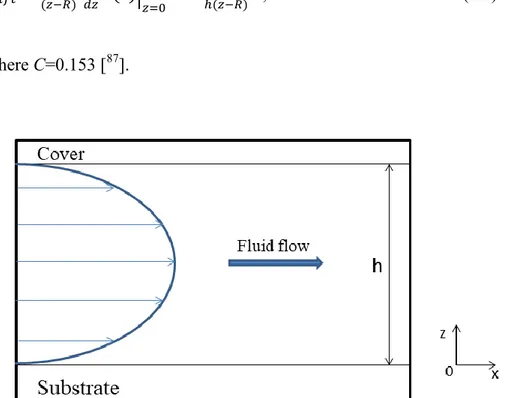
In DEP applications, microfluidic devices equipped with electrodes are often used (see Fig. 1.3 for a schematic from Ref. [6], while additional details on this type of device will be presented in Chapter 5) and the
24 expressions here derived are used to numerically evaluate an approximate kinetics of these systems of EMPs. Indeed, the velocity field of Eq. (1.19) can be determined by the numerical solution of the electric field equation and used to derive the trajectories of suspended particles, as shown in the example of Fig. 1.4 (from the Ref. [28]).
Fig. 1.2 Schematic of the model system of the DEP device. (Figure taken from: F. Aldaeus, Y. Lin, J. Roeraade, and G. Amberg, Electrophoresis 26, 2005).
Fig. 1.3 Particle trajectories in a medium liquid in the device operating in p-DEP condition only at the bottom of the channel. (Figure taken from: F. Aldaeus, Y. Lin, J. Roeraade, and G. Amberg, Electrophoresis 26, 2005).
25
1.4 DEP force calculated by the Maxwell Stress Tensor
The term “dielectrophoresis” is commonly used (and probably not correctly) to indicate two types of forces [23]:
the forces exerted upon individual noninteracting particles by an externally imposed nonuniform electric field;
the mutual attractive or repulsive force between two or more closely spaced particles.
The two types are basically related but distinctively observable. The first type of forces was the subject of the previous sections, while the second one will be detailed below.
In the models based on particles in the diluted solution limit (isolated particles), the first order dipole approximation, on which the Eq. (1.14) is based, is reasonable. This limit is valid in the case where particle-particle and particle-electrode interactions can be neglected (i.e. isolated particles). However, particle manipulation and characterization using DEP is generally performed in a confined region where particles accumulate and mutual forces occur, for example close to the electrodes of a Lab-on-chip device (See Appendix C.2). Including the mutual interactions in the definition of dielectrophoresis is therefore very important. For these reasons, an accurate approach for calculating the DEP forces is necessary: it is based on the rigorous application of the Maxwell Stress Tensor (MST, here and after indicated by 𝑇̿), that is described below.
26 The momentum change of a volume V of a dielectric inside an e.m. field can be correctly expressed as a surface integral of 𝑇̿ [25]:
𝑑
𝑑𝑡(𝑷𝑚𝑎𝑠𝑠 + 𝑷𝑓𝑖𝑒𝑙𝑑) = ∮ 𝑇̿ ∙ 𝑛̂𝑑𝛺𝛺 , (1.21)
where 𝑷𝑚𝑎𝑠𝑠 is the momentum of the mass contained in volume V, 𝑷𝑓𝑖𝑒𝑙𝑑 is the total e.m. momentum of the field, 𝛺 is the surface enclosing volume V and 𝑛̂ is the unit vector normal to 𝛺. According the e.m. field theory, the MST is given by the following general expression [29]:
𝑇̿ =1
2[𝐄 ⊗ 𝐃 + 𝐃 ⊗ 𝐄 + 𝐁 ⊗ 𝐇 + 𝐇 ⊗ 𝐁 − (𝐄 ∙ 𝐃 + 𝐁 ∙ 𝐇)𝐈], (1.22)
where E is the electric field, 𝐃 is the electric displacement, H is the magnetic field, 𝐁 is the magnetic induction, I is the unit tensor. Products with dot are scalar products, whereas the symbol ⊗ indicates a dyadic tensor product of vectors.
In this Thesis, the interest is focused on practical dielectrophoretic applications, where the applied external e.m. field generally has a frequency below 100 MHz and the correspondent field wave has a wavelength of the order of meters. This wavelength is much larger than dimensions of typical DEP arrangements. As a consequence, the contribution of the magnetic field can be neglected (near field approximation) and Eq. (1.22) becomes:
𝑇̿ = 1
27 If non-ferroelectric materials compose the EMPs, a linear dependence between 𝐃 and 𝐄 is valid and Eq. (1.23) becomes [30]:
𝑇̿ = Re{𝜀̃𝑚}[𝐄 ⊗ 𝐄 −1
2(𝐄 ∙ 𝐄)𝐈] , (1.24)
where 𝜀̃𝑚 is the complex permittivity of the medium (see Eq. (1.10a)).
The harmonic non-uniform electric field can be written [25]:
𝐄(𝐫, 𝑡) = Re{𝐄(𝐫)𝑒−𝑖𝜔𝑡} ≡1 2[𝐄(𝐫)𝑒
−𝑖𝜔𝑡+ 𝐄∗(𝐫)𝑒𝑖𝜔𝑡]. (1.25)
By replacing Eq. (1.25) in Eq. (1.24) and tacking the time average:
〈𝑇̿〉 = 1 2𝜋∫ 𝑇̿ 2𝜋 0 𝑑(𝜔𝑡) = =1 4Re{𝜀̃𝑚}[𝐄(𝐫) ⊗ 𝐄 ∗(𝐫) + 𝐄∗(𝐫) ⊗ 𝐄(𝐫) − |𝐄(𝐫)|2 𝐈]. (1.26)
By expressing in explicit form the dyadic products and the square module, Eq. (1.26) becomes: 〈𝑇̿〉 = 1 4Re{𝜀̃𝑚} ( 𝐸𝑥∗𝐸𝑥− 𝐸𝑦𝐸𝑦∗− 𝐸𝑧𝐸𝑧∗ 𝐸𝑥𝐸𝑦∗+ 𝐸𝑥∗𝐸𝑦 𝐸𝑥𝐸𝑧∗+ 𝐸𝑥∗𝐸𝑧 𝐸𝑦𝐸𝑥∗+ 𝐸𝑦∗𝐸𝑥 𝐸𝑦∗𝐸𝑦− 𝐸𝑥𝐸𝑥∗− 𝐸𝑧𝐸𝑧∗ 𝐸𝑦𝐸𝑧∗+ 𝐸𝑦∗𝐸𝑧 𝐸𝑧𝐸𝑥∗+ 𝐸𝑧∗𝐸𝑥 𝐸𝑧𝐸𝑦∗+ 𝐸𝑧∗𝐸𝑦 𝐸𝑧∗𝐸𝑧− 𝐸𝑥𝐸𝑥∗− 𝐸𝑦𝐸𝑦∗ ). (1.27)
From Eq. (1.21) it is noted that by integrating the MST over a surface external to the particle and infinitesimally close to it, we obtain the field-induced force acting on the particle itself (as the change of the moment
28 relative to the field is excluded). Therefore, if now we indicate with this particular surface, the time-averaged electromechanical force exerted on a particle immersed in a medium with complex permittivity 𝜀̃𝑚 and subject to
sinusoidal electric field E is [31, 32, 33]:
〈𝑭𝑀𝑆𝑇〉 = ∯ 〈𝑇̿〉 ∙ 𝑛̂𝑑𝛺
𝛺 . (1.28)
To identify the normal vector 𝑛̂ present in Eq. (1.28), the cosine directors are calculated using the following formulas:
cos(𝑟𝑥̂) = 𝑥−𝑥𝑐 √(𝑥−𝑥𝑐)2+(𝑦−𝑦𝑐)2+(𝑧−𝑧𝑐)2 , cos(𝑟𝑦̂) = 𝑦−𝑦𝑐 √(𝑥−𝑥𝑐)2+(𝑦−𝑦𝑐)2+(𝑧−𝑧𝑐)2 , cos(𝑟𝑧̂) = 𝑧−𝑧𝑐 √(𝑥−𝑥𝑐)2+(𝑦−𝑦𝑐)2+(𝑧−𝑧𝑐)2 .
From Eq. (1.28), the time-averaged DEP force exerted on the particle can therefore be written: 〈𝑭𝑀𝑆𝑇〉 = ( 〈𝐹𝑥𝑀𝑆𝑇〉 〈𝐹𝑦𝑀𝑆𝑇〉 〈𝐹𝑧𝑀𝑆𝑇〉 ) = ∯ 〈𝑇̿〉 ∙ 𝑛̂𝑑𝛺 = 𝛺 =1 4Re{𝜀̃𝑚} ∯ ( 𝐸𝑥∗𝐸𝑥− 𝐸𝑦𝐸𝑦∗− 𝐸𝑧𝐸𝑧∗ 𝐸𝑥𝐸𝑦∗+ 𝐸𝑥∗𝐸𝑦 𝐸𝑥𝐸𝑧∗+ 𝐸𝑥∗𝐸𝑧 𝐸𝑦𝐸𝑥∗+ 𝐸𝑦∗𝐸𝑥 𝐸𝑦∗𝐸𝑦− 𝐸𝑥𝐸𝑥∗− 𝐸𝑧𝐸𝑧∗ 𝐸𝑦𝐸𝑧∗+ 𝐸𝑦∗𝐸𝑧 𝐸𝑧𝐸𝑥∗+ 𝐸𝑧∗𝐸𝑥 𝐸𝑧𝐸𝑦∗+ 𝐸𝑧∗𝐸𝑦 𝐸𝑧∗𝐸𝑧− 𝐸𝑥𝐸𝑥∗− 𝐸𝑦𝐸𝑦∗ ) ∙ ( cos(𝑟𝑥̂) cos(𝑟𝑦̂) cos(𝑟𝑧̂) ) 𝑑𝛺 𝛺 (1.29)
29 The use of 〈𝑭𝑀𝑆𝑇〉, instead of 〈𝑭𝑆𝑇𝐷〉, allows the correct description in the
proximity of the electrodes when the particle-particle e.mec. interactions cannot be neglected due to the relatively large local density of EMPs. The usefulness of the calculation based on the MST consists also in its better applicability, compared with the dipole approximation method, to cases of objects with irregular shapes, such as nanowires, nanobelts etc.
The discussion presented for the calculation of 〈𝑭𝑀𝑆𝑇〉 can be
extended to the calculation of the time-averaged value of the torque, here indicated by 〈𝑻𝑀𝑆𝑇〉. By indicating with 𝒓 a vector connecting the reference
axis to the particle surface, the expression of the torque is:
〈𝑻𝑀𝑆𝑇〉 = ( 〈𝑻𝑥𝑀𝑆𝑇〉 〈𝑻𝑦𝑀𝑆𝑇〉 〈𝑻𝑧𝑀𝑆𝑇〉 ) = ∯ 𝒓 × 〈𝑇̿〉 ∙ 𝑛̂𝑑𝛺 = 𝛺 1 4Re{𝜀̃𝑚} ∯ 𝒓 × ( 𝐸𝑥∗𝐸𝑥− 𝐸𝑦𝐸𝑦∗− 𝐸𝑧𝐸𝑧∗ 𝐸𝑥𝐸𝑦∗+ 𝐸𝑥∗𝐸𝑦 𝐸𝑥𝐸𝑧∗+ 𝐸𝑥∗𝐸𝑧 𝐸𝑦𝐸𝑥∗+ 𝐸𝑦∗𝐸𝑥 𝐸𝑦∗𝐸𝑦− 𝐸𝑥𝐸𝑥∗− 𝐸𝑧𝐸𝑧∗ 𝐸𝑦𝐸𝑧∗+ 𝐸𝑦∗𝐸𝑧 𝐸𝑧𝐸𝑥∗+ 𝐸𝑧∗𝐸𝑥 𝐸𝑧𝐸𝑦∗+ 𝐸𝑧∗𝐸𝑦 𝐸𝑧∗𝐸𝑧− 𝐸𝑥𝐸𝑥∗− 𝐸𝑦𝐸𝑦∗ ) ∙ 𝛺 ( cos(𝑟𝑥̂) cos(𝑟𝑦̂) cos(𝑟𝑧̂) ) 𝑑𝛺. (1.30)
As it can be seen from Eq. (1.29) and Eq. (1.30), the calculation of the e.mec. force and torque requires the solution of the electric field, which in the case of practical dielectrophoretic applications derives from an applied electrical potential to the electrodes. In order to evaluate the electric field, the complex Laplace equation must therefore be solved. Again, the potential applied is time-varying and harmonic:
30
V(𝐫, t) = V(𝐫)𝑒𝑖𝜔𝑡 (1.31)
and the complex Laplace equation to be resolved is [34]:
∇ ∙ [𝜀̃ ∇ V(𝐫)] = 0. (1.32)
In Eq. (1.32), consider 𝜀̃ = 𝜀̃𝑚 inside the liquid medium and 𝜀̃ = 𝜀̃𝑝 inside the particles.
This equation is based on some assumptions: particle neutrality (negligible ion effect), harmonic oscillation (linear model) and negligible convection effects [35]. Moreover, as stated, the coupling of electric and magnetic fields can be neglected (∇ × 𝐄 = −𝜕𝐁
𝜕𝑡 = 0) and in this framework we can
derive the electric field simply as a gradient of the electrical potential:
31
1.5 Remarks
In this section we resume the formalism needed to evaluate (eventually using numerical methods) the force and torques in EMPs. We notice that for a spherical particle, the direct use of these expressions allows for a relatively simple derivation of the kinetics in diluted systems of EMPs. Anyhow, beyond the single particle approximation, such derivation could be strongly inaccurate. In the next chapter we present the state of the art (as it emerged at the beginning of the present Thesis work) of the theoretical/computational approaches for the study of many particle effects in a system of EMPs.
32
Chapter 2
Many-particle theories of
electromechanical systems
In this chapter we will briefly discuss the current state-of-the-art of the theoretical approaches to the study of many-particle effects in dielectrophoretic systems in order to discuss some limitations which we intend to overcome with our methodology. Firstly, we present the approaches in the continuum limit where particles are approximated as density fields. In this case, the multiparticle effects are highlighted by means of a medium field approach, while the formation of particle chains is analyzed according to reaction-diffusion models. Such approaches are independent of the calculation of the dielectrophoretic force.
The second part is dedicated to the more accurate particle-like description of the EMPs where, in turn, the limitations are related to the pure static configuration studied both with approximate dipole-dipole interactions and with the use of the Maxwell Stress Tensor for the derivation of the forces.
33
2.1 Mean field approach to many e.mec. particle kinetics
In dielectrophoretic devices, many-particle effects can arise due to the high concentration of particles in the surroundings of electrodes. This constitutes a substantial source of indetermination on the theoretical estimate of the trapping/separation efficiency when single particle solutions are used (see Section 1.3). An approximated method to include many-particle effects in the calculation of DEP trapping has been suggested [36], which is based on the Effective Medium Approximation (EMA) for electric parameters of the suspension [37].
As discussed in Chpt. 1, the Clausius–Mossotti factor (called also DEP spectrum) for a particle immersed in a medium is:
𝑓𝐶𝑀 = 𝜀̃𝑝−𝜀̃𝑚
𝜀̃𝑝+2𝜀̃𝑚. (2.1)
If the local particle density is high, the dipole-dipole particle interaction can significantly vary the DEP response [38] and consequently, the form of 𝑓𝐶𝑀. The mean field method consists on the correction of 𝑓𝐶𝑀, taking into account the many-particle effects as alteration of the medium complex dielectric. The correction is based on the EMA for the dielectric properties of heterogeneous two-component composite materials [15]. This approach allows calculating the electrical conductivity 𝜎 and the permittivity 𝜀 for various shapes of composite materials as a function of the hosted material (𝜀2, 𝜎2) and the host material (𝜀1, 𝜎1) properties. It is assumed that material
34 medium. The subscript p instead of 2 and m instead of 1 are used. The dielectric function is given by [15]:
𝜀(𝜑) =1 4[2𝜀𝑣− 𝜀𝑣 ′ + √(2𝜀 𝑝− 𝜀𝑝′) 2 + 8𝜀𝑚𝜀𝑝 ], (2.2) with 𝜀𝑣 = (1 − 𝜑)𝜀𝑚+ 𝜀𝑝𝜑, (2.3a) 𝜀𝑣′ = 𝜀𝑚𝜑 + (1 − 𝜑)𝜀𝑝. (2.3b)
where 𝜑 represents the volume fractions of cluster inclusions. The modification of 𝑓𝐶𝑀 (Eq. (2.1)) to include the EMA consists simply in these
substitutions:
𝜀𝑚 → 𝜀(𝜑), (2.4)
𝜎𝑚 → 𝜎(𝜑), (2.5)
In this way, the electrical properties of the mixture, composed of particles and liquid medium, are determined as a function of the volume fraction. The DEP mobility, defined in Eq. (1.20), becomes:
𝜇𝐷𝐸𝑃= 𝜀(𝜑)𝑅2Re{𝑓𝐶𝑀}
35 Figure 2.1 shows an example of a DEP spectrum obtained from experimental data on latex microspheres given in Ref. [39]:
Fig. 2.1 DEP spectrum of latex microspheres obtained from data given in Ref. [4]. Straight and dashed lines refer to the real and imaginary parts of the Clausius–Mossotti factor, respectively. (Figure taken from: O. E. Nicotra, A. La Magna, and S. Coffa, Appl. Phys. Lett. 93, 193902 (2008)).
The effect of EMA in the DEP spectrum is clear: both real and imaginary parts of the 𝑓𝐶𝑀 flat to zero as the volume fraction approaches to one.
2.1.1 Detrapping effects
The mean field approach allows the use of the same computational strategy of the single particle case presented in Chpt. 1. As a consequence, the electric potential V(𝐫) must be computed by solving the Laplace equation:
36 In a standard DEP simulation, the vector composition of the liquid medium velocity field 𝒖𝑚 with the particle’s velocity field 𝒗𝐷𝐸𝑃 gives all
information on the particle motion inside the DEP device, allowing to predict particle trajectories. 𝒖𝑚 is derived by the Navier–Stokes equation for
a steady and uncompressible fluid [40]. The total velocity field is:
𝒖𝑡𝑜𝑡= 𝒗𝐷𝐸𝑃+ 𝒖𝑚. (2.8)
𝒖𝑡𝑜𝑡 acts as a drift toward the electrodes and particles may therefore be represented by a drift-diffusion current 𝑱, as follows:
𝑱 = −𝐷∇𝜑 + 𝒖𝑡𝑜𝑡 𝜑. (2.9)
In the diluted limit and for particles’ dimensions in the micrometer scale, 𝐷 has the meaning of a numerical diffusion, introduced to stabilize the calculation, while for the high density case, 𝐷 can also effectively include the scattering event between particles or the limit threshold of 𝜑 for the packing. In order to prevent 𝜑 exceeding the threshold value for the packing fraction of 0.74, a diffusion coefficient D(𝜑) was introduced:
𝐷(𝜑) = 𝐷0
√1−0.74𝜑
, (2.10)
where 𝐷0 is a constant value to be fixed in order to take into account the diffusion due to particles crowding, especially at a high particle concentration regime.
37 The equation governing the time evolution of 𝜑 has a flux-conservative form:
∂𝜑
∂𝑡 = −∇ ∙ 𝑱. (2.11)
The set of Eqs (2.1)-(2.7) and (2.11) represent the governing equations to be solved. In this way, the local value of the volume fraction of dispersed particles is adjusted by drift-diffusion dynamics.
In Ref. [28] simulations were performed on a model with a particular geometry. The device modeled consists of a two-dimensional trap with an array of parallel interdigitated electrodes present at the base of a rectangular channel where the liquid medium flows. A schematic of the device, already presented in Section 1.3.3, is shown in Fig. 2.2.
Fig. 2.2 Schematic of the model system. (Figure taken from: F. Aldaeus, Y. Lin, J. Roeraade, and G. Amberg, Electrophoresis 26, 2005).
Spherical latex particles were considered, with radius R=5.87 𝜇𝑚 and the following dielectric constant and conductivity:
38 𝜀𝑝 = 2.4𝜀0,
𝜎𝑝 = 7.0 𝑆/𝑚2.
The liquid medium has the following specifications: 𝜀𝑚 = 78𝜀0,
𝜎𝑚 = 6.0 𝑆/𝑚2,
𝜂 = 10−3 𝑃𝑎 ∙ 𝑠𝑒𝑐.
The angular frequency is 10 KHz, 𝜑 = 0.3 and 𝐷0 = 9.6 10−9 𝑚2/𝑠.
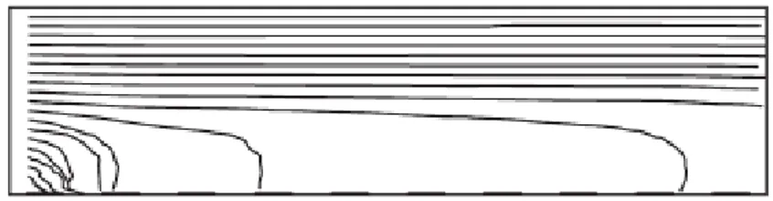
Figure 2.3 shows some snapshots of the solution at different values of time. The color field represents 𝜑 while red lines represent a set of particle trajectories which depart from the left side of the device. Electrodes (in number of 10) are taken at a voltage of 0 or +5 V in an alternate sequence.
39 Fig. 2.3 Snapshots taken at times 1, 2, 3, and 4 s (from upper to lower) regarding the time evolution of particle volume fraction 𝜑 (color field) and particle trajectories (red lines). The vertical color bar provides the correspondence between colors and values of 𝜑. Particles and fluid enter from the left, where at the boundary 𝜑 is fixed to 0.3, with initial fluid velocity of 15 𝜇𝑚. In the other boundaries the condition 𝑛̂ ∙ 𝑱 = 0 for Eq. (2.11) is assigned. (Figure taken from: O. E. Nicotra, A. La Magna, and S. Coffa, Appl. Phys. Lett. 93, 193902 (2008)).
As visible in the topmost part of Fig. 2.3, a complete trapping of the particles is predicted by the calculation when many-particle effects are neglected. Nevertheless, the self-consistency of the solution implies the change of the predicted trajectories of the particles. Indeed, as observed in the lowermost part of the same figure, the self-consistent solution indicates that some particle trajectories step away from the device. It is important to note that the many-particle effect is described by the real part of 𝑓𝐶𝑀: in particular, it diminishes as 𝜑 increases. In this condition, the many-particle effect in trapping efficiency becomes non-negligible. Furthermore, as described in Fig. 2.4, showing a small region around one electrode, the
40 trapping capabilities of the device is significantly reduced when the particle fraction surrounding the electrodes increases.
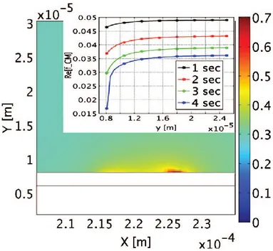
Fig. 2.4. An enlarged portion of snapshot at t=4 s of Fig. 2.3. The color field represents the particle volume fraction 𝜑 at the surroundings of an electrode where 𝜑 reaches its maximum value. Abscissa and ordinate are spatial coordinates. In the inner panel, the cross-section (taken just above the red region at 𝑥 = 2.26 10−4 𝑚) of the Clausius–Mossotti factor as a function of the ordinate is shown. Colors of the curves refer to the same times of the snapshots of Fig. 2.3. (Figure taken from: O. E. Nicotra, A. La Magna, and S. Coffa, Appl. Phys. Lett. 93, 193902 (2008)).
This aspect highlights the mutual influence between 𝜑 and the DEP spectrum as evidenced in the inset of the figure showing the dependence of 𝑓𝐶𝑀 on the y-coordinate near the electrode. As highlighted by these results, the influence of the many-particle effects on the features of DEP-based devices can be suitably investigated by combining EMA and drift-diffusion.
41 As discussed by the authors in Ref. [15], the many-particle correction is a fundamental tool to obtain reliable simulation outcomes in the prediction of trapping efficiency in the case of micro- and nanosized particles. This methodological approach is necessary when a high density of particles occurs near the electrode. This situation is rather common since high particle concentration can be achieved in device architectures where tight regions are designed to properly tailor the electric field [41].
2.1.2 Cluster formation
The diffusion formalism can be easily generalized to a reaction diffusion, as discussed in the following. In real systems with a large number of particles, the main effect of the induced electric dipole is the formation of particle clusters, particularly in the shape of chains of very different length, that align with the electric field (longitudinal chaining for identical particles) [42]. The clusters have different dielectrophoretic properties from those of their constituents: this is an aspect to be considered for the accurate description of the dielectrophoresis. In reference [43] it has been shown that particle-chain formation and evolution can be quantitatively described in a realistic device geometry. In this discussion, chains composed of no more than four particles are considered, however the approach followed can be easily generalized to a larger number of particles.
As seen in Chapter 1, the time-averaged force acting on a dipole in the presence of a non-uniform electric field
42 𝐄(𝐫, 𝑡) = 𝐄(𝐫)𝑒−𝑖𝜔𝑡
is:
〈𝑭𝐷𝐸𝑃(𝑡)〉 = 2π𝜀𝑚Re{𝑓𝐶𝑀}𝑅3∇(|𝐄𝑅𝑀𝑆|𝟐) (2.12)
where 𝐄𝑅𝑀𝑆 = 𝐄(𝐫)/√2 is the root mean square of electric field.
For a conducting particle in a DC field, 𝑓𝐶𝑀 is a real quantity depending
only on the electrical conductivities of the particle and the medium (see Eq. (1.17b)). For perfectly conducting particles in a liquid medium, namely in the limit:
𝜎𝑝
𝜎𝑚 → ∞, (2.13)
𝑓𝐶𝑀 tends to 1 by Eq. (1.17b). Assuming that particles are subjected only to
DEP and drag force and quickly reach a steady motion, the induced velocity field has the form of Eq. (1.19). For a spherical, perfect conductor particle of radius R2 immersed in a liquid of dynamic viscosity 𝜂, by Eq. (1.20) the
DEP mobility is:
𝜇𝐷𝐸𝑃= 𝜀𝑚𝑅22
3𝜂 .
Each type of chain is characterized by a well-defined DEP mobility 𝜇𝐷𝐸𝑃𝑖 ,
with i=1,2,3,4-particle chain. The total velocity field is: 𝒖𝑡𝑜𝑡𝑖 = 𝒗
𝐷𝐸𝑃 𝑖 + 𝒖
43 For the DEP mobility, the following relation in the steady motion is valid:
𝜇𝐷𝐸𝑃𝑖 = 𝛼𝑖𝜇𝐷𝐸𝑃1 , (2.15)
where 𝛼𝑖 (with i = 2,3,4) are essentially geometrical factors (𝛼2 = 6.8, 𝛼3 = 13.8, 𝛼4 = 23), also including the volume and shape enhancements of the
effective dipole moment of the i-particles chain. The particles and the chains can be represented using their particle volume fraction 𝜑𝑖 and drift-diffusion
current, defined as follows by generalizing Eq. (2.9):
𝑱𝑖 = −𝐷∇𝜑𝑖+ 𝒖 𝑡𝑜𝑡
𝑖 𝜑𝑖. (2.16)
Reaction terms 𝑄(𝑗)(𝑖), depending on the nature of the reaction considered, can be introduced for the description of the particle stitching and chain formation. By labeling each particle or particle-chain species with 𝑃𝑖, the stitching reactions with the associated rates are the following form:
2𝑃1 ↔ 𝑃2 → 𝑄(1)(2)= 𝑘1[𝑃1]2− 𝑘2[𝑃2], (2.17a) 3𝑃1 ↔ 𝑃3 → 𝑄(1)(3)= 𝑘3[𝑃1]2 − 𝑘4[𝑃3], (2.17b) 𝑃1+ 𝑃2 ↔ 𝑃3 → 𝑄(2)(3) = 𝑘5[𝑃1][𝑃2] − 𝑘6[𝑃3], (2.17c) 4𝑃1 ↔ 𝑃4 → 𝑄(1)(4)= 𝑘7[𝑃1]4− 𝑘 8[𝑃4], (2.17d) 2𝑃2 ↔ 𝑃4 → 𝑄(2)(4) = 𝑘9[𝑃2]2− 𝑘 10[𝑃4], (2.17e) 𝑃1+ 𝑃3 ↔ 𝑃𝑖 → 𝑄(3)(4) = 𝑘11[𝑃1][𝑃3] − 𝑘12[𝑃4], (2.17f)
44 where 𝑘𝑙 (𝑙 = 1, … , 12) are the reaction constants and [𝑃𝑖] are quantities proportional to the mass concentration. Providing [𝑃𝑖] → 𝜑𝑖, all 𝑘𝑙 are in
unit of 𝑠𝑒𝑐−1. The set of equations governing the reaction-diffusion
dynamics for 𝜑𝑖 is:
𝜕 𝜕𝑡𝜑 1+ ∇ ∙ 𝑱1 = −2𝑄 (1)(2)− 3𝑄(1)(3)− 𝑄(2)(3)− 4𝑄(1)(4)− 𝑄(3) (4), (2.18a) 𝜕 𝜕𝑡𝜑 2+ ∇ ∙ 𝑱2 = 𝑄 (1)(2)− 𝑄(2)(3)− 2𝑄(2)(4), (2.18b) 𝜕 𝜕𝑡𝜑 3+ ∇ ∙ 𝑱3 = 𝑄 (1)(3)+ 𝑄(2)(3)− 𝑄(3) (4), (2.18c) 𝜕 𝜕𝑡𝜑 4+ ∇ ∙ 𝑱4 = 𝑄 (1) (4) + 𝑄(2)(4)+ 𝑄(3)(4). (2.18d)
To consider larger chains, the corresponding equations must be added to the set of Eq. 2.18. Moreover, if 𝜇𝐷𝐸𝑃𝑖 and the stitching coefficients for larger
chains depend weakly on the number of particles in the chain, a compact set with a reduced number of differential equations can be used [44].
The overall set of governing equation to numerically simulate particle-chain formation is composed of Eq. (2.18), Eq. (7), 𝑬 = −∇ 𝑉 and the Navier-Stokes equation [16].
Many-particle corrections can be introduced, providing that: 𝜀1 → 𝜀(𝜑𝑡𝑜𝑡),
45 where 𝜑𝑡𝑜𝑡 = ∑4 𝜑𝑖
𝑖=1 is the total volume fraction. The dependence of 𝜀 on
𝜑𝑡𝑜𝑡 is based on the EMA used for transport simulation in DEP.
Simulations on unstructured and perfectly conducting particles dispersed in a saline solution are carried out in Ref. [16]. The dielectric parameters used are:
𝜀𝑚 = 78𝜀0,
𝜎𝑚 = 6 ∙ 10−4S/m.
For particles and chain: R=3.5 𝜇𝑚, 𝜀 = 𝜀0, 𝐷0 = 0.82 10−7 𝑚2/𝑠. The
device geometry is the same as that previously considered in Fig. 2.1. In the initial configuration, all the four particles volume fraction 𝜑𝑖 are equal to
zero and the reaction constants are set equal to: 𝑘1 = 2.1, 𝑘2 = 𝑘7 =
1.5, 𝑘3 = 𝑘8 = 𝑘10= 1.5, 𝑘4 = 1, 𝑘5 = 3.1, 𝑘6 = 1.8, 𝑘9 = 2.0, 𝑘11=
2.4, 𝑘12= 1.3.
𝑘𝑙 are free parameters to be adjusted in order to reproduce the real
particle-particle interaction. The choice of this simulation represents only an example of study in order to emphasize some typical aspects of the dynamics. In this sense this method needs a parameter calibration study with the aid of a more accurate particle-like approach.
Figure 2.5 shows the evolution for some time steps. Four DEP mobilities are considered because there are four kinds of objects.
46 Fig. 2.5. Panel (a): snapshots taken at times 0.2, 0.6, and 1.0 s (from upper to lower) showing the time evolution of the total particle volume fraction 𝜑𝑡𝑜𝑡 (see color bar on the right). Particles and fluid enter from the left boundary with a fluid speed of 0.5 𝜇𝑚/𝑠𝑒𝑐, where 𝜑1 is fixed to 0.3 and 𝜑2= 𝜑3= 𝜑4= 0. In the other boundaries the condition 𝜑𝑖∙ 𝑱𝑖= 0 is assigned. Electrodes (in number of ten) are separated from the fluid by a silicon layer 3 𝜇𝑚 thick and they are taken at a voltage of 0 or + 2.5 V in an alternate sequence. Panel (b): three-dimensional plot where both the colored surfaces and the height (z-axis) represent 𝜑𝑡𝑜𝑡 computed at times 0.6 and 1.0 s (from lower to upper) without particle stitching (𝜑𝑡𝑜𝑡 = 𝜑1 ). Panel (c): same as in panel (b) but with particle stitching included. (Figure taken from: O. E. Nicotra, A. La Magna, and S. Coffa, Appl. Phys. Lett. 95, 073702 (2009)).
The simulation time is reduced with respect to the one of the previous simulation where only spherical particles are considered. In fact, the DEP mobilities grow with increasing chain size and consequently a stronger DEP drift toward the electrodes is developed. This aspect can be seen in panels (b) and (c) of Fig. 2.5, where a calculation of 𝜑𝑡𝑜𝑡 without chain formation (𝑘𝑙 = 0) is also displayed for comparison.
In Fig. 2.6, showing the particle-chain formation, 𝜑1 and 𝜑2 are reported,
47 Fig. 2.6 Three-dimensional plot where the colored surfaces and the height (z-axis) represent respectively 𝜑1 and 𝜑2 taken at times 0.2, 0.5 and 1.0 s (from lower to upper). (Figure taken from: O. E. Nicotra, A. La Magna, and S. Coffa, Appl. Phys. Lett. 95, 073702 (2009)).
Fig. 2.7 Same as in Fig. 2.6 but for 𝜑3 and 𝜑4. Results shown refer only to time 1.0 s. (Figure taken from: O. E. Nicotra, A. La Magna, and S. Coffa, Appl. Phys. Lett. 95, 073702 (2009)).
48 In both Fig. 2.6 and Fig. 2.7, the volume fractions are represented by color field and height (z axis of the plot). Peaks are present in the colored surfaces at the edges of each electrode, where also the color field presents its maxima: this indicates that most part of the chain formation occurs in these regions. In fact, the rate terms in Eq. (2.17) are proportional to the volume fractions and particle stitching is more likely to occur in regions where particles accumulate. This mechanism, among others, is responsible for the slower kinetics of 𝜑3 and 𝜑4 with respect to 𝜑1 and 𝜑2.
The results of this simulation show the possibility of quantitatively describing particle-chain formation. This description is based on the extension of drift-diffusion dynamics with reaction terms properly included. The computation of the volume fractions 𝜑𝑖 allows to predict where and
when particle chain formation occurs in a dielectrophoretic device.
Regarding the DEP mobility, in general EMA tends to reduce it. DEP mobility instead increases due to particle-chain formation. There is a competition between these two many-particle effects, but the present simulation shows that the latter is favored on the basis of the shortening of the evolution time. The particle stitching in DEP seems thus to completely dominate the entire transport dynamics. The two simulations show the importance of the many-particle corrections. The design of a dielectrophoretic device should not neglect such a phenomenon.
49
2.2 Analysis of stable configurations of e.mec. systems
A different approach from that set out in the previous sections requires the evaluation of the external electric field. Section 2.2.1 describes a simulation based on the calculation, by the electric field, of the electric potential energy and on the use of the MC technique, whereas Section 2.2.2 describes a simulation based on the use of MST.
2.2.1 Monte Carlo study of the static configurations
The method presented in Ref. [45], described below, allows the simulation of sufficiently large systems in terms of size and number of particles (i.e. within the experimental scopes).
〈𝑭𝑆𝑇𝐷〉 is a non-conservative force which can however be calculated as the
negative gradient of the following effective average potential energy [46]:
𝑈̅𝑒𝑓𝑓(𝒓) = − 1
2𝛼𝑒𝑓𝑓𝐸𝑅𝑀𝑆
2 (𝒓), (2.19)
where 𝛼𝑒𝑓𝑓 is the average polarizability, which has the form:
𝛼𝑒𝑓𝑓 = 4π𝑅3Re{𝜀̃𝑚}Re{𝑓𝐶𝑀}.
The DEP force is approximated as those generated by the total distorted electric field, which is equal to the sum of the external field and the contributions of the dipoles induced in all the particles [47]:
50 𝐄𝑡𝑜𝑡(𝒓𝑖) ≈ 𝐄(𝒓𝑖) + ∑𝑎𝑙𝑙 𝑡ℎ𝑒 𝑝𝑎𝑟𝑡𝑖𝑐𝑙𝑒𝑠𝑗 𝐄𝑗(𝑟𝑖). (2.20)
By considering identical particles and neglecting multipole terms and mutual polarization, the effective potential energy can be derived from the expression that generalizes Eq. (2.19) for the case of particle-particle instantaneous interactions in the dipole approximation:
𝑈𝑖𝑗 ≈ − 1 2Re{𝐩𝑖(𝒓𝑖) ∙ 𝐄𝑗(𝒓𝑖) ∗} = −1 2Re{𝐩𝑗(𝒓𝑗) ∙ 𝐄𝑖(𝒓𝑗) ∗ }, (2.21)
where 𝐄𝑗(𝒓𝑖) is the electrical field generated by the dipole in the particle 𝑗 at
the position 𝒓𝑖, and 𝐩𝑖(𝒓𝑖) is the dipole moment induced on the i-th particle by the external field 𝐄(𝒓𝑖). Similar definitions apply to 𝐄𝑖(𝒓𝑗) and 𝐩𝑗(𝒓𝑗).
The dipole electric fields in Eq. (2.21) are:
𝐄𝑗(𝒓𝑖) = 1 4𝜋Re{𝜀̃𝑚} 3 𝐧 (𝐧∙𝐩𝑗)−𝐩𝑗 𝑅𝑖𝑗3 , (2.22) 𝐄𝑖(𝒓𝑗) = 1 4𝜋Re{𝜀̃𝑚} 3 𝐧 (𝐧∙𝐩𝑖)−𝐩𝑖 𝑅𝑖𝑗3 , (2.23) where 𝐧 =𝐑ij Rij.
Based on the above expressions, the average effective potential energy is:
𝑈̅𝑖,𝑗 ≅ 1 4𝜋Re{𝜀̃𝑚}|𝛼| 21−3 cos(𝜃𝑖𝑗 𝑖) cos(𝜃 𝑖𝑗 𝑗 ) 𝑅𝑖𝑗3 [𝑬𝑅𝑀𝑆(𝒓𝑖) ∙ 𝑬𝑅𝑀𝑆(𝒓𝑗)], (2.24)