High temperature (till 1500°C) contemporary thermal conductivity and thermal diffusivity measurements with the step flat heat source

(1)

High temperature (till 1500°C) contemporary thermal conductivity

and thermal diffusivity measurements with the step flat heat source

Gianluigi Bovesecchi

1

, Paolo Coppa

1 1

Dept. of Mec. Eng., Univ. of Rome “Tor Vergata”, Via del Politecnico 1, 00133 Rome (Italy)

e-mail:

gianluigi.bovesecchi@gmail.com

coppa@uniroma2.it

Keywords: high temperature, thermal conductivity, thermal diffusivity, step flat heat sorce

ABSTRACT

The method for contemporary measuring thermal conductivity, thermal diffusivity and thermal contact resistance up to 1500°C has been assessed. First the heat propagation model has been developed to be used in least square procedure to process temperature data and give the best estimate on the unknown parameters. Second special devices to be used in the experimental procedure have been designed and built or are going to be built. In the meanwhile ambient temperature tests on bricks have been carried out to establish the data processing procedure, and to recognize the experimental troubles likely to be found. These tests shows that the experimental data well follow the theoretical prediction, the thermophysical parameter can be evaluated with good accuracy, and that care must be taken to satisfying the theoretical assumptions on the base of the model, and to accurately process data for taking into account mutual dependence of the parameters

1. INTRODUCTION

Thermophysical properties of matter are considered essential to evaluate thermal behaviour of components both in steady state (above all thermal conductivity λ) and transient state (thermal diffusivity α). At high temperature (above 1000°C) these properties are fundamental in order to guarantee thermal insulation, or from the other point of view, good thermal contact. For instance, in rocket technology, a good thermal insulation around 1500°C is strongly required to improve the performances of the engine nozzle (this is one of the main reason of the present activity within an international cooperation agreement between the authors’ University and the Harbin Institute of Technology, Harbin, People Republic of China).

Among different methods to measure thermal conductivity and thermal diffusivity, the flat plane source methods, evolved in the hot strip method [1] [2], is well established, and supplies good results. Differently from other equally well established methods (probe method, for cylindrical samples, and flash method for flat thin samples), it can be used with bulk materials in many different shapes. Nevertheless, even if it has been applied at high temperature, further developments are required to solve some experimental and data processing problems. These problems can be summarizes as follows:

- the heat source and sample holders must be accurately designed, and built in material able to work at high temperatures, so it is suggested to realize them in ceramics;

- thermal contact resistance, unavoidable also at ambient temperature, at high temperatures is even higher, due to impossibility to increase contact pressure in ceramic sample holders;

- the heated zone, where the sample and the sample holder is located, must accurately kept at constant temperature, in order to avoid unwanted thermal fluxes;

From the other point of view, thermal contact resistance is a very difficult quantity to evaluate, due to its dependence on a large number of parameters: roughness, contact pressure, hardness of the surfaces in contact, and so on, e.g. [3]). So firstly a method that can contemporary measures thermophysical properties and thermal contact resistance may be profitably used in many different applications, and, secondly, taking into account thermal contact resistance in evaluating thermophysical properties greatly adds accuracy to the results of the measuring procedure [4] [5] [6]. Other authors dealt with the problem, but generally they try to avoid thermal contact resistance by applying directly the heater to the sample, or to reduce it by interposing a coupling material between the heater and the sample.

(2)

In order to get the desired task, the analytical (or numerical) solution of the general conduction heat transfer equation must be solved for the used geometry and boundary conditions, and this solution used as model in a least square procedure, to get from the experimental data of temperature the best approximation of the unknowns, which in the present case are the thermal conductivity λ, the thermal volumetric capacitance ρ·cp (with ρ density and cp specific heat),

being α the ratio between the two, and the thermal contact conductance hc (in W/m2K), the inverse of the thermal contact

resistance.

The solution of the heat propagation can be used to evaluate temperature increase in a material with a surface heated by a step function power supply, from an initial time. Temperature increase of the temperature sensor, which at high temperature is the same heater (a platinum deposit on a thin ceramic slab), is evaluated from the temperature of the material beyond the layer by means of a lumped parameter procedure (no temperature distribution is foreseen in the heater).

From the experimental point of view the following steps have been pursued: - realization (study and construction) of the thin flat heater;

- sample holder building

- measurement procedure assessment.

2. MODEL DESCRIPTION

The temperature evolution in a flat slab heated with constant heat flux by a heater on one side and thermally insulated on the other side is described by the solution of the one dimension general heat conduction equation, with the following assumptions:

- infinite slab, i.e. solution independent on height and wide of the slab but only on the thickness

- perfect insulation, which experimentally can be obtained by good insulation on the external surfaces of the sample, and symmetry on the heated side, that is two identical samples sandwiching the heater

- the heater is considered at uniform temperature, with thermal capacity Ch = mh·cph , with mh the mass of the

heater and cph its specific heat. The heater in the experiments is composed by the thin slab (0.1 mm in thickness)

with the conducting coating deposited on it, and heat is generated by flowing of a constant current I through the deposit

- a constant thermal contact conductance hc , inverse of the contact resistance, is assumed between the heater and

the sample.

The solution can be found in the wide collection of formulae of [7], p. 129, solution n. 3.13.ix. Unfortunately this solution is valid only in the material where the conduction takes place, while in the planned experiments the temperature is measured in the heater. In this location the solution must be calculated from the heat transfer through the contact resistance. This derivation is reported in Appendix 1, and the final temperature behaviour of the heater is given by the following formula:

(

)

(

)

(

)

(

)

(

)

(

)

(

)

(

)

(

)

2 1 1 3 6 / 1 ( ) 1 1 2 6 1 1 1 3 6 / 1 2 1 2 6 1 1 n Kt h h c c t Kt h n c c _n n n C k Lk L k qk t q e t h k L k k h k L C k z kZ Lk L k qZLK q e e k k h k L h P K β α α ϑ λ λ λ α λ λ β − ∞ − − =   + +   =  ₊ − ₊ _ − ₊ _−  + ₊ +         + +   − +  ₊ _ − ₊ _− ₊ + + ₋ −      

∑

    (1)

with q =R·I2 /A the power supplied by the heater per unit area, L the thickness of the samples, k=Lλ α/ C_h and

/ c

Z =h L λ. As can be easily seen, most of the quantities in (1) include the unknown parameters: thermal contact conductance hc, thermal conductivity λ, and thermal diffusivity α.

Eq. (1) is just the solution which must be used as model to perform a least square analysis to the experimental data, in order to get the best estimate of the unknown parameters. Other parameters, as Ch and q are assumed to be known from

the experimental procedure. The non linear regression analysis, carried out according to the procedure described in [8], gives as result the best estimate of the unknown parameters, their evaluated uncertainties, and the prevision uncertainty of data, which can be seen as the wideness of the distribution of experimental data around the used model (see par. 4.2).

(3)

3. EXPERIMENTAL DEVICES

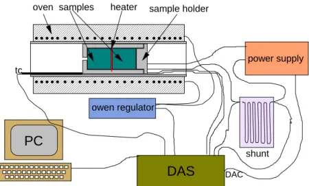
The experimental setup of the high temperature tests is shown in Fig. 1.

DAS

PC

owen regulator power supply tc shunt oven samples sample holder

DAC

heater

Fig. 1: Set up for the experiments at high temperature (DAS: data acquisition system; DAC: digital to analogue converter interface to drive the power supply)

The two identical samples are inserted in a special sample holder (see par. 3.1) together with the heather (par. 3.2), and the assemble is inserted into the oven, which is heated till to desired temperature (up to date 1200°C, future development 1500°C). The heater (electrically heated by a current flowing through it and fed by a power supply) behaves contemporarily as thermal source and a thermometer, as the platinum deposit behaves as a four wire resistance. The precise measurement of the current supplied is made inserting a 0.1 Ω shunt in series with the feeding circuit, The DAS (data acquisition system, a Keithley 2700 multimeter with 6.5 digit resolution) acquires voltages from the heater, the shunt and the thermocouple used to control the oven. A preliminary calibration is used to recognize the relation between the heater resistance and temperature. From the results of this calibration and the measurement of the voltage drop through the heater, the heater temperature is evaluated and used for the further data processing.

In the following the two innovative components of the system are described.

3.1. The heater

The heater is a platinum deposit on a ceramic thin substrate (yttria stabilized zirconia, 8YSZ), 0.1 mm thick, in square shape with 30 mm side. The material (generally used for fuel cell construction) is the thinnest ceramic substrate found and its thickness well represents the analytical solution, because a temperature variation along the thickness of the sample is unlikely.

The platinum coating is obtained by sputtering the platinum on the substrate surface. In order to respect the symmetry of the sample-heater system, both surfaces of the substrate are deposited with platinum, and also on one side of the substrate ridge in order to get short circuit between one surface and the opposite. The deposit has been studied in order to get the following features:

- resistance between 10 and 100 Ω in order to have good voltage resolution (and consequently temperature resolution) but within the range measurable with the DAS;

- good temperature distribution during heating, so the paths have been designed with the same wideness, trying to avoid too narrow direction changes;

(4)

Fig.2: design of the heater and its current path

With a 1 μm thickness of the platinum deposit and the shape designed and reported in Fig. 2, a total resistance of 60 Ω of the heater is calculated.

In order to verify if the heater presents good performances, an electromagnetic finite elements model has been built in order to simulate the electric resistance in the path, and hence the thermal power generation.

Fig. 3 reports the computed electric current density distribution in the central part of the heater, where the maximum disuniformity is expected. From this figure it is clearly possible to notice that only in the two points of direction inversion of the current flow a reduction of resistance, and hence an increasing of current, is expected. Even if this increase is very high (about 10 times the rest of the path), it is so concentrated in a very small region that its effect is practically undetectable. In fact a similar design had been already used for another heater, with a square winding of the electric path (see Fig. 4). The IR thermography detection of this heater (See Fig. 5) fed by an electric power does not reveal any meaningful temperature difference within the resolution of the IR camera (0.1 °C), even if in this heater many current inversion points are located.

(5)

Fig. 4 Heater with square winding of the electric path

Fig. 5 Thermography of the heater shown in fig. 4

3.2. The sample holder

The two identical samples and the heater must be located inside the furnace, in strict contact among them. Then the sample holder must assure this contact, must resist at high temperature, and must locate the two cylindrical samples and the square heater. The sample is positioned on the bottom of the holder, than the heater is put on it in its seat and then the other sample. A cap with a screwed side is used to keep all the items together and to impose the pressure to reduce the contact resistance. The material is a machinable ceramic (Aremco). Its look is shown in Fig. 6

(6)

Fig. 6 holder for sample in high temperature measurements

4. AMBIENT TEMPERAURE MEASUREMENTS

4.1. Experimental setup

Presently only tests at ambient temperature have been carried out, with a standard heater (Minco flat heater in capton with metallic deposit, in order to assess the experimental procedure and recognize the problems in the devices, experiment conduction and data processing. This heater was sandwiched between two samples of brick, and electric power supplied to it. So the experimental setup resulted the same as described before, except the oven and its control.

4.2. Results and data processing

( )

t s

( )

T C°

Fig. 7 non linear least square regression and residual analysis for test #1 ( )

t s

( )

(7)

Fig. 8 linear least square regression and residual analysis for test #2

The results of two different tests with samples taken from the same material (brick) and capton heaters are reported in Fig. 7 and 8, as temperature versus time.

From these data the presence of the thermal contact resistance is clearly noticeable, different in the two tests, and responsible of the high increasing of temperature in the first seconds of heating.

Fig. 7 and 8 reported also the non linear least square regression of the data of these two tests, together with the residuals analysis (difference between the calculated and experimental data, and showing the behaviour of data around the model). The best approximation of the unknown, their uncertainty and the prevision uncertainty of data are reported in Table 1. From the results the following remarks can be made:

- the analytical model well fits the data: an average difference of the data from the model of less than 0.1 °C is obtained

- thermophysical properties of brick are in agreement with reference data

- thermal contact resistance is different in the two tests, and in the first resulted 30% higher than in the second - at the beginning, during the initial quick heating, the maximum deviation between experimental and computed

data is present: this difference is likely due to the non perfect accordance between theory and experiments, i.e. the thermal contact resistance can be non uniform, and sample roughness can influence heat propagation in unpredictable way

(

_{W m}-1 _K-1

)

λ ⋅ ⋅ α

(

_m2⋅_s-1

)

(

_{W m}-2 _K-1

)

c h ⋅ ⋅ sT t

( )

°C Test #1 1.048 0.001±

(

6.76 0.02 10±

)

⋅ −7 90.97±0.57 _{3.61 10}⋅ −2 Test #2 1.0492 0.0003±

(

7.71 0.02 10±

)

⋅ −7 123.7 1.1± _{1.74 10}_⋅ −2

Table 1 – results of test #1 and #2

5. UNCERTAINTY ANALISYS

The uncertainty reported in table 1 is the propagation of the prevision uncertainty of data sT/t Being a result of the least square procedure, it can be seen as a type A uncertainty according to the definition of ISO GUM [9], because it is evaluated with a statistical method (least square regression). But this uncertainty represents only how experimental data are fitted by the analytical model, and by itself cannot be comprehensive of all the uncertainty causes.

Then type B uncertainty must be added. This can be due to:

- non perfect insulation of the sample from the environment: a deviation of the temperature values at longer times can take place, and influence the estimated parameters

- thermal capacity of the heater, at the moment evaluated only by reference data (in the future, when the final version of the heater will be available, its thermal capacity will be accurately determined)

( ) t s ( ) T C° ( ) t s ( ) T°C

(8)

- some amount of dependency of the two thermophysical parameters: thermal conductivity and thermal diffusivity. In fact the minimum sum of square of residual results little dependent on the variation of the two parameters. This corresponds to the so called “ill conditioned problem” [10], which sometimes make the least square procedure somehow faint.

On the contrary little uncertainty is attributed to propagation from other experimental conditions: supplied electric current, resistance variation of the heater during the test, length of the sample. So the sum in quadrature of these uncertainties to the others can be neglected.

As a conclusion a total uncertainty of ±5% (±1 σ) can be roughly estimated at the moment. A good assessment of the total uncertainty at high temperatures will be carried out with the analysis of all the uncertainty causes and tests with reference materials.

6. CONCLUSIONS

Contemporary measurement of thermal conductivity, thermal diffusivity and thermal contact resistance has been carried out with the flat plane source method. In order to perform this task, a data processing technique base upon non linear least square algorithm has been developed. This algorithm uses the analytical solution of the conduction heat transfer, and the lumped parameter equation for the heat stored in the heater and then transmitted to the sample through the thermal contact resistance. For high temperature tests (up to 1500°C) special devices (heater and sample holder) have been sized, designed and they are going to be realized in the next future. In the meantime assessment of the method has been carried out by means of a standard ambient temperature flat heater. Results show a good capacity of determining both thermophysical properties and contact resistance, even if the two properties evaluated are not completely independent on each other.

REFERENCES

[1] _{Silas E Gustafssonf, Ernest Karawackif and M Nazim Khan , “Transient hot-strip method for simultaneously} measuring thermal conductivity and thermal diffusivity of solids and fluids”, J. Phys. D: Appl. Phys., 12, 1411-1421 (1979).

[2]

Ramvir Singh, N S Saxena and D R Chaudhary, “Simultaneous measurement of thermal conductivity and thermal diffusivity of some building materials using the transient hot strip method” J. Phys. D: Appl. Phys. 18, 1-8 (1985) [3]_{J.P. Holman, Heat Transfer, Mac-Graw Hill, 48 (1981)}

[4]_{U. Hammerschmidt, “A New Pulse Hot Strip Sensor for Measuring Thermal Conductivity and Thermal Diffusivity of} Solids”, Int. J. Thermophys., 24, 675-682 (2003)

[5]_{S. E. Gustafssonf, E. Karawackif and M N. Khan, “Transient hot-strip method for simultaneously measuring thermal} conductivity and thermal diffusivity of solids and fluids”, J. Phys. D: Appl. Phys., 12, (1979).

[6]

M. Gustavsson, H. Wang, R. M. Trejo, E. Lara-Curzio, R. B. Dinwiddie, and S. E. Gustafsson

“On the Use of the Transient Hot-Strip Method for Measuring the Thermal Conductivity of High-Conducting Thin Bars”, Int. J. Thermophys., 27, 1816-1815 (2006)

[7]_{H.S. Carlslaw and J.C. Jaeger, Conduction of Heat in Solids, Clarendon Press, Oxford (1959)}

[8]_{S. Brandt, Statistical and Computational methods in Data Analysis, North Holland Publ., Amsterdam, (1970)} [9]

ISO/IEC Guide 98: “Guide to Expression of Uncertainty in Measurements” (1995)

[10]_{J.W. Beck and K.J. Arnold, Parameter Estimation, John Wiley and Sons, New York, (1977)}

APPENDIX

Analitical solution of the equation to be used as model in the least square regression

The geometry of the described experiments is sketched in Fig. A1. The differential equation is the usual Fourier equation

2 2 1 s s T T t x α ∂ ∂ = ∂ ∂ (A1)

(9)

where Ts is the temperature of the sample, an α the thermal diffusivity. The heat generation is assumed as a lumped

parameter first order differential equation in the Th , temperature of the heater:

(

)

h h c h s dT C h T T q dt + − =  (A2)

with Ch = mh cph the thermal capacity of the heater per unit area (mh the

mass per unit area of the heater, and cph its specific heat), and

2_{/ 2}

q=RI A, with R resistance of the heater and I the electric current flowing through it. The number 2 takes into account that the power is equally supplied to the two samples.

Eq. (A1) and (A2) are the two differential equations of a system whose unknowns are Ts and Th. The other boundary condition is the following:

0 s x L T x ₌ ∂ = ∂ (A3)

i.e. thermal insulation at the border of the sample, on the non heated side. This condition can be eventually modified if different

experimental setups are used The initial condition is

Ts = Th = T0 (A3)

with T0 the initial temperature of the test

The temperature differences from the beginning are defined:

0

s

T

s

T

ϑ = −

ϑ =_h T_h−T₀ (A4)

And the solution, computed in x=0, is given by [7], and is for ϑ_s

( )

₍

₎

(

)

2 2 2 / 2 1 1 3 6 / 2 1 1 2 6 1 n z t L n s n n z kZ qL k t Z k t Z k e k _L k P α α ϑ λ ∞ − =  ₊ ₊ ₋    = _ + − + + _ + __ +

∑

__  _(A5)

With the following positions

(

)

(

)

6 4 2 ₂ 2 ₁ 2 c n n n n h h L L Z k P z z Z Z kZ kZ k z C λ λ α = = = + + − + + (A6)

zn are the infinite solutions of the eigenvalue equation :

cotz z k

Z z

= − (A7)

which must be found numerically.

In order to have the analytical expression of ϑ_h which must be compared with the experimental data, the eq. A2 must be solved. According to the general rules of the linear differential equations, the equation A2 in the form

( )

1 h h h s c d q K t f t dt K h ϑ _ϑ  _ϑ  + = _ + _=    (A8) being K =h_c/C_h, must be solved first solving the associated homogeneous equation:

. . . . ₀ a h a h h h d K dt ϑ _ϑ + = (A9)

(a.h.= associated homogeneous), whose solution is

. . 1

a h Kt

h C e

ϑ = − (A10)

and than the particular solution. Taking into account that f(t) contains constant terms, one linear term in t and a sum of exponentials, the particular solution can be written as:

( )

. . 1 nt p s h n n t At B C e β ϑ ∞ − = = + +

∑

(A11)

{

h_c

{

hc samples _heater

Fig. A1: geometry of the analytical solution

(10)

where 2 n n z L α

β = . Naming A1, B1 and Cn1 the linear in t coefficient of f(t), the constant and the coefficient of the exponentials, i.e. 1 ₂ 1 c h h qL k A k _L C α λ   =  ₊    