technological externalities*
Giulio Bottazzi and Pietro Dindo
1. Introduction
The present contribution intends to pursue the analysis of the effects of the evolutionary metaphor (Dosi, 1988; Freeman, 1986; Nelson and Winter, 1982) when applied inside the domain of economic geography. in principle, the validity of the assumption of evolu-tionary economics is all but obvious and the question of whether economic interactions can be effectively thought of as an evolutionary process still open. With the clear risk of oversimplifying the matter, we could say that the notion of evolution immediately entails three consequences for the economic dynamics. First, it should move from simpler to more complex structures. Second, it should progressively eliminate less efficient struc-tures and promote the development of more efficient ones, irrespectively of the fact that this process of elimination and promotion might take place through a mechanism of adaptation by some of the economic actors or through an ‘adoptation’ by some of the markets and institutions (Alchian, 1950). Third, the progressive change or renewal of the different actors and rules should proceed in a jointly integrated way.
Obviously, the central question is not whether the characteristics described above can be considered to be present in economic systems, because they certainly are. The ques-tion is whether the evoluques-tionary accounting of their effects and causes allows for a deeper understanding and a more reliable modeling of economic interactions. in the end, one is interested to know if this accounting could help in the development of more effective poli-cies. in principle, however, the ideas of evolutionary economic thinking can be applied to the investigation of the different domains of economics also without providing a certain and indisputable answer to the previous question. Indeed, partly following, even if not subscribing to, the friedmanian idea that the effectiveness of a theoretical framework should be solely judged on its ability to reproduce and explain observed phenomena, one could simply start from the ‘evolutionary’ metaphor and see what consequences it brings to the design of economic models. As argued in Frenken and Boschma (2007), the devel-opment of an evolutionary approach to economic geography could suggest new ways of explaining the observed patterns that characterize the uneven spatial distribution of economic activities. In the spirit of the foregoing ‘minimalistic’ research agenda, we try to complement the bottom- up theorizing suggested there with a deeper understanding of the differences that an evolutionary inspired modeling is likely to produce with respect to more traditional approaches.
To be brought to its completion our exercise requires a twofold specification. First, we need to identify a simple formal model, based on clear assumptions, which can serve as a generic analytical framework. Second, we have to consider which hypotheses are to be put forward in order to imbue this model with the spirit of evolutionary economic geography. We address the first requirement by choosing, as a starting point, the simple
two- location and multi- firm model described in Krugman (1991). This model already encompasses the idea of increasing returns and of the relevance of feedback mechanisms in shaping the aggregate economic pattern. it is well rooted in the tradition of new eco-nomic geography and, as such, constitutes a perfect benchmark for our comparative exercise. Concerning the second requirement, in line with the discussion in Boschma and Frenken (2006) and Boschma and Martin (2007), and partly inspired by the critical survey in Martin (1999), we assume the following three aspects as baseline characters of our evolutionary modeling. first, the interaction between economic agents should take place not only through market mechanisms, but also through localized, idiosyncratic interactions. Second, the flow of time should be present in the model and the decisions of economic agents, together with their consequences, should be put in an explicit time dimension. Third, the heterogeneity of firms’ behavior should not be captured by a simple ‘noise’ term acting as a perturbation around a deterministic equilibrium. Rather, it should enter as an essential ingredient in the description of the model and in the deter-mination of the final aggregate outcome (Granovetter, 1978; Schelling, 1978).
more precisely, we take as a starting point the model introduced in forslid and Ottaviano (2003) and developed in Bottazzi and Dindo (2008). The latter extends Krugman (1991) by introducing a positive technological externality, assumed not trada-ble across locations, and by considering workers who are not mobile, which is equivalent to assuming that firms’ locational decisions and the reallocation of capital goods take place over a much shorter time scale than the one characterizing work- force flows. inside this simple economy, we consider a heterogeneous population of profit maximizing firms that independently choose where to locate their production. The model is characterized by a simple entry–exit process, and we consider a truly dynamic setting in which the locational decision of each firm is affected by the past decisions of others. As in Bottazzi et al. (2007), we assume that firms keep revising their decisions as new locational choices affect their profits. As we shall see, this updating choice process is able to generate a reinforcement mechanism similar to that described in Dosi and Kaniovski (1994).
The idea that localized externalities might explain agglomeration even in the absence of workers’ mobility, has been explored by several contributions inside new economic geography literature. For instance Krugman and Venables (1996) assume a vertically structured economy with localized input–output linkages, while martin and ottaviano (1999) consider location- specific R&D sectors that introduce different products in dif-ferent locations. Baldwin and Forslid (2000) consider geographical distributions of eco-nomic activities as driven by a growth process fueled by human capital accumulation and knowledge spillovers. A drawback of these works is that, in general, they derive equi-libria conditions without the complete and explicit characterization of firms’ profit func-tions. This specification becomes however necessary when one has to design the choice procedure of firms in a dynamic environment. In order to obtain explicit expression for the profit function, we take a simpler approach: we introduce technological externalities in the form of a baseline ‘cost sharing’ assumption, according to which fixed production costs are shared across all firms within a given location.
The cost sharing assumption makes the model in Bottazzi and Dindo (2008) particu-larly suitable for the present exercise because, while remaining simple and analytically tractable, it allows for a twofold dependence of firm profits on the activity of the other firms. Using the terminology of Scitovsky (1954), this dependence takes the form of both
a pecuniary externality and a technological externality. In this way, firms’ profits depend on the interplay of an indirect interaction mediated by the market, which corresponds to a pecuniary externality, and a localized direct interaction, which corresponds to a tech-nological externality. as it turns out, the former acts against the creation of production clusters while, by assumption, the latter promotes them.
Inside this framework, we analyze an explicit firms locational decision process. Our aim is to characterize the long run geographical distribution emerging from this process and relate it to the interplay of the two forms of externality. Since we explicitly intro-duce the time dimension in our analysis, we are also able to address history dependent phenomena. in particular, we are able to investigate how the initial state of the economy affects firms’ decisions and to show that, because of firms’ heterogeneity, when agglom-eration occurs it is characterized by a transient nature.
This chapter is organized as follows. in section 2 we briefly describe the model and its assumptions. in section 3 we study the static setting, and derive the geographical distribution when the model is solved by assuming instantaneous equilibrium between firms choices. Starting from the previously identified equilibria, section 4 introduces both heterogeneity in agents’ decisions and an explicit dynamics across time, discussing what kind of differences are observed with respect to the static case. finally section 5 summa-rizes our main findings and suggests some possible further developments.
2. The model
The following model is a simplification of that described in Bottazzi and Dindo (2008), where more details can be found. consider a two- location economy. in each location there are live I households.1 Each household is a ‘local’ worker, that is, he supplies labor to firms located where he resides, and a ‘global’ consumer, that is, he can buy goods produced in both locations and traded in a global market. The economy has two sectors: manufacturing and agriculture. in both sectors production is localized. The agricultural good is homogeneous, whereas the manufacturing good is made by differentiated prod-ucts. location l =1, 2 has nl manufacturing firms and the total number of firms is n1 + n2 = N. Without loss of generality, we assume that N is even. in order to consume manufac-turing goods produced in the location where they do not reside, consumers have to pay a transportation cost t [ (0, 1], which takes the form of an iceberg cost: for each unit of good shipped, only a fraction t arrives at the destination. This is equivalent to saying that consumers pay a price p/t for each unit of good they have to import. The higher the value of t, the lower the cost of transporting the goods. agricultural goods are traded at no costs. Agents’ consumption behavior is specified by the following
Assumption 1: each agent chooses among the agricultural goods and the N different manufacturing products so as to maximize the following utility function:
U 5 C12m
A CmM (24.1)
where the utility of bundle CM is of constant elasticity of substitution (CES) type,
CM5 a a i51,N cs21s i b s (s21) s .1 (24.2)
and each product ci is produced by a different firm i =1,. . .,N .
assumption 1 implies that the N products are substitutes and that s is the mutual elasticity of substitution (see Dixit and Stiglitz, 1977). The higher s, the more the prod-ucts are substitutes and the more impact on price differences consumers demand. Since, because of CES utility, agents value diversity, we have implicitly assumed that each firm produces a different product, so that N is both the number of manufacturing firms and the number of manufacturing products available for consumption.
The agricultural sector uses only labor as an input under constant returns to scale with unitary marginal costs. because of the large number of potential producers, 2I(1 − µ) at equilibrium, the agricultural market is perfectly competitive and the agricultural good is sold at its marginal cost.
Also manufacturing firms use only labor as input and their technologies are character-ized by a common, industry- specific, marginal cost and a local, location- specific, fixed cost. formally this leads to assumption 2.
Assumption 2: The labour vi that each firm i = 1, . . ., N needs to produce an amount yi of output is given by:
vi5byi1ali (24.3)
where marginal cost b is constant across firms and across locations and the fixed costs ali
depend on the location li occupied by firm i.
assumption 2 implies that we are in the presence of economies of scale, that is, an increase in output causes a decrease in each firm’s average costs. Firm i profit is given by:
pi = pi yi − wivi = yi( pi − wi b) − wiali, i = 1,. . ., N (24.4) where wi is firm i cost of labor.
Before looking for markets’ equilibria notice that, because of perfect competition and constant returns to scale in agricultural production, agricultural wages are equal to agricultural prices. moreover, because of zero transportation costs for the agricultural goods, agricultural prices, and thus wages, must be the same in both locations. Given that consumers are not mobile and the economy is at an equilibrium, it should also make no difference for a worker to work in the agricultural or in the manufacturing sector. As a result wages in the two sectors, and in the two locations, are equal. For this reason it is convenient to use wages to normalizes prices in the economy and set wi = 1 for all i.
In order to find equilibrium prices, quantities, profits in the manufacturing sector, and the resulting geographical distribution of firms, one should in principle analyze each of the N product markets. Nevertheless the problem can be simplified by considering only one representative market for each location. In fact, location by location, firms produce using the same technology, face the same demand (because of Assumption 1 all goods are substitutes), and the same labor supply. This implies that equilibrium prices, quantities and wages are the same for all the firms in a given location. We can thus consider only
two representative product markets, one for each location l, rather than the N distinct products.
We shall compute market equilibrium prices, quantities, and profits for each fixed distribution of firms, that is, fixing n1 and n2. First, exploiting the CES preference structure (24.2), which gives a constant elasticity of demand, and assuming that the market struc-ture is that of monopolistic competition, we derive firms’ pricing behavior. Then using households’ budget constraints we compute their total demand for the goods produced in each location, taking into account that all goods are substitutes and transportation costs impact the prices of foreign goods. Setting supply equal to demand we are able to determine equilibrium quantities and firms’ profits in each location as a function of n1 and n2. These expressions are used, in the next section, to assess firms’ geographical distribution.
Let us start from firms’ pricing behavior. Consistently with our assumptions, the market structure is that of monopolistic competition, that is, each firm maximizes its profits, setting its marginal revenue equal to its marginal costs, given market demand elasticity and irrespective of other firms’ behavior. Using profit function (24.4) and sub-stituting (24.3) while setting marginal profit to zero gives:
pla1 11e b 5b (24.5)
where e = ∂ log c/∂ log p is the demand elasticity. Given assumption 1, it holds that: e = −s
which together with (24.5) implies:
pl5b s
s 21 (24.6)
Since the price does not depend on the location index, local prices are equal and it holds
p1 = p2.
Denote the quantity demanded by an agent who reside in location l of a product pro-duced in location m as dlm. each demand can be determined as a function of prices and wages using the fact that relative demands under a CES utility satisfy:
d11 d12 5 a p2 p1tb s and d22 d21 5 a p1 p2tb s (24.7) while agents’ budget constraints give:
µ m 5n1d11p11n2d12 p2 t m 5n1d21 p1 t 1n2d22p2 (24.8) where, given the Cobb- Douglas formulation in (24.1), µ is the share of agents’ (unitary) income used to buy manufacturing goods. Solving for the demands, one finds:
d115 m n1p11n2ps1p12s2 ts21 d125 mts n1p12s1 ps21n1p2ts21 d225 m n1p12s1 ps2ts211n2p2 d215 mts n1p1ts211n2ps1p12s2 (24.9) Equating, location by location, firms’ supply and consumers’ demand, gives:
µ y15Id111 Id21 t y25Id221 Id12 t (24.10) where t discounts the demand of imported goods. Plugging (24.9) in (24.10) and using (24.6) one can solve for market equilibrium quantities:
µ y15 Im(s 21) bs a 1 n11n2ts21 1 t s21 n1ts211n2b y25 Im(s 21) bs a 1 n21n1ts21 1 t s21 n2ts211n1b (24.11)
Profits in each location can now be found using the latter expression together with (24.4) and (24.6). Introducing the fraction of firms in location 1, x = n1/N (so that n2 = (1 − x)N), and normalizing the level of wages to one, profits can be finally written as a function of x:
µ p1(x) 5 Im Nsa 1 x 1 (1 2 x)ts211 ts21 xts211 (1 2 x) b 2a1 p2(x) 5 Im Nsa 1 xts211 (1 2 x) 1 ts21 x 1 (1 2 x)ts21b 2 a2 (24.12)
Each location- specific profit function in (24.12) has a positive term proportional to the total demand for goods produced in that location and a negative term equal to the location- specific fixed costs. In turn, the total demand has a domestic component, the first term in the parentheses, and an import component, the second term in the parenthesis. Both components depend on firms’ geographical distribution and transportation costs. When the transportation cost is zero, t = 1, they are equal irrespective of firms’ distribu-tion. When the transportation cost increases, the domestic component increases, as local consumers substitute foreign goods with local ones. for the same reason, the export com-ponent decreases. For any given positive transportation cost, when local firm concentra-tion increases, the local component decreases as agents have more local goods to consume, all at the same price. in the same situation the export component increases, because foreign consumers have fewer local goods to consume and find it convenient to import more. The net effects of the transportation cost on the relative profits of the two locations are appraised in the next section. however, even without knowing this effect, it can immedi-ately be seen that market forces make the average profits independent of transportation costs. indeed one has the following:
Proposition 1 Consider an economy with two locations, l = 1, 2, and N firms, where
Assumptions 1–2 are valid. The average firms’ profit p does not depend on
transportation costs and is given by:
p 5 2Im
Ns 2xa12 (1 2 x)a2 (24.13)
Proof. See Appendix.
if now one assumes that a1 = a2, sine location- specific indexes have disappeared from any variable, only market forces are at work and our model becomes close to the one of Forslid and Ottaviano (2003). Following Bottazzi and Dindo (2008) we take a different route.
Before doing so, a last remark is necessary concerning the general equilibrium setting. In our framework, labor and goods markets are at equilibrium only when total firms’ profits are zero, and only provided that the demand for labor in both locations is not higher than I. Concerning the former condition, notice that profits are already zero for the com-petitive agricultural firms but not necessarily so for manufacturing firms. Nevertheless it is possible to set zero profit for the manufacturing sector, imposing a long- run equi-librium condition on the size of the economy. We shall do so in assumption 4 below. concerning the latter condition, one has that, because of labor market segmentation (no mobility), labor demand in both locations should be lower than I. Straightforward computations show that this amounts to imposing a restriction on the preferences for manufacturing goods, namely µ < s/(2s − 1), which we will assume to hold from now on.2 as a result, provided that preferences for manufacturing goods are not too strong and on imposing a long- run zero profit condition on the number of firms, prices and quantities as in (24.6) and (24.11) guarantee that both labor and good markets are at equilibrium.
Technological externalities
By retaining a dependency of the fixed cost a on the location index, we introduce a local-ized technological externality because of direct firms’ interaction, that is, not mediated by market forces (Scitovsky, 1954).
Assumption 3: ‘Cost sharing’ hypothesis. Firms’ fixed costs al decrease with the number of firms located in l according to:
a15 a
2x1, where xl 5 nl
N,l [ {0,1} (24.14)
assumption 3 represents a positive technological externality in the form of a baseline ‘cost sharing’: the larger the number of firms in one location, the lower the fixed costs these firms bear in the production activity. Since the fixed cost paid by firms in a given location decreases proportionally with the number of firms populating that location, the total fixed cost paid remains, location by location, constant. This effect can be thought of as an up- front cost paid to improve access to skilled labor, the more firms in one location the smaller each firm’s investment in training, or as a cost for services or infrastructure use, which is evenly shared among all the active firms in one location.
is that it doesn’t modify the total fixed costs paid by the industry. This has consequences on the computation of firms’ average profit.
Corollary 1 Consider an economy with two locations, l = 1, 2, and N firms, where
Assumptions 1–3 are valid. Total fixed costs in each location are equal to aN/2. The average firms’ profit p does not depend either on the distribution
of firms x or on transportation cost t and is given by:
p 52Im
Ns 2a (24.15)
Proof. See Appendix.
Before we start to look for geographical equilibria, that is, those spatial distributions of firms where they have no incentives to change location, notice that, without restrictions on the parameters’ values, there could exist economies characterized by negative profits. In this case, we would expect firms to exit the economy. On the other hand, if profits were positive we could expect firms to enter the economy. As we consider the number of firms N in the model as given, if there are no barriers to entry, it seems reasonable to set the number N to a level that implies zero profits. By force of Corollary 1 this can be done also without knowing the geographical equilibrium distribution. Indeed profits at a geographical equilibrium must be equal to average profits, and average profits (24.15), because of corollary 1, are independent on the geographical distribution x. moreover, as we have explained at the end of the previous subsection, zero total profits are needed in order to guarantee that all markets are at an equilibrium. All together, it is enough to have the following assumption.
Assumption 4: The number of firms N is such that profits at a geographical equilibrium are zero, that is:
N 52Im
sa (24.16)
even if, by construction, the previous assumption implies p = 0, outside the geograph-ical equilibrium profits can be both positive or negative so that their differential gives firms the incentive to relocate. Before moving to the analysis of these incentives and to the characterization of the geographical equilibria, it is useful to rewrite profits (24.12) incorporating assumptions 3–4: µ p1(x) 5a 2 a 1 x 1 (1 2 x)ts211 ts21 xts211 (1 2 x) b2 a 2x p2(x) 5a 2 a 1 xts211 (1 2 x) 1 ts21 x 1 (1 2 x)ts21b 2 a 2(1 2 x) (24.17) Given the firms’ production costs a, the products’ elasticity of substitution s and the transportation cost t, the distribution of firms between the two locations, x, determines, through (24.17), the levels of profit. Notice that in (24.17), differently from (24.12), both the demand driven term and the fixed cost term are functions of the geographi-cal distribution of firms. The first dependence is mediated by market forces (pecuniary
externality), whereas the second dependence is brought in by the ‘cost sharing’ hypoth-esis (technological externality).
3. Geographical equlibria
In this section we investigate the static geographical equilibria of the system, that is, those distributions of firms x such that, in the search for higher profits, each firm located in 1 has no incentives to move to 2 and vice versa. Geographical equilibria can be of two types: ‘border’ equilibria and ‘interior’ equilibria. A border equilibrium occurs when firms concentrate in one location, say 1, and profits in 1 are higher than profits in 2. As all the firms are in 1, no other firm can respond to this difference in profit opportunities. Candidates for border equilibria are x = 1, when all firms are in 1, and x = 0, when all firms are in 2. Conversely, an interior equilibrium occurs when firms distribute between the two locations, that is x [ (0, 1), profit levels are equal in both regions, and firms do not have any incentive to change their location. Using profits in (24.17) we will derive results for the existence and uniqueness of geographical equilibria, border and interior, for all the different parameterizations of the economy. This static3 analysis, which owes considerably to Bottazzi and Dindo (2008) where more details can be found, is useful to understand the interplay of pecuniary and technological externalities and constitutes a useful step for the development of the evolutionary dynamic analysis of the next section.
The respective role of each externality in determining profit differentials and thus the aggregate geographical equilibrium can be judged by looking at the shape of the profit functions and by keeping in mind that, because of transportation costs, local prices are lower than foreign prices, and thus local demand impacts firms’ level of output more than foreign demand. consider the pecuniary externality term alone, for example, set a = 0 in (24.17). For definiteness, consider profits in 1 (results for profits in 2 follow in the same way). For small x, that is, few firms in location 1 and many firms in location 2, each firm in 1 faces high local demand and low foreign demand. Because of the different impact of local and foreign demand, the level of output of firms in 1 is high and profits are high too. as x increases, the local demand for these firms decreases, so that profits decrease too. As the concentration of firms in 1 increases further, for a sufficiently large value of x, the demand coming from the consumers in 2, where very few firms are left, is more and more directed to 1 and the profits and the profits of firms located in 1 increase again. Profits are thus U- shaped, with p1(x)|a=0 first decreasing and then increasing in x. Since a firm makes the most profits when alone in one location, we have p1(x = 0)|a=0 > p1(x = 1)|a=0 so that the border distributions 0 and 1 are never an equilibrium. In fact, when all firm’s are located in one region it is always more profitable to move to the other region. If the transportation cost is increased (decreased), the variation in profits as a function of x is more (less) pronounced but the general shape of the profit function is pre-served. as a result, the overall agglomeration effect of the pecuniary externality is always ‘negative’, in the sense that it works against concentration of production.
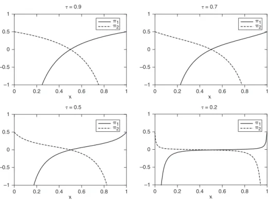
The above picture changes completely when one considers also the technological externality terms introduced by the ‘cost sharing’ assumption, that is, a > 0 in (24.17). The panels in figure 24.1 show graphs of p1(x) and p2(x) in this case. Profits are given by the superposition of a monotonically increasing technological externality to the U- shaped market- driven pecuniary externality term. With low transportation costs (high
t) the profit function is essentially determined by the ‘cost sharing’ term and is monot-onically increasing with decreasing marginal profits (upper panels of Figure 24.1). In this case, when firms’ concentration is low, firms do not benefit from the technological exter-nality and their profits are low too, but when concentration increases, profits increase monotonically as firms exploit the ‘cost sharing’ opportunity. The more the firms in one location, the lower the positive contribution of an extra firm locating there, so that the marginal profit decreases. With high transportation costs (low t) the shape of the profit function is still monotonic (bottom panels of Figure 24.1), but marginal profits are first decreasing and then increasing. With low firm concentration the technological externality dominates and marginal profits are decreasing. As the concentration increases, the posi-tive effect of the cost sharing is almost offset by the negaposi-tive market interaction, which acts as a constraint on the local demand faced by firms. In this case, even if profits are still increasing the marginal profit is almost zero. As the concentration of firms increases further, profits increase more steadily because low local demand is now compensated by the foreign demand, so that the contribution of the pecuniary externality is positive too. Judging from figure 24.1, irrespective of the transportation costs, the positive effect of technological externalities dominates the negative effect of pecuniary externalities: firms make most profits by agglomerating on one side and border distributions are always an equilibrium. This is formalized in Proposition 2.
–1 –0.5 0 0.5 1 0 0.2 0.4 0.6 0.8 1 x � = 0.9 �1 �2 –1 –0.5 0 0.5 1 0 0.2 0.4 0.6 0.8 1 � = 0.7 x �1 �2 –1 –0.5 0 0.5 1 0 0.2 0.4 0.6 0.8 1 x � = 0.5 �1 �2 –1 –0.5 0 0.5 1 0 0.2 0.4 0.6 0.8 1 x � = 0.2 �1 �2
Figure 24.1 Location profits (24.17) as a function of firms’ geographical distribution for
different values of the transportation cost t. Other parameters are s = 4 and a = 1
Proposition 2 Consider an economy with two locations, l = 1, 2 where Assumptions 1–4
are valid. Call x the fraction of firms located in 1. There always exist two,
and only two, geographical equilibria given by the border distribution x*151 and x*050. In particular, the unique distribution where profits are
equal, x* = 0.5, is never an equilibrium.
Proof. See Appendix.
According to the previous proposition, the distribution with half of the firms located in 1 and the other half located in 2, which is the unique case where p1 = p2, is never a geo-graphical equilibrium: even if profits are equal, incentives are such that firms move away and agglomerate. Only when all firms are located either in 1 or 2 are there no incentives to change location.
Notice that, even if transportation costs do affect the shape of each location’s profit function, they have no impact in characterizing the geographical equilibria of the economy. conversely, as we shall see in the following section, transportation costs play a major role in shaping the results of the evolutionary model, even in the long run.
4. Evolutionary firm dynamics
in the previous section we have shown that, when the technological externality term is introduced, firms agglomerate in one of the two locations, irrespective of transporta-tion costs t or the relevance of technological spillover as dependent on a. This abrupt behavior would prescribe that any sector in which even a minimal level of localized pecuniary externalities operate should display a so- called core–periphery structure. This is clearly at odds with empirical observations. notice that this conclusion would remain a fortiori valid if instead we had considered workers’ mobility with endogenous wage setting, thus introducing a feedback effect that reduces (or inverts) the push of pecuni-ary externalities towards a symmetric geographical distribution. This effect ultimately reinforces the conclusion that in the presence of technological spillovers only a core– periphery structure represents an equilibrium. We end up in the uncomfortable situation of having a single possible equilibrium, implying the impossibility of performing an empirical analysis or deriving policy implications. a possible way out from this impasse, as we will show, is to extend the notion of geographical equilibrium to include an explicit dynamics describing firms’ locational decisions. The foregoing analysis is, indeed, essen-tially static and thus silent on the results of firms’ interactions out of equilibrium. As a consequence, it is not clear what happens when the initial concentration of firms is not at an equilibrium level; in particular, whether one should expect firms to agglomerate in location 1 or in location 2.
in this section we extend our analysis by introducing heterogeneity in preferences at the single firm level and by explicitly modeling firms’ decisions in time, that is, by allow-ing for a dynamic location- specific mechanism. Suppose that the individual utility of firm
i derived from locating in li can be written as: pi = pl
i + ei,li (24.18)
where pli are as in (24.17) and ei,li represents an idiosyncratic profit component intended
different fixed costs or individual preferences for one particular location, because of, for instance, existing social linkages. At every time step a firm is randomly chosen to exit the economy. At the same time a new firm enters and chooses whether to be located in 1 or in 2 by comparing the individual utilities in (24.18). As long as the distribution of ei,l across firms is well behaved (see Bottazzi and Secchi, 2007; Bottazzi et al., 2008, for details) the resulting probability of choosing l is given by:
probl5 e pl
ep11ep2, l [ {1,2} (24.19)
The fact that the locational choice is probabilistic derives from the assumption that the new entrant possesses preferences, or faces costs, that are not fixed, but contain an indi-vidual component that is randomly extracted from a given distribution.
When the probability of choosing location l is given by (24.19), Bottazzi and Secchi (2007) show that, if the exponentials of profits are linearly changing in the number of firms, it is possible to compute the long- run stationary distribution of the entry–exit process. Thus, to exploit this result we need a linearized version of the exponential profit functions. We can naturally obtain it as the deviation from the middle point x* = 0.5, that is, the unique point where profits are equal.
Proposition 3 Consider an economy with two locations, l = 1, 2, where Assumptions 1–4
are valid. Denote the linearization of location l exponential profits around
x* =0.5 as cl, and the number of firms in location l as n
l. Linearized
expo-nential profits are given by:
cl = a + bnl, l =1, 2 (24.20)
where:
a 51 2 (1 1 t4ats21s21)2
b 5 4a2sts21
Im(1 1 ts21)2 (24.21)
Proof. See Appendix.
We shall call the term a in (24.21) the ‘intrinsic profit’. This is the part of the common profit that is entirely dependent on exogenously given characteristics of the location. conversely, the coefficient b in (24.21) captures the marginal contribution of a firm to the profit level of the location in which it resides. We shall call it the ‘marginal profit’.4 in our case, this coefficient captures the total effect of pecuniary and technological externalities. because of the leading effect of the latter it is always positive but, because of the presence of market mediated interactions, it is dependent on transportation costs. Specifically, the marginal profit is increasing with the value of t. When transportation costs are high (low t) each firm’s marginal contribution to the location profit is small, whereas when transportation costs are low (high t ) the marginal contribution is large.
Given the linearization in (24.20), the following proposition characterizes the long- run geographical equilibrium distribution.
Proposition 4 Consider an economy with two locations, l =1, 2, where Assumptions 1–4
are valid. The economy is populated by N firms, distributed according to n = (n1, n2). At the beginning of each period of time a firm is randomly selected,
with equal probability over the entire population, to exit the economy. Let
m [{1, 2} be the location affected by this exit. After exit takes place, a
new firm enters the economy and, conditional on the exit that occurred in m, has a probability:
probl5
a 1 b(n12dl,m) 2a 1 bN
of choosing location l, where a and be are given by (24.1). This process admits a unique
stationary distribution: p(n) 5N!C(N, a, b) Z(N, a, b) q 2 l51 1 nl! nl(a, b) (24.22) where: C(N, a, b) 5 2a 1 a1 2Nb1 bN (24.23) n(a, b) 5 e q n h51[a 1 b(h 2 1) ] n . 0 1 n 50 (24.24)
and Z(N, a, b) is a normalization factor which depends only on the total number of firms N,
and the coefficients a and b.
Proof. See Propositions 3.1–3.4 of Bottazzi and Secchi (2007).
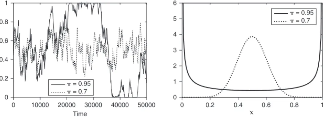
figure 24.2 shows results from a simulation of the entry–exit process for two different values of the transportation cost t. The left panel shows 50,000 iterations of the process,
0 0.2 0.4 0.6 0.8 1 0 10000 20000 30000 40000 50000 Time 0 1 2 3 4 5 6 0 0.2 0.4 0.6 0.8 1 x � = 0.95 � = 0.7 � = 0.95 � = 0.7
Figure 24.2 Entry–exit process for different values of the transportation costs. Left
panel: 50,000 simulations of the entry–exit process for different values of the transportation cost t . Right panel: Long- run stationary distribution of the
entry–exit process simulated in the left panel. In both panels the parameters
whereas the right panel plots the corresponding long- run distributions as characterized by proposition 4.
With low transportation costs (t = 0.95) the long- run distribution is clustered around the two extreme values, x = 0 and x = 1, confirming the prediction of the static analysis. However, the simulation of the entry–exit process (left panel of Figure 24.2) shows that agglomeration is only a meta- stable state. one location can become much larger than the other for several time steps, like location 2 which, in the simulation shown, attracts almost all firms in the periods between 2000 and 3500, but at some point the cluster abruptly disappears and the other location can take over. This behavior is well in accord-ance with the bimodal nature of the equilibrium distribution (see right panel of Figure 24.2). In fact, the equilibrium distribution represents the unconditional probability of finding the system in a give state. This probability can thus be very different from the frequency with which this particular state is observed over a finite time window.
Conversely, for higher transportation costs (t =0.7), agglomeration is ‘almost’ never observed: firms spatial distribution is now fluctuating around x* =0.5 (see left panel of Figure 24.2). Even if the static analysis predicts agglomeration, the equilibrium distribu-tion of the stochastic system, reported in the right panel of figure 24.2, shows that the most likely geographical distribution has an equal number of firms per location, irre-spective of the fact that the point x* = 0.5 is never a static geographical equilibrium. In general one has the following:
Proposition 5 Consider the entry and exit process described in Proposition 4. When the
marginal profit is bigger than the intrinsic profit, b > a, the stationary dis-tribution (24.22) is bimodal with modes in x = 0 and x = 1; when b < a the
stationary distribution is unimodal with mode in x = 0.5; and when a = b
the stationary distribution is uniform.
Proof. See Appendix.
Given our dynamic locational decision process, the previous proposition clarifies that the shape of the geographical equilibrium distribution does ultimately depend on the relative size of the marginal profit b and the intrinsic profit a. When marginal profits are bigger than intrinsic profits the distribution has mass on the borders of the [0, 1] interval. When marginal profits are lower than intrinsic profits the distribution has higher mass in the middle of this interval, and when they are equal every value of the geographical distribution is as likely.
rewriting the relation b _ a in Proposition 5 using the definitions of a and b in (24.21), it is straightforward to derive the conditions for the unimodality or bimodality of (24.22) in terms of the values of t, I, µ, and a:
4aa1 1asIm b _ (1 1 t s21)2 ts21
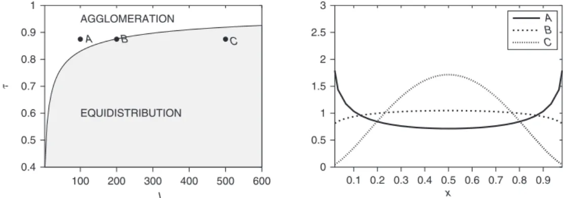
The left panels of Figures 24.3 and 24.4 have been obtained using the latter inequality: they show which distributional shape is observed in the different regions of the plane (I, t) and (a, t) respectively. In the white area agglomeration is most likely (bimodal distribution), whereas in the dark area equidistribution is most likely (unimodal distri-bution). In the right panels the stationary distributions computed at the corresponding
points A, B, and C are shown. In both figures these points have been obtained by keeping t fixed.
The right panel of figure 24.3 shows that moving from small to large values of I while keeping t fixed, the long- run distribution changes from bimodal to unimodal. This is because an increase in the number of residents I leads to a decrease in the marginal profit
b (see 24.21). In fact, as a result of Assumption 4, the more residents there are, the more firms there are and the smaller the contribution of each firm’s locational decision to the profits of other firms, that is, the smaller the marginal profit. Changing I corresponds to
0.4 0.5 0.6 0.7 0.8 0.9 1 100 200 300 400 500 600 � I AGGLOMERATION EQUIDISTRIBUTION A B C 0 0.5 1 1.5 2 2.5 3 0.1 0.2 0.3 0.4 0.5 0.6 0.7 0.8 0.9 x A B C 0 0.2 0.4 0.6 0.8 1 0.9 0.95 1 1.05 1.1 1.15 1.2 1.25 1.3 1.35 1.4 � � AGGLOMERATION EQUIDISTRIBUTION C B A 0 1 2 3 4 5 0.1 0.2 0.3 0.4 0.5 0.6 0.7 0.8 0.9 x A B C
Figure 24.3 Entry–exit process for different values of the number of residents I.
Left panel: A portion of the space (I, t) has been divided into the ‘agglomeration’ area (white) and the ‘equidistribution’ area (shaded) according to Proposition 5. Right panel: Stationary geographical
distributions computed at the points A, B, and C. Other parameters are a = 1, µ =0.5 and s = 4, whereas N is fixed by Assumption 4
Figure 24.4 Entry–exit process for different values of the fixed costs a. Left panel: A
portion of the space (a, t) has been divided into the ‘agglomeration’ area (white) and the ‘equidistribution’ area (shaded) according to Proposition 5. Right panel: Stationary geographical distributions computed at the points
A, B, and C. Other parameters are I = 400, µ =0.5 and s = 4 whereas N is
a sort of ‘size’ effect: increasing the size of the economy lowers the externalities so that, because of the entry–exit process, the likelihood of observing agglomeration is lowered.
The right panel of figure 24.4 shows that, keeping t fixed, an increase in the fixed cost parameter a leads, in general, to more agglomerated economies. it is so because an increase in a decreases the intrinsic profit a while increasing the marginal profit b. more precisely, a determines the scale of the profit differentials. Indeed, on the one hand, the difference between the maximum and the minimum profit is proportional to a and, on the other hand, because of assumption 4, the higher a the lower N, so that a bigger profit difference is caused by a lower number of firms. As a result, increasing fixed costs decreases the profit each firm earns irrespective of the presence of other firms, and increases the effect of each locational choice on the profits of others. Both effects go in the direction of increasing the likelihood of agglomeration. This is a sort of ‘scale’ effect where increasing the scale of profits increases the likelihood of agglomeration.
Concerning the effect of the transportation cost on the shape of the equilibrium dis-tribution, notice that the expression ts−1/(1 + ts−1)2, which appears in (24.21) for both a and b, but with a different sign, is an increasing function of t. Thus, increasing the value of t leads to an increase in the marginal profit b and a decrease in the intrinsic profit a. This means that low transportation costs, that is, high values of t , favor agglomeration, while high transportation costs favor equidistribution. Indeed, when transportation costs are low, the pecuniary externality is relatively weak and the technological exter-nality relatively strong. in terms of the entry–exit process, the choices of a relocate its activity has an high impact on the level of profits. Consequently, it is likely to trigger other relocations and, eventually, a strong agglomeration is observed. conversely, when transportation costs are high, the pecuniary and technological externalities almost offset each other. This implies that marginal profits are small and intrinsic profits dominate, so that each locational choice has a very small impact on the general level of profits. The attracting force of each location does not depend on the externality term and, given the symmetry of the two locations, equidistribution is likely to be observed.
5. Conclusion
We have analyzed a model of firms’ location in geographical space where firms interact both indirectly, through market interactions, and directly, through technological exter-nalities, and where workers are not mobile. in this simple framework we have briefly discussed the general equilibrium static case, identifying the possible geographical equilibria, that is, the spatial distributions in which firms do not have any incentive to relocate their activities. We have showed that in this case the ‘cost sharing’ assumption implies long- run agglomeration, irrespective of the number of consumers, their prefer-ences, and transportation costs. Then we have extended the analysis to include heteroge-neity in firms’ preferences and an explicit time dynamics in their choices, thus obtaining a stochastic model of firms’ dynamics. We have been able to characterize the long- run geographical distribution of the process for different specifications of the economy. This analysis has revealed that, contrary to the static equilibrium analysis, when an explicit entry–exit dynamics is assumed to characterize the locational decision of firms, the economy can evolve towards two different long- run scenarios. In the first scenario, where externalities are stronger than intrinsic location profits, which typically occurs for low transportation costs, the long- run geographical distribution is bimodal with modes
at the extremal outcomes x = 0 and x = 1. Agglomeration is thus the most likely event but, as simulations show, this does not mean that once agglomeration on one side has been achieved, the situation is stable. In fact, turning points exist where the mass of firms moves from one location to the other. in the second scenario the long- run geographi-cal distribution has a unique mode. In this case, the most likely occurrence is having half of the firms located in one region and the other half in the other region. However, because of the stochastic nature of the process, fluctuations around this average level are present. This scenario is typically associated with high transportation costs, and occurs, in general, when the effect of externalities is weak with respect to the intrinsic profit levels of each location.
Summarizing, the main contribution of the foregoing analysis is to show how firms’ heterogeneity and an individual choice process act as brakes or constraints on firms’ agglomeration, even when strong incentives to locate in already populous locations exist. moreover, having introduced an explicit time dimension, we have given history a role. Indeed the time dimension matters in two respects: first, the initial distribution of activities across two locations does influence the subsequent observed distributions and, second, when agglomeration is observed, because of stochastic fluctuations, it is only a metastable phenomenon. That is, by waiting long enough, the cluster eventually disap-pears, just to be recreated soon after, with probability 1/2, in the other location.
Our model can be extended in several directions. First of all, the ‘cost sharing’ assump-tion, while useful, is admittedly ad hoc. more careful modeling is probably needed. The effort should not be restricted to the notion of technological and/or knowledge spillover, which might even be characterized by a pecuniary nature, see, for example, antonelli (Chapter 7, this volume), but could encompass also other, possibly negative, sources of interactions that are not market mediated, like pollution and/or congestion effects. a second extension of the model would be to generalize consumers’ behavior along the same lines we followed to describe firms’ behavior. Whereas in the present version of the model consumers are homogeneous and maximize the same CES utility function, it would be interesting to assume that consumers are heterogeneous and to explicitly model their consumption decision in time. in that case, changing the size of the economy would imply, because of varying idiosyncrasies in consumers’ demand, a change in the amplitude of profit fluctuations. This, in turn, would impact the likelihood of observing agglomerated outcomes, probably reducing it.
in any case, we are aware that the ultimate test will be to confront our model with real data. an interesting aspect of the discrete choice model we implemented is that it leads quite easily to empirical applications. An exercise in this direction has already been performed in Bottazzi et al. (2008), where the parameters characterizing the geographi-cal equilibrium distribution have been estimated in several sectors of the Italian manu-facturing industry. The present work moves in the direction of developing a theoretical framework able to provide deeper and more informative economic interpretations of these econometric exercises.
Notes
* Thanks to the participants to the DIMETIC Summer School ‘Geography of Innovation and Growth’, Pecs, Hungary; the First DIME Scientific Conference, Strasbourg, France; and seminars given at the Universit`a degli Studi di Napoli ‘Parthenope’ and at the Scuola Superiore S’Anna, Pisa, Italy. The research that has
led to this work has been supported by the EU FP6 STREP Project CO3 Common Complex Collective Phenomena in Statistical Mechanics, Society, Economics, and Biology and by the European Union NoE dime. all usual disclaimers apply.
1. The generalization to different numbers of agents in each location will be considered in future work. Preliminary analysis shows that it doesn’t significantly modify the results.
2. This is the same condition found in Forslid and Ottaviano (2003). See Bottazzi and Dindo (2008) for more details.
3. Technically our geographical equilibrium corresponds to a Nash equilibrium in pure strategies of the one shot game where each firm in a group of N has to choose whether to be located in 1 or in 2 and payoffs are given by profits.
4. In the terminology of Bottazzi and Secchi (2007) the intrinsic profit corresponds to the location’s ‘intrinsic attractiveness’, whereas the marginal profit is the ‘social externality’.
References
Alchian, A. (1950), ‘Uncertainty, evolution, and economic theory’, The Journal of Political Economy, 58, 211–21.
Baldwin, R. and R. Forslid (2000), ‘The core–periphery model and endogenous growth: stabilizing and desta-bilizing integration’, Economica, 67, 307–24.
Boschma, R. and K. Frenken (2006), ‘Why is economic geography not an evolutionary science? Towards an evolutionary economic geography’, Journal of Economic Geography, 6, 273–302.
Boschma, R. and R. Martin (2007), ‘Editorial: Constructing an evolutionary economic geography’, Journal of
Economic Geography, 7, 537–48.
Bottazzi, G., G. Dosi, G. Fagiolo and A. Secchi (2007), ‘Modeling industrial evolution in geographical space’,
Journal of Economic Geography, 7, 651–72.
Bottazzi, G., G. Dosi, G. Fagiolo and A. Secchi (2008), ‘Sectoral and geographical specificities in the spatial structure of economic activities’, Structural Change and Economic Dynamics, 19, 189–2002.
Bottazzi, G. and A. Secchi (2007), ‘Repeated choices under dynamic externalities’, LEM Working Paper 2007–08, Sant’Anna School for Advanced Studies, Pisa.
Bottazzi, M. and P. Dindo (2008), ‘Localized technological externalities and the geographical distribution of firms’, LEM Working Paper 2008–11, Sant’Anna School of Advanced Studies.
Dixit, A. and J. Stiglitz (1977), ‘Monopolistic competition and optimun product diversity’, American Economic
Review, 67 (3), 297–308.
Dosi, G. (1988), ‘Sources, procedures, and microeconomic effects of innovation’, Journal of Economic
Literature, 26, 1120–71.
Dosi, G. and Y. Kaniovski (1994), ‘On “badly behaved” dynamics’, Journal of Evolutionary Economics, 4, 93–123.
Forslid, R. and G. Ottaviano (2003), ‘An analytically solvable core–periphery model’, Journal of Economic
Geography, 3, 229–40.
Freeman, C. (1986), The Economics of Industrial Innovation, 2nd edn, cambridge, ma: miT press.
Frenken, K. R. Boschma (2007), ‘A theoretical framework for evolutionary economic geography: industrial dynamics and urban growth as branching process’, Journal of Economic Geography, 7, 635–49.
Granovetter, M. (1978), ‘Threshold models of collective behavior’, The American Journal of Sociology, 83 (6), 1420–43.
Krugman, P. (1991), ‘Increasing returns and economic geography’, The Journal of Political Economy, 99, 483–99.
Krugman, P. and A. Venables (1996), ‘Globalization and the inequlity of nations’, Quarterly Journal of economics, 110, 857–80.
Martin, P. and G. Ottaviano (1999), ‘Growing locations: industry locations in a model of endogenous growth’, european economic review, 43, 281–302.
Martin, R. (1999), ‘The new “geographical turn” in economics: some critical reflections’, Cambridge Journal
of Economics, 23, 65–91.
Nelson, R. and S. Winter (1982), An Evolutionary Theory of Economic Change, cambridge, ma: harvard university press.
Schelling, T.C. (1978), Micromotives and Macrobehavior, new york: W.W. norton.
Appendix
Proof of Proposition 1 and Corollary 1
Average profits follow in a straightforward way by computing p 5 xp1(x) 1 (1 2 x)p2(x) with p1(x) and p2(x) as in (24.12) and in (24.17). Total costs in each location are equal because (24.14) implies: a i51,n1 ai5 a j51,n2 aj5 Na 2 Proof of Proposition 2
First, the unique distribution of firms where profits are equal is x = 0.5. Indeed taking profits as in (24.17), setting p1(x) equal to p2(x), gives a first order equation in x whose unique solution is x = 0.5.
Geographical equilibria are pure strategy Nash equilibria (PSNE) of the one stage game where each firm in a group of N (N even), has to choose to be located in l =1 or l = 2 and profits are given by (24.17). Denote the firm i = 1, . . ., N strategy as si. firm i can choose to locate either in 1, si = 1, or in 2, si = 0. The strategy space has thus 2N elements. A strategy profile will be denoted as s while s−i will denote the strategy profile of the N − 1 firms apart from i. Define also:
x(s) 5 ai51,. . .,N si
N
To complete the formalization of the game we have to specify each firm payoff for any strategy profile s. When si = 1, firm i payoff pi is given by:
pi(1, s2i) ; p1(x(s))
where p1(x) is as in (24.17) and x(s) is defined above. When si = 0, firm i payoff is: pi(0, s2i) ; p2(x(s))
where p2(x) is again from (24.17). To give an example, if all firms choose location l = 1, so that x = 1, one has pi5p1(1) for all i = 1,. . ., N. If, instead, half of the firms are located in l = 1 and the other half in l = 2, so that x =0.5, one has pi5p1(0.5) if si = 1 and pi5p2(0.5) otherwise. A strategy profile s* is a PSNE if and only if:
pi(s*i, s*2i) $ pi(si, s*2i) for all si = 0, 1, i = 1,. . ., N (24A.1) The only candidates to be PSNE are those strategy profiles s for which x(s) [ {0, 1, 0.5}. We start by showing that every s* such that x(s*) = 1 or x(s*) = 0 is a PSNE profile. From (24.17) it holds that p1(1) . p2(x) for all x [ (0, 1) and p2(0) . p1(x) for all
x [ (0,1), so that (24A.1) is satisfied. Then consider a strategy profile s* such that
x(s*) 5 x* 5 0.5. Given (24A.1), it is a PSNE if and only if: p1(0.5) $ p2a0.5 2 1
p2(0.5) $ p1a0.5 1 1
Nb4i 51, . . ., N (24A.3)
Since the two locations are identical and x is the share of firms choosing location 1, by symmetry it holds that p1(x) 5 p2(1 2 x). using this relation we can rewrite both (24A.2) and (24A.3) as:
p1(0.5) $ p1a0.5 1 1
Nb4i 51, . . ., N
The latter is satisfied if and only if the function p1(x) is not increasing at x = 0.5. Direct computation of dp1(x)/dx0x50.5 (see the following proofs for the explicit expression) shows that this is never the case, implying that the symmetric distribution is never a PSNE.
Proof of Proposition 4
Consider the Taylor expansion up to the first order of each term in (24.17) as a function of z = x − 0.5:
p1(z) 5 p1(0.5) 1 z(2)la2aa1 2 ts21 1 1 ts21b
2
22ab 1 O(z2), l 5 1, 2
using the expressions above to linearize exppl in (24.19), and writing them in terms of the number of firms nl, l =1, 2 we obtain the expressions of the linearized exponential payoff cl, c151 2 2aa(1 2 t s21)2 (1 1 ts21)221b a n1 N2 1 2b c251 1 2aa(1 2 t s21)2 (1 1 ts21)221b a 1 22 n2 Nb
This shows that a and b are given by:
a 51 1 aa(1 2 t(1 1 ts21s21))2221b
b 5 22a N a
(1 2 ts21)2 (1 1 ts21)221b which, using assumption 4 to eliminate N, correspond to (24.21).
Proof of Proposition 5
From (24.22) it follows that the distribution is symmetric around N/2, that is p(N/2 1 n) 5 p(N/2 2 n) for every n 5 0, . . ., N/2. Consequently it suffices to analyse the set {0,. . .,N/2}.
When a = b, qn(a, b) reduces to n!. As a result the probability density becomes: p(n) 5 N!C(N, a, b)
so that the distribution is uniform. The rest of the lemma will be proved by induction. first consider: p(0) _ p(1) N!C(N, a, b) Z(N, a, b) 1
N!qN(a, b) _ N!C(NZ(N, a, b), a, b) (N 2 1)!1 q1(a, b)qN21(a, b) a(a 1 b). . .(a 1 b(N 2 1)) _ Na2(a 1 b). . .(a 1 b(N 2 2))
b _ a (24A.4) Second consider: p(n) _ p(n 1 1) N!C(N, a, b) Z(N, a, b) 1 n!(N 2 n)!qn(a, b)qN2n(a, b) _ N!C(N, a, b) Z(N, a, b) 1 (n 1 1)!(N 2 n 2 1)!qn11(a, b)qN2n21(a, b) (n 1 1)a(a 1 b). . .(a 1 b(n 2 1))a(a 1 b). . .(a 1 b(N 2 n 2 1))
_ (n 1 1)a(a 1 b). . .(a 1 bn)a(a 1 b). . .(a 1 b(N 2 n 2 2))
b(N 22n 2 1) _ B(N 2 2n 2 1)
b _ a (24A.5)
where the last step requires n # N/2 2 1, which is our case. from 24a.4 and 24a.5 it follows that when b > a the maximum is in p(0) (and by symmetry in p(N)), whereas, when b < a, the maximum is in p(N/2).