Characterisation and calibration of optical counters for airborne particulate matter

(1)

ALMA MATER STUDIORUM · UNIVERSITÀ DI BOLOGNA

FACOLTÀ DI SCIENZE MATEMATICHE, FISICHE E NATURALI Corso di Laurea Magistrale in Fisica del Sistema Terra

Characterisation and calibration of

optical counters for airborne particulate

matter

Relatore: Presentata da: Prof. Vincenzo Levizzani Agostino Rappazzo

Co-relatori:

Dott. Franco Belosi Dott. Fabrizio Ravegnani

I Sessione

(2)

(3)

III

Sommario

Con il termine aerosol, o particolato ambientale (PM), si definisce una sospensione colloidale di particelle solide o liquide in aria. Gli aerosol sono parte integrante dell’atmosfera, hanno un ruolo importante in diversi processi atmosferici e influenzano il clima terrestre e la salute umana con effetti di diminuzione dell’aspettativa di vita. E’ pertanto di primaria importanza il loro monitoraggio in tempo reale in termini di concentrazione e distribuzione dimensionale.

I contatori ottici di particolato ambientale (OPC) sono largamente usati in monitoraggi in ambienti sia outdoor che indoor. Si basano sullo scattering di un fascio luminoso collimato per classificare le particelle e fornire concentrazioni in numero di aerosol in tempo reale. Misurano dimensionalmente particelle di dimensioni comprese tra 0.3 e 20 μm e concentrazioni in numero fino a 107_{# L}-1_{. Recenti progressi nella tecnica hanno} permesso la commercializzazione di OPC portatili di dimensione e costo ridotti; tali strumenti sono adatti per valutazioni di esposizione personale al particolato ambientale, nonché per implementare reti di monitoraggio diffuse (smart cities).

Gli OPC richiedono calibrazioni frequenti, che vengono solitamente effettuate producendo aerosol di dimensione controllata e testando la risposta dell’OPC da calibrare con uno strumento di riferimento (ad esempio, uno strumento già calibrato) o con valori assoluti di concentrazione ottenuti tramite osservazione diretta di particelle tramite un microscopio elettronico a scansione (SEM).

Gli obiettivi di questo lavoro sono:

1) la caratterizzazione delle prestazioni di un OPC di nuova concezione (CompactOPC N1, prodotto da Alphasense; in seguito COPC) confrontando l’output con quello di un OPC standard commerciale (Portable Laser Aerosolspectrometer Dust Monitor Model 1.108, prodotto da GRIMM AEROSOL Technik GmbH & Co.; in seguito GRM);

2) la realizzazione di un banco di prova per la calibrazione di un OPC utilizzato in camere bianche e ambienti sanitari (Laser Particle Sensor mod. 3715-00, prodotto da Kanomax; in seguito LPS).

(4)

IV

La ditta Pollution Clean Air Systems S.p.A (Budrio, BO), il distributore italiano del LPS, è interessata a effettuare la calibrazione di tale OPC per i propri clienti, dal momento che tale attività non viene effettuata in Italia. Pertanto, la ditta ha manifestato interesse per i risultati di questo lavoro per migliorare potenzialmente il proprio servizio ai clienti. Le prove sono state effettuate con aerosol indoor e con particelle monodisperse di latex polistirene (PSL) di dimensioni differenti campionando in parallelo con i diversi OPC e su filtro per osservazioni al SEM. In questo modo si è ottenuto un valore assoluto di riferimento per la concentrazione di aerosol. I risultati indicano un buon accordo tra il GRM e i dati ottenuti dalle analisi al SEM, confermando pertanto una buona affidabilità del setup sperimentale e del GRM. Dai risultati si evince anche che se munito di una pompa, invece che di una ventola come nella configurazione standard, il COPC fornisce le migliori prestazioni.

Per il secondo scopo, il LPS è stato calibrato generando aerosol monodisperso e confrontando l’output con quello di un altro LPS calibrato di recente.

Il lavoro sperimentale relativo a questa tesi è stato effettuato presso il Laboratorio di Aerosol e Fisica delle Nubi dell’Istituto di Scienze dell’Atmosfera e del Clima (ISAC) del Consiglio Nazionale delle Ricerche (CNR) a Bologna.

(5)

V

Abstract

The term aerosol, or particulate matter (PM), defines a colloidal mixture where liquid and solid particles are suspended in the air. Aerosols are therefore an integral part of the atmosphere, play an important role in most of the atmospheric processes and affect the Earth’s climate and human health with decreases in life expectancy. Therefore, it is of primary importance to monitor aerosol concentrations and size distributions on a real-time basis.

Optical Particle Counters (OPCs) are widely used for monitoring outdoor and indoor ambient air. They rely upon light scattering to classify aerosol particles and return particle number concentrations on a real-time basis. They can measure particle sizes from 0.3 up to 20 μm and particle number concentrations up to 107_{# L}-1_{. Recent progresses in} technique have allowed the commercialisation of smaller, cheaper and portable OPCs, which are well suited for personal exposure assessment to airborne particles or for diffused monitoring networks (e.g., smart cities). OPCs require frequent calibrations, which are usually performed by producing aerosol particles of controlled size and testing the response of the OPC under calibration against a reference device (which may be a calibrated instrument) or against absolute particle concentration values obtained by means of direct observation of particles at a scanning electron microscope (SEM)

The aims of this work are:

1) to characterise the performances of a novel OPC (CompactOPC N1, produced by Alphasense; hereafter COPC) against a standard commercial OPC (Portable Laser Aerosolspectrometer Dust Monitor Model 1.108, produced by GRIMM AEROSOL Technik GmbH & Co.; hereafter GRM);

2) to build up a test bench for calibrating an OPC used in clean room and sanitary environments (Laser Particle Sensor mod. 3715-00, produced by Kanomax; hereafter LPS).

Pollution Clean Air Systems S.p.A (Budrio, BO), the Italian distributor of the LPS, is keen on carrying out the calibration of the LPS, since such activity is not performed in

(6)

VI

Italy. Therefore, the company is interested in the results of this work as a potential improvement of its customer service.

Tests were carried out with both indoor and monodisperse polystyrene latex (PSL) particles of several sizes and sampling in parallel with the different OPCs and, furthermore, collecting particles on a filter for SEM observation, thus obtaining an absolute reference value for the aerosol concentration. Results indicated a good agreement between the GRM’s output and data obtained from SEM analysis, thus ensuring a good reliability of the experimental setup and the GRM; they also showed that, when equipped with a pump, instead of the fan as in the standard configuration, the COPC provided the best performances.

For the second aim the LPS was calibrated by generating monodisperse aerosol and testing the output against another LPS device recently calibrated.

The experimental work relating to this dissertation project was carried out in the Laboratory for Aerosol and Cloud Physics of the Institute for Atmospheric and Climate Science (ISAC) at the Italian National Research Council (CNR) in Bologna.

(7)

VII

Chapter 5: Building up a test bench for calibrating the LPS counter 105 5.1 Standard practice for OPC calibration: procedure 105 5.2 Experimental part 106 5.2.1 Flow calibration 107 5.2.2 Counting efficiency 110 5.3 Conclusions 113 Conclusions 115 List of acronyms 117 Bibliography 119 Acknowledgements 123

(10)

(11)

XI

List of figures

1.1: Particulate matter size distribution (from Hinds, 1999). 6

1.2: Yearly average aerosol optical thickness over Europe (at 0.55 μm) measured by MODIS (from Koelemeijer, 2006). 6

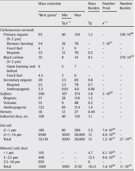
1.3: Major types, sources and mass burdens of particulate matter (adapted from Andreae and Rosenfeld, 2008). 7

1.4: Marine aerosol formation: picture of bubble bursting (1.4a) and schematic (1.4b). 9 1.5: Example of Saharan dust transport as reported by the Moderate Resolution Imaging Spectroradiometer (MODIS) on 16th_{July 2003. 10}

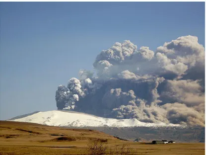
1.6: Volcanic ash being erupted by Eyjafjallajökull (Iceland) in April 2010. 11

1.7: Schematic description of secondary aerosol formation and processing in the marine environment (from Quinn and Bates, 2011). 14

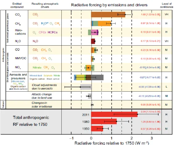
1.8: Global mean radiative forcings as estimated by the fifth Assessment Report of the Intergovernmental Panel for Climate Change (IPCC) in 2013. 17

1.9: Atmospheric aerosol particle modes (adapted from Hinds, 1999). 20

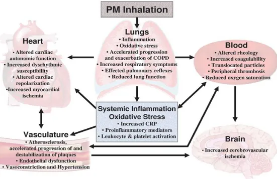
1.10: Potential general pathophysiological pathways linking PM exposure with cardiopulmonary morbidity and mortality (from Pope and Dockery, 2006). 22

1.11: Average PM2.5 (left) and predicted average gain in life expectancy (months) for persons 30 years of

age and older in 25 Aphekom cities for a decrease in the average annual level of PM2.5 to 10 μg m-3

(right). Picture from Aphekom (2011). 22

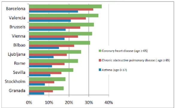
1.12: Percentage of population with chronic diseases due to living near busy streets and roads in 10 Aphekom cities (from Aphekom, 2011). 23

2.1: Variation of the drag coefficient with the particle Reynolds number (adapted from Hinds, 1999). 28 2.2: Schematic of an impactor. Adapted from Vincent (1989). 31

2.3: Particle dispersion due to Brownian motion (from Hinds, 1999). 33

2.4: Difference in visibility due to different aerosol concentrations in Beijing. 34

2.5: Schematic of scattered light including scattering angle, scattering plane and polarised components (i1

and i2). Adapted from Hinds (1999). 34

2.6: Mie intensity parameters versus scattering angle for water droplets (m=1.33) having α=0.8, 2.0 and 10.0 (adapted from Hinds, 1999). 37

2.7: Relative scattering (Mie intensity parameter: i1+i2) versus size parameter for water droplets (m=1.33)

at scattering angles of 30° and 90° (adapted from Hinds, 1999). 37

2.8: Extinction efficiency versus particle size (adapted from Hinds, 1999). 39 2.9: Capture by interception (from Hinds, 1999). 42

2.10: Capture by impaction (from Hinds, 1999). 42 2.11: Capture by diffusion (from Hinds, 1999). 42

(12)

XII

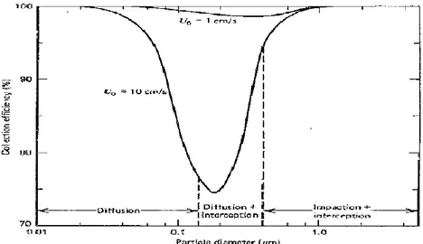
2.12: Filter efficiency versus particle size for different face velocities, t = 1 mm, α = 0.05 and d = 2 μm (from Hinds, 1999). 43

2.13: Predicted alveolar, tracheo-bronchial, head airways and total deposition for light exercise (nose breathing) based on a deposition model (from Hinds, 1999). 45

2.14: American conference of governmental industrial hygenists sampling criteria for inhalable, thoracic and respirable fractions (adapted from Hinds, 1999). 45

2.15: Particle deposition along the respiratory apparatus. 46

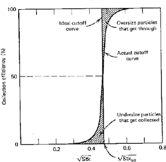
2.16: Example of an impactor cutoff curve: it represents the plot of the impactor's collection efficiency versus the square root of Stk (from Hinds, 1999). 47

2.17: Schematic of a cascade impactor (from Hinds, 1999). 48 2.18: Schematic of a virtual impactor (from Hinds, 1999). 48 2.19: PM sampling station. 49

2.20: Schematic of a Differential Mobility Analyser (from Hinds, 1999). 51 2.21: Scanning Mobility Particle Sizer. 51

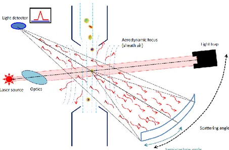
2.22: Schematic of an OPC. Adapted from Colombi et al. (2012). 53

2.23: Theoretical response and experimental calibration curve of the Bausch and Lomb 40-1A particle counter (from Liu, 1976). 55

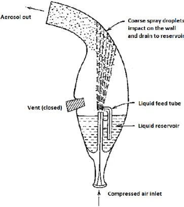
3.1: Diagram of the DeVilbiss mod. 40 nebuliser. Adapted from Hinds (1999). 60 3.2: Projet aerosol generator, Artsana S.p.a. 62

3.3: AGK 2000 aerosol generator, Palas GmbH. 63 3.4: Schematic of AGK 2000, Palas GmbH. 63

3.5: Portable Laser Aerospectrometer Dust Monitor. 65 3.6: Compact OPC N1, Alphasense. 66

3.7: Laser Particle Sensor mod. 3715-00, Kanomax. 67

4.2: Experimental setup for measuring the background concentration in clean air conditions. 73 4.3: Schematic of Test 1. 75

4.3: Particle size distribution as read out from the COPC during Test 2. 75 4.4: Same as Figure 4.3, read out from the GRM. 76

4.5: Experimental setup of Test 4, 5 and 6 76

4.6: Trend of the LPS/GRM ratio in the 0.5-5 μm size range versus the particle number concentration recorded by the GRM during different tests. 77

4.7: Same as Figure 4.6, for COPC/GRM ratio. 78 4.8: Same as Figure 4.7, in the 0.4-0.5 μm size range. 78 4.9: Same as Figure 4.6, for COPC/LPS ratio. 79 4.10: Diagram of the experimental apparatus. 82

(13)

XIII

4.11: Experimental setup. 83

4.12: Particular of a filter's sample. 83

4.13: PSL particle size distribution as read out from the GRM in different channels. 85 4.14: Same as Figure 4.12, for the following test. 86

4.15: Averaged particle size distribution reported by the GRM during the generation of 0.5 μm PSL spheres. 86

4.16: Same as Figure 4.15, reported by the COPC. 87

4.17: Plot of the COPC/GRM ratio in the 0.4-0.5 um size range as a function of the PSL number concentration measured by the GRM in the same range during tests with 0.5 μm PSL. 88 4.18: sample of a stub: a PSL particle of 1 μm in size. 89

4.19: 0.95 μm PSL size distribution as read out from the GRM. 90

4.20: Averaged particle size distribution reported by the COPC during the generation of 0.95 μm PSL spheres. 91

4.21: Same as Figure 4.20, reported by the GRM. 91

4.22: Plot of the normalised particle number concentations reported by the COPC and the GRM as read out from each channel against the corresponding particle size during the test with 0.5 μm PSL spheres conducted with the Projet nebuliser. 92

4.23: Same as Figure 4.22, during tests with 0.95 μm PSL spheres. 92 4.24: LPS, COPC and GRM during the sampling. 93

4.25: 0.5 μm PSL particle size distribution achieved with the AGK 2000 generator as reported by the GRM. 94

4.26: Same as Figure 4.25, reported by the COPC. 94

4.27: Same as 4.17, with results from the AGK 2000 generator too. 95

4.28: 1.03 μm PSL particle size distribution achieved with the AGK 2000 generator as reported by the COPC. 95

4.29: Same as Figure 4.28, reported by the GRM. 96

4.30: Same as Figure 4.22, during tests conducted with the AGK 2000 generator. 97 4.31: Same as Figure 4.23, during tests conducted with the AGK 2000 generator. 97

4.32: Time-series of the particle number concentrations in the 0.4-5 um size range during Test A. 99 4.33: Scatterplot of the GRM output against the COPC output for the 0.5-5 um size range during Test A. 99

4.34: Same as Figure 4.32, during Test B. 100 4.35: Same as Figure 4.33, during Test B. 101

4.36: Time-series of the particle number concentrations in the 1-5 um size range during Test A. 102 4.37: Same as Figure 4.36, during Test B. 102

(14)

XIV

4.38: Scatterplot of COPC/GRM as a function of the GRM particle number concentration during Test A for the 0.4-5 μm size range. 103

4.39: Same as Figure 4.38, during Test B. 103

5.1: Electronic components of the Laser Particle Sensor mod. 3715-00. 107 5.2: Measuring the voltage between TP3 and TP GND (V3). 108

5.3: Laser Particle Sensor mod. 3715-00 connected to mini-BUCK calibrator mod. M-5. 109 5.4: Particular of the LPS's internal circuit: pins. 110

5.5: Experimental setup for the calibration of the LPS’s counting efficiency. 112

5.6 Plot of the counting efficiency against VPIN2 for the 0.5-5 μm size range while generating 0.5μm PSL

(15)

XV

List of tables

1.1: EU Standards for Particulate Matter for PM10 and PM2.5 (from Air Quality Standards). 18 3.1: Specifics of the Portable Laser Aerospectrometer Dust Monitor. 65

3.2: Channel division of the Portable Laser Aerospectrometer Dust. 65 3.3: Specifics of the CompactOPC N1, Alphasense. 66

3.4: Channel division of the Compact OPC N1, Alphasense. 66

3.5: Specifics of the Laser Particle Sensor, mod. 3714-00 and 3715-00. 67

4.1: Particle number concentration measured by each OPC in clean air conditions. 73 4.2: Configuration setup of each indoor sampling. 74

4.3: Particle number concentrations as read out from each instrument in the 0.4-0.5 μm and 0.5-5 μm size ranges in each sampling. 77

4.4: Response times of each OPC in different size ranges. 81

4.5: Particle counts in each observed field of the three filter's samples. 84

4.6: Particle number concentrations measured by each OPC and obtained by counting the particles deposited onto the filter. 87

4.7: COPC/GRM, LPS/GRM and COPC/LPS ratios for the 0.4-0.5 μm and 0.5-5 μm size ranges during the nebulisation of PSL spheres of 0.5 μm in diameter. 87

4.8: Comparing the PSL number concentration evaluated from filter data with the ones read out from each OPC. 90

4.9: Particle number concentrations reported by each instrument in several size ranges during the test with 1.03 μm PSL spheres conducted with the AGK 2000 generator. 96

5.1: LPS's sample flow rate after the calibration: details on the single measurements. 109 5.2: Voltage output and note of each pin. 111

(16)

(17)

1

Introduction

The term aerosol, or particulate matter (PM), defines a colloidal mixture where liquid and solid particles are suspended in the air. Atmospheric aerosol particles, in particular, have different physical and chemical properties, which depend on sources and atmospheric transformation. Classifications of atmospheric aerosols are based on the particle size, the origin (i.e., where the aerosol was generated) and the source (i.e., whether it is a primary or a secondary aerosol). From the physical viewpoint the size, typically ranging from 0.001 up to 100 μm, is the most important parameter for the characterisation of an aerosol particle.

Atmospheric aerosols may be of natural or anthropogenic origin and may either be directly emitted by the source (primary aerosol) or result from chemical transformations in the atmosphere (secondary aerosol).

Marine aerosol, mineral dust, volcanic ash and primary biological particles are classified as natural aerosols. The main compositions of such aerosols are: inorganic salts (marine aerosol), crustal elements (mineral dust and volcanic ash), natural microorganisms such as fungi or spores (primary biological organic particles), nitrates and sulphates (volcanic ash).

Anthropogenic aerosols are the result of several human activities, such as agriculture, industrial processes, transports, waste disposal and heating systems. Such aerosols mostly contain carbon, sulphates, nitrates and mineral elements.

Secondary aerosols may be either organic or inorganic and are particles resulting from transformation processes of substances of both natural and anthropogenic origin.

Aerosols are also found in indoor environment: cigarette smoke, wood-burning stoves, kerosene heaters, carpets, pressed wood furniture and household cleaning products are typical sources of indoor aerosols. Particles from such sources are mostly composed by carbon, nitrogen and metals.

Aerosols play an important role in most of the atmospheric microphysical, chemical and photochemical processes, thus affecting the Earth’s climate. Due to their sizes, aerosol interact with the incoming solar radiation, thus yielding the so-called aerosol’s direct effect; as aerosols mostly scatter rather than absorb the solar radiation, the global net effect is a cooling at the Earth’s surface. Aerosols can also act as condensation and ice

(18)

2

nuclei for cloud formation, thus changing their radiative properties and lifetime. This is called the aerosol’s indirect effect.

Aerosols can be inhaled by the human airways apparatus and have therefore an important effect on human health, with decreases in life expectancy observed in places with huge aerosol concentrations, such as big cities. Smaller particles are associated with the strongest impairing effects as they can penetrate inside the airways system more deeply than coarse particles. Therefore, it is of primary importance to monitor aerosol concentration and size distribution on a real-time basis to assess their effects on both climate and human health.

Optical Particle Counters (OPCs) can classify particles from 0.3 μm up to 20 μm; they rely upon light scattering to measure particle size distributions and particle number concentrations (i.e., particles amount per unit volume) on a real-time basis. As they are small and handy, they are widely used for sampling aerosols.

New generation OPCs are even smaller and cheaper with respect to the traditional devices deployed so far in air quality studies and are therefore best suited for personal exposure assessment to particulate and for indoor aerosol characterisation. They might also be used in participatory monitoring networks or in distributed sensor networks (smart cities). However, OPCs require frequent calibrations, which are usually performed by producing aerosol particles of controlled size by means of a nebuliser and testing the response of the OPC against a reference device (which may be a calibrated instrument) or against an absolute particle concentration value. The latter is obtained by directly counting particles deposited onto filters sampling in parallel to the OPC at a Scanning Electron Microscope (SEM).

The aims of this thesis are:

1) to characterise a novel OPC (CompactOPC N1, produced by Alphasense; hereafter COPC) in terms of counting efficiency and size classification against a standard commercial OPC (Portable Laser Aerosolspectrometer Dust Monitor Model 1.108, produced by GRIMM AEROSOL Technik GmbH & Co.; hereafter GRM);

(19)

3

2) to set up a test bench for calibrating an OPC used in clean room and sanitary environments (Laser Particle Sensor mod. 3715-00, produced by Kanomax; hereafter LPS).

The LPS is distributed in Italy by Pollution Clean Air Systems S.p.A and at the present day its calibration is not carried out in Italy. Pollution Clean Air Systems S.p.A (Budrio, BO) is keen on carrying out this activity for its customers. Therefore, the company is interested in the results of this work as a potential improvement of its customer service and as an example of cooperation between research centres and small or medium enterprises.

The work is divided in five chapters. Chapter 1 provides a summary of aerosol sources and the effects of aerosols on climate and human health. Chapter 2 includes a review of aerosol physics and instrumentation for measuring and characterising aerosol particles, with a special focus on OPCs. Chapter 3 deals with the instrumentation used to perform the experimental part of the work: aerosol generators, OPCs used in the research and SEM analysis protocol are described. The methodology to determine mean values and experimental errors from OPC and SEM output is also provided. In Chapter 4 results are shown for tests with indoor aerosol and calibrated aerosol particles. An improvement of deploying the COPC in terms of aerosol sampling efficiency is also included. Finally, Chapter 5 provides details and experimental results for the calibration bench of the LPS.

(20)

(21)

5

Chapter 1: Aerosol sources and properties

1.1 Introduction

The term aerosol defines a colloidal mixture where liquid and solid particles are suspended in a gas. Atmospheric aerosol particles, in particular, have different physical and chemical properties (size, shape, chemical composition, refractive index, etc…), which depend on sources and atmospheric transformation.

From the physical viewpoint the size is the most important parameter for the characterisation of a particle. Particle sizes can range from 0.001 up to 100 μm, which accounts for five magnitude orders between the smallest and the biggest particles. The common reference for particle size is the particle diameter (Hinds, 1999).

The concentration of aerosols in the atmosphere can be defined as particle mass

concentration (the total mass of the particles per air unit volume, expressed in μg m-3_{), or}

particle number concentration (the number of particles per unit volume).

Common classifications of the aerosol particles are in terms of particle size, origin (i.e., where the aerosol was generated) and source (i.e., whether it is a primary or a secondary aerosol). Nevertheless further classifications may exist if required in special problems. Figure 1.1 reports the size of some of the main aerosol types and provides insight into their relative weight in contributing to the total particulate mass fraction. Figure 1.2 reports the yearly average aerosol optical thickness at λ = 0.55 μm over Europe as measured by the Moderate-Resolution Image Spectroradiometer (MODIS). As the picture suggests, the greatest aerosol emissions are mostly correspondent to industrialised areas (e.g., the Po Valley) and deserts. The main types, sources and mass burdens of particulate matter are finally summarised in Figure 1.3.

(22)

6

Figure 1.1: Particulate matter size distribution (from Hinds, 1999).

Figure 1.2: Yearly average aerosol optical thickness over Europe (at 0.55 μm) measured by MODIS in 2003. White: missing data. Picture from Koelemeijer et al. (2006).

(23)

7

Figure 1.3: Major types, sources and mass burdens of particulate matter (adapted from Andreae and Rosenfeld, 2008).

1.2 Atmospheric aerosol

Aerosols have either natural or anthropogenic sources and may either be emitted as primary particles (i.e., they are directly injected into the atmosphere) or result from secondary processes (i.e., by transformation of precursor gases).

1.2.1 Natural aerosol

The natural aerosol is commonly regrouped in four classes: marine aerosol, mineral dust, volcanic ash and primary biological aerosol particles (PBAP).

(24)

8

1.2.1.1 Marine aerosol

The marine aerosol is the aerosol confined in the marine boundary layer, mostly generated from sea spray. However, the marine environment also comprises other particles, such as sulphates from biogenic and anthropogenic sources (Andreae and Rosenfeld, 2008). Sea salt or sea spray aerosols are generated by bubble bursting from breaking waves and capillary action at the ocean surface due to the stress exerted by the surface wind, which largely affects the production rate. The size of such particles ranges from the submicrometer interval up to some μm, the smallest particles being associated with film droplets (0.3 μm in diameter on average) and the biggest particles being associated with jet droplets (size greater than 2 μm). Figure 1.4b is a schematic of bubble bursting and shows the difference between film and jet droplets, while Figure 1.4a is a representation of the process.

The generated aerosol particles can scatter light and act as cloud condensation nuclei. Therefore, they may affect cloud physics and the radiation budget in the atmosphere. Furthermore, they interact with anthropogenic pollution and affect gas chemistry and biogeochemical cycles in marine and terrestrial ecosystems.

The primary component of sea spray is given by a mixture of inorganic salts, of which NaCl is the most prominent in mass concentration. An organic component is also present, coming from the sea surface and gas phase oxidation of volatile organic compounds (VOCs), that lead to formation of secondary organic aerosol.

Many organic compounds are found in the sea water, mostly originated by degradation of marine organisms and plants and therefore consists of amino- and fatty acids, carbohydrates, saccharides and cell fragments.

Marine aerosols can also serve as sink for reactive gases and small particles, as well as suppress new particle formation (Fuzzi, 2015).

(25)

9

1.2.1.2 Mineral dust

Mineral dust comprises all kinds of particles that are suspended in the atmosphere mostly originated by the action of the wind (erosion of rocks or updraft and transport of powders over long distances). According to Ginoux et al. (2012), this aerosol is mostly (75%) emitted by natural sources and the remaining part is due to anthropogenic emissions (primarily agricultural).

This kind of aerosol affects climate through direct and indirect effects, modifies marine biogeochemistry and affects human health. Specifically, the intrusion of Saharan dust accounts for some of the annual PM10 daily exceedances in Southern Spain and in general in the Mediterranean area (Rodriguez et al., 2001; Monks et al., 2008). Figure 1.5 shows an example of Saharan dust transport from Northern Africa to Southern Europe.

Typical components of mineral dust are crustal elements such as Fe, P, Na, Ba, Br, Mg, Al, K, Ca, Ti, Cu and V (Chen et al., 2008).

Aerosols in soil dust absorb visible radiation, thus yielding an atmospheric warming, while scattering by mineral dust leads to surface cooling Aerosols in soil dust absorb visible radiation, thus yielding an atmospheric warming, while scattering by mineral dust leads to surface cooling. These two processes affect climate and wind circulation on a regional scale through a reduction of downward mixing of momentum within the planetary boundary layer, the surface wind and, thus, dust emission (IPCC, 2013). As an example, atmospheric warming over the Sahara regions causes an intense heat pump effect that increases precipitation over the northern Sahel.

Figure 1.4a: The wind's action causes bubble bursting at the sea surface and leads to the production of sea spray.

Figure 1.4b: Schematic of marine aerosol formation. Small particles (some tenths of μm on average) are associated with film drops (left), while big particles (some μm) are associated with jet drops (right).

(26)

10

As mineral dust contains micronutrients like Fe and P, it intervenes in the ocean-carbon cycles, thus affecting the exchange of CO2 and creating dust-climate feedback mechanisms.

Figure 1.5: Example of Saharan dust transport as observed by the Moderate Resolution Imaging Spectroradiometer (MODIS) on 16th July 2003. This a clear demonstration of the combined action of the wind and the atmospheric circulation that may lead to severe outbreaks of Saharan dust towards Europe.

1.2.1.3 Volcanic ash

Volcanic ash is a particular type of mineral dust. It consists of pulverised materials (rocks, dust and volcanic glass) dispersed by explosive volcanic eruptions. Volcanic ash is formed when dissolved gases in magma expand and escape violently into the atmosphere, where they solidify and become aerosol.

Just like mineral dust, typical components of volcanic ash are crustal elements (mostly Ca, Na, Al and Fe), as well as nitrates and sulphates that are mainly suspended in the volcanic gases (Schleicher et al., 2010).

Volcanic dust from explosive eruptions is known to affect climate over periods ranging from a few months up to some year. During an explosive eruption, volcanic ash plumes can acquire velocities up to 100 m s-1, reach the tropopause and enter the stratosphere. An intense volcanic activity yields an increase in the atmospheric optical depth in the stratosphere, which results in a net cooling at the Earth’s surface. Apart from large particles, which are removed by gravitational settling, most of the aerosol particles can remain in suspension above the tropopause for several months.

(27)

11

The atmospheric circulation can transport volcanic ash over long distances. For instance, some weeks after the Eyjafjallajökull (Iceland) eruption in 2010 (see Figure 1.6), PM measurements carried out in Bologna with a DMPS (see Chapter 2.4.3) and an OPC (see Chapter 2.5.2) revealed an increase in concentration of the accumulation and the coarse fraction during the transit of the ash cloud (Belosi et al., 2011).

The extent in time and space of a climate anomaly due to an eruption mostly depends on the amount of materials injected into the atmosphere, as well as where the eruption takes place. It is known that 1816 is considered “the year without summer” due to the eruption of Mount Tambora in 1815 (Stothers, 1984). Particularly in the northern hemisphere, the summer season was characterised by unusually low temperatures, often associated with severe weather events, in some cases snowfalls, like in New England (Canada).

Figure 1.6: Volcanic ash being erupted by Eyjafjallajökull (Iceland) in April 2010.

1.2.1.4 Primary Biological Aerosol Particles (PBAP)

PBAP includes components with a large range of size, such as microorganisms (bacteria, fungi, algae), fungal spores, pollen, viruses, biological fragments that are directly emitted to the atmosphere from their sources, as well as debris. Typical size ranges are: 0.05-0.15 µm for viruses, 0.1-4 µm for bacteria, 0.5-15 µm for fungal spores and 10-30 µm for pollen.

Bacteria and other bioaerosols may attach to other particles, be transported with them, and change the size distributions of such particles (Pastuszka et al., 2000).

(28)

12

PBAP intervene in ice nucleation and cloud drop formation and can affect climate and the hydrological cycle on regional and, perhaps, global scale. Moreover, they may cause harmful health effects (allergies, asthma, infectious diseases, etc.)

1.2.2 Anthropogenic aerosol

Anthropogenic aerosol can derive from: industrial processes, agricultural activity, transports (roads, ships, rail, air), and waste disposal. A significant part also derives from non-exhaust emissions, such as abrasion of tyre wear, brake wear, road wear and road dust suspension induced by road transport.

Exhaust particles mostly contain carbon compounds, sulphates and nitrates and are usually fairly smaller (they mostly account for the PM2.5 mass fraction; see Chapter 1.4.2) compared to the non-exhaust ones. Instead, the latter mostly contain metals, metal oxides and mineral elements and present less carbonaceous material.

Wood combustion is a special case of exhaust emissions as it is mostly used for residential heating. Hence it gives an important contribution to the organic aerosol fraction and it is mostly responsible for high PM values in wintertime (e.g., Szidat et al., 2006). Most of these particles consists of highly soluble material and can therefore act as condensation nuclei.

Depending on the composition, the anthropogenic aerosol can either mostly absorb (as in the case of carbon compounds that account for the black carbon fraction) or scatter (nitrates and sulphates) solar radiation. Observations suggest that the net contribution to the radiation forcing is on average negative, although great uncertainties exist (Wang et al., 2013).

Datasets or inventories on each single source are not entirely available and are often incomplete as the amount of aerosol produced by such processes is not easy to evaluate and only partial estimates are available.

1.2.3 Background and secondary aerosol

The term secondary aerosol refers to the particles that are not directly injected into the atmosphere. Secondary aerosol can be inorganic and organic. Secondary inorganic aerosol is formed prevalently from oxidation reaction of NOx and SO2.

(29)

13

SO2 sources can be anthropogenic and natural. Oxidation of SO2 with formation of sulphuric acid can occur in the gas phase and in the liquid phase, e.g. cloud or fog. Once formed in the atmosphere sulphuric and nitric acids show very different behaviour, both physically and chemically. Nitric acid is more volatile and hence exists in significant concentrations in the gas phase, while sulphuric acid has a very low vapour pressure. Once formed, vapour molecules rapidly transfer to the particulate phase by nucleation or condensation on existing aerosol surface. These processes are schematically represented in Figure 1.7.

Both sulphuric acid and nitric acid react with atmospheric ammonia. However gaseous ammonia first reacts with sulphuric acid to form ammonium bisulphate and ammonium sulphate, then the remaining free ammonia is depleted by reaction with nitric acid to form ammonium nitrate.

In addition to anthropogenic sources, in marine environment there is also a contribution to sulphates from the oxidation of dimethylsulphide (DMS) produced in seawater from the activity of various phyto- and zoo-planktonic species. Once released into the atmosphere DMS will follow an oxidation scheme controlled principally by hydroxyl radical (OH.) during the day and nitrate radical (NO3) at night, thus producing sulphates and methanesulphonic acid (MSA). As a matter of a fact, MSA can be considered an indicator for DMS particulate oxidation products.

Secondary organic aerosol is formed in the atmosphere through reactions that transform volatile organic compounds (VOC) into low-vapour-pressure compounds, followed by condensation on existing particles, or by homogeneous nucleation (transition phase in the absence of a condensation nucleus).

The photochemical action of bright sunlight on nitrogen oxides (NO and NO2) and VOCs leads to the formation of most of the ultrafine fraction. Both components are mostly of anthropogenic origin and the result of this process is called the photochemical smog and involves the interaction of sunlight with particles of different origins such as: exhaust emissions from vehicles and industries, forest fires, volcanic action, lightning, bacterial action in soil.

(30)

14

Figure 1.7: Schematic description of secondary aerosol formation and processing in the marine environment. Picture from Quinn and Bates (2011).

1.3 Indoor aerosol

The term indoor aerosol includes all kinds of suspended particulate matter that are found in indoor environments. In practice, the greatest difference between indoor and outdoor aerosol is given by the sources, while the chemical composition is often similar.

In developed countries, people spend most of their time indoors and several studies (Tan et al., 2012; Wang et al., 2007) have shown that indoor pollutant levels can be on average two to five times higher than their corresponding outdoor ones. As a matter of a fact, indoor air pollution is responsible for 2.7% of the total burden of disease and worldwide one million people per year die from pulmonary diseases due to the exposure to indoor smoke (Fang et al., 1999; Hetland et al., 2000).

Cigarette smoke, wood-burning stoves and kerosene heaters, carpets, pressed wood furniture and household cleaning products are typical sources of particulate matter in indoor environments (Daisey and Gundel, 1991; Tan et al., 2012). Emissions by these sources usually include organic carbon, elemental (black) carbon, nitrogen and metals (Fe, Na, Zn).

Bioaerosols such as fungi and bacteria are mostly found in mouldy and crowded environments: in conditions of high humidity rates and poor ventilation, microbiological

(31)

15

organisms can easily grow and develop (Pastuszka et al., 2000). Such particles are a major cause of respiratory diseases in indoor environments.

Ventilation and air-conditioning systems can favour microbial growth, while several types of microorganisms are used to produce pharmaceutical products, enzymes and food substitutes in commercial laboratories.

Indoor aerosol also includes biological emissions by plants, toner particles and suspensions from nebulising devices for medical or experimental (e.g., polystyrene latex) use. However, the most important sources of indoor particulate matter are probably cooking and heating. In particular, the exposure to indoor PM is higher in the dwellings of people with medium or low resources in developing countries, where solid fuels (biomass and coal) are widely deployed for cooking and heating purposes (Abdullahi et al., 2013).

Visible fumes are mostly submicrometer-sized particles mostly consisting of oil, combustion products, steam and condensed organic pollutants (Abdullahi et al., 2013); other products are volatile organic and nitrogen-related aerosols (Daisey and Gundel, 1991). The particulate matter relative to cooking processes is mostly in the ultrafine (less than 100 nm in diameter) and fine (aerodynamic diameter smaller than 2.5 μm) particle range. Particles from indoor combustion are a major cause of pulmonary diseases and most of them also possess mutagenic properties (Daisey and Gundel, 1991).

1.4 Aerosol effects

1.4.1 Climate effects

As already mentioned, aerosols are an integral part of the atmosphere and play an important role in most of the atmospheric microphysical, chemical and photochemical processes. Several feedback mechanisms are therefore established, most of which are complex and currently not fully understood.

Due to their sizes, aerosols interact with both longwave (LW) and shortwave (SW) radiation. In particular, they can always scatter and, in some cases, also absorb the incoming radiation. Physical properties of particles, like the extinction coefficient and the scattering phase function, depend on the wavelength of the incoming radiation and on the

(32)

16

atmospheric relative humidity, while the atmospheric loading and the geographic distribution of aerosols are determined by the atmospheric dynamics. As the result in terms of incoming radiation is directly determined by the interaction between aerosols and solar radiation, this is called the aerosol’s direct effect.

Scattering aerosols always exert a negative radiative forcing (i.e., they cause a decrease in the incoming solar radiation at the ground, thus inducing a decrease in the temperature), while absorbing aerosols may exert both a positive or a negative radiative forcing, depending on whether they are located on a bright surface (like a snow-covered surface or a bright cloud, thus yielding a positive forcing) or a dark surface (such as oceans or forests, thus yielding a negative forcing).

If an aerosol is located at the top of the atmosphere (TOA), whether it can or cannot absorb, the net effect is always a reduction of SW irradiance at the surface. If it can absorb, the effects of the positive radiative forcing induced by the aerosol will be only observed in the layer where the aerosol lies. As an example, an increase in stratospheric SO2 due to intense volcanic activity yields a net stratospheric warming, while the underlying layers will experience a net cooling.

The so-called aerosol’s indirect effect refers to the mechanisms by which aerosols modify the microphysical and hence the radiative properties and the lifetime of clouds. Size, chemical composition, mixing ratio and surrounding environment determine if an aerosol can act as a condensation nucleus for clouds, as well as an ice nucleus.

By affecting the cloud droplet number concentration, the aerosol modifies the cloud albedo. By keeping the cloud liquid water content unaltered, a high aerosol concentration, as it might be found in polluted regions, can determine a high concentration of small cloud droplets, thus increasing the cloud reflectivity, i.e. the albedo.

By affecting the cloud liquid water content and the cloud height, the aerosol modifies the cloud lifetime. High concentration of small droplets leads to decreased drizzle production and reduced precipitation efficiency.

According to the 5th Assessment Report of the Intergovernmental Panel for Climate Change (IPCC), issued in 2013, on a global scale aerosols are estimated to account for the greatest cooling contributions (-0.27 W m-2 as a mean net contribution) and the level of confidence relating to the aerosol direct effect is classified as high. On the other hand, the aerosol indirect effect provides a greater cooling contribution (-0.55 W m-2_{), but its}

(33)

17

level of confidence is classified as low. Figure 1.8 reports the net contribution and the level of confidence associated with each forcing.

From a modelling perspective, the largest uncertainties in a model-predicted climate change are due to the aerosol emissions in future scenarios. Just like in the case of greenhouse gases, estimates of future aerosol concentrations can be made based on economical and political considerations. However, due to the limited knowledge of most of the aerosol-related feedback mechanisms, any prediction of future climate change should be taken with caution.

Figure 1.8: Global mean radiative forcings as estimated by the 5th_{Assessment Report of the Intergovernmental Panel}

for Climate Change (IPCC) in 2013. Diagrams bending on the right imply a positive forcing (warming), while diagrams bending on the left imply negative forcing (cooling). A level of confidence is associated with each forcing (from IPCC 5th_{Assessment Report, 2013).}

1.4.2 Health effects

Since the Industrial Revolution it was realised that an increase in particulate emission was often associated with a decrease in the quality of life in terms of diseases. Before then, only miners or scavengers could be aware of the negative effects of inhaling large

(34)

18

amounts of dust or smoke. To the present day evidences suggest links between aerosols and cardiovascular, pulmonary and airway diseases (Pope and Dockery, 2006).

Due to the effects aerosols exert on the human health, the European Union and the U.S.A. have issued directives for aerosol standards: the EU Standards for Particulate Matter (PM10 and PM2.5), reported in Table 1.1, and the National Ambient Air Quality Standards (Putaud, 2003; NAAQS; Air Quality Standards). These directives impose limits to the daily and yearly PM mass concentrations and therefore to the emissions of particulate matter by traffic and industries.

Concentration [μg/m3]

Averaging time Entrance into force of the limit value

Permetted exceedances per year PM10 ₅₀ _{24 hrs} _01/01/2005 ₃₅ 40 1 year 01/01/2005 n/a PM2.5 25 1 year 01/01/2015 n/a

Table 1.1: EU Standards for Particulate Matter for PM10 and PM2.5 (from Air Quality Standards).

The term PM10 (PM2.5) refers to the mass concentration of particles with an aerodynamic size smaller than 10 µm (2.5 μm), whatever the particle origin, source and chemical composition. The classification of particles by their aerodynamic diameter is mostly for conventional and air monitoring purposes as the aerodynamic size determines the transport and removal of particles from air, the particle chemical composition and, most importantly, the particle deposition inside the respiratory system (CAFE, 2005).

In urban environments, particles are usually divided into two groups: coarse particles and fine particles. The border between these groups lies between 1 and 2.5 μm in aerodynamic diameter. For measurement purposes, the term PM2.5 indicates the fine fraction, while the term PM10 refers to the coarse fraction.

Figure 1.9 reports the three modes by which atmospheric aerosol is usually classified. By looking at the particle volume, which is directly linked to the particle mass, the coarse mode and the accumulation mode are clearly visible. Particles of the coarse mode are generated by breakup of larger solid particles, mostly due to windblown dust from agricultural processes, mining operations and uncovered soil. Other sources of coarse particles are traffic emissions, sea spray, pollens and fungal spores.

(35)

19

suspended particulate, but when considering the particle number concentration they account for a very small fraction. On the contrary, while fine particles account for a very small fraction of the total PM mass (1-8%), they appear to be the most important contributor for the PM number concentration. Ultrafine particles (less than 0.1 μm in diameter), also known as Aitken mode particles, are mostly generated by gas-to-particle conversion and nucleation. An example of these processes is provided by Diesel engines, which are a major source of ultrafine particles in urban environments (Giechaskiel et al, 2014; Reşitoğlu and Altinişik, 2015).

Once formed, ultrafine particles grow by condensation (gas condensation onto the surface of existing molecules) or coagulation (two or more particles combining to form a bigger one) and generate the so-called accumulation mode (around 0.1 μm in diameter).

Fine particles (PM2.5) appear to be strongly associated with mortality and hospitalisations due to cardio-vascular diseases; in particular, ultrafine particles (less than 0.1 μm in diameter) are associated with negative health effects.

Ultrafine particles are however thought to be the most harmful because of their porous surface and their large surface area due to their large number concentration, which allows them to adsorb toxic substances (Valavanidis et al., 2008). In particular, as they deposit by diffusion in all parts of the respiratory tract, through the blood and lymph circulation they can easily reach potentially sensitive target sites such as bone marrow, lymph nodes, spleen, and heart (Obersdörster et al., 2005).

(36)

20

Figure 1.9: Atmospheric aerosol particle modes (adapted from Hinds, 1999).

A schematic of how PM is inhaled and interact with the human body is reported in Figure 1.10. In particular, it is thought that inhaled particles may affect the behaviour and characteristics of blood, lungs, heart, vasculature and brain.

As for the exposure period, short-term exposures to ambient PM in highly polluted areas may lead to general airways disturbances, the greatest effects being more remarkable in elderly subjects and people with pre-existing heart and lung diseases, who are usually more susceptible to the PM effects on mortality and morbidity (Fowler et al., 2012). On the other hand, long-term exposures to high PM levels may lead to a reduction in life expectancy by a few months up to a few years due to cardio-pulmonary diseases, lung

(37)

21

cancer and generic reduced lung function. The Aphekom project has issued a summary report for the impact of the air pollution on health in Europe for the period 2008-2011. Figure 1.11 shows the average PM2.5 level and describes the forecast increase in life expectancy in 25 cities of the survey in case of decrease of PM2.5 concentration down to 10 μg m-3_{, while Figure 1.12 shows the percentage of the population in 10 different cities} affected by chronic diseases due to living near busy streets and roads (Aphekom, 2011). As reported by Pope and Dockery (2006), major effects due to PM exposure are found in socially disadvantaged and poorly educated populations, with no differences between men and women and between smokers and non-smokers. In any case, a strict dependency of the death rates on the exposure’s time-scale and the PM level is observed.

Some of the features contributing to toxicity are the metal content, the presence of polycyclic aromatic hydrocarbons and an extremely small size. Sources associated with health effects include combustion engines, coal burning and wood burning. Particles from these sources mostly belong the fine and ultrafine fraction and appear to have a strong inflammatory potential.

Finally, carbonaceous and metal particles often present mutagenic activity (Pastuszka et al., 2000; Valavanidis and Vlachogianni, 2008).

Biogenic particles such as fungi, fungal spores or bacteria are often associated with respiratory disturbances like asthma (Pastuszka et al., 2000), which can be exacerbated by a prolonged exposure.

(38)

22

Figure 1.10: Potential general pathophysiological pathways linking PM exposure with cardiopulmonary morbidity and mortality (from Pope and Dockery, 2006).

Figure 1.11: Average PM2.5 (left) and predicted average gain in life expectancy (months) for persons 30 years of age

and older in 25 Aphekom cities for a decrease in the average annual level of PM2.5 to 10 μg m-3 (right). Picture from

(39)

23

Figure 1.12: Percentage of population with chronic diseases due to living near busy streets and roads in 10 Aphekom cities (from Aphekom, 2011).

(40)

(41)

25

Chapter 2: Aerosol physics and applications

2.1 Aerosol mechanics and behaviour

In this chapter the main features of aerosol mechanics and behaviour are reviewed. Starting from kinetic gas theory, Stokes’s resistance law will be enounced and concepts like settling velocity, Stokes number and Brownian diffusion will be introduced and described. Formulas are taken from Hinds (1999).

2.1.1 Ideal gas law and Reynolds number

The gas in which particles are suspended resists particle motion depending on the particle size. For a perfect gas, the kinetic theory of gases and therefore the ideal gas law are valid. The gas at issue is the air, which is approximately an ideal gas and to which the ideal gas law can apply.

The kinetic theory of gases assumes that:

1) gases contain a large number of molecules;

2) molecules are small compared with the distance between them;

3) molecules are rigid spheres travelling in straight lines between elastic collisions.

The ideal gas law follows from these assumptions. It states that at constant temperature T and number of molecules n, the product between pressure and the volume occupied by the gas is constant:

𝑝 𝑣 = 𝑐𝑜𝑛𝑠𝑡𝑎𝑛𝑡

Equation 2.1

or

𝑝 𝑣 = 𝑛 𝑅 𝑇

(42)

26

where n is the molecular concentration and R = 8.314 J mol-1_K-1_{. For the atmosphere, in} the case of dry air, the ideal gas law can be re-written as follows:

𝑝 = 𝜌𝑎𝑅𝑣 𝑇

Equation2.3

where ρa is the air density and Rv = 287 J kg-1 K-1.

Due to the interaction of particles with the gas in which they are suspended, a mean free path λ is defined as the average distance travelled by a molecule between successive collisions.

𝜆 = 𝑐̅ 𝑛_𝑧

Equation 2.4

where 𝑐̅ is the mean molecular velocity and nz is the number of interactions per unit time. The property that indicates how much the gas resists particle motion is called viscosity η. For an ideal gas viscosity is related to the mean free path according to:

𝜂 = 1

3 𝑛 𝑚 𝑐̅ 𝜆

Equation 2.5

where m is the mass of one gas molecule. In terms of molecular energy, viscosity is related to the absolute temperature T by:

𝜂 = 2 (𝑚 𝑘 𝑇) 1 2 3 𝜋3/2_𝑑 𝑚 2 Equation 2.6

where k = 1.38 10-23 _{J K}-1_{is the Boltzmann constant and d}

m is the collision diameter of the molecule, i.e., the distance between the centres of two molecules at the instant of collision; for air dm is approximately 3.7 10-10 m.

(43)

27

Viscosity only depends on gas molecular constants; however Equation 2.6 is only exact for perfect sphere. For most of the temperature ranges of interest, the correct dependency between η and T is T0.74_.

When dealing with fluids, the quantity that provides insight on the flow regime (laminar or turbolent) is the Reynolds number, which is given by:

𝑅𝑒_𝑔 = 𝜌 𝑉 𝑑 𝜂

Equation 2.7

where V is the relative speed between the fluid and a particle, ρ is the density of the fluid and d is a characteristic linear dimension, such as the diameter of a pipe the flow must pass through.

Reg is the ratio of the fluid inertia to the fluid viscosity. Low Reg (less than or approximately 1) indicates laminar flow, while high Reg indicates turbolent flow.

2.1.2 Stokes’s resistance law, Stokes number and settling velocity

When a particle travels in a gas, it will face a resistance force. The force the gas will exert on the particle is given by Newton's resistance law, whose general form is:

𝐹_𝐷 = 𝐶_𝐷𝜋

8𝜌𝑔𝑑2𝑉2

Equation 2.8

where CD is the drag coefficient and ρg is the density of the gas resisting particle motion. The Reynolds number of a particle Rep is given by:

𝑅𝑒_𝑝 = 𝜌 (𝑉𝑝− 𝑉𝑔)𝑑𝑝 𝜂

Equation 2.9

where Vp – Vg is the velocity difference between the particle and the gas and dp is the particle size. For Rep > 1000 Stokes's law is valid.

(44)

28

𝐹_𝐷 = 3 𝜋 𝜂 (𝑉_𝑝− 𝑉_𝑔) 𝑑

Equation 2.10

For Rep < 1, by equating Stokes's law to Newton's law, it may be seen that a relationship exists between CD and Rep.

𝐶𝐷 = 24 𝜂 𝜌𝑔(𝑉𝑝− 𝑉𝑔) 𝑑 = 24 𝑅𝑒𝑝 Equation 2.11

Fig 2.1 shows the particle Reynolds number as a function of the drag coefficient. It is observed that at small Rep (less than 1), CD and Re are inversely proportional, while at high Rep (greater than 1000), CD assumes a nearly constant value of 0.44. Stokes's law is valid for perfect spheres and for incompressible fluids

Figure 2.1: Variation of CD with Rep. For Rep < 1 CD is inversely proportional to Rep (Stokes's region), while for Rep = 103

-105_C_D_{is nearly constant and equal to 0.44. In the middle lies the transition region (adapted from Hinds, 1999).}

When a particle travels inside a gas that resists its motion, if the particle is subjected to an acceleration, at a certain point the resistance offered by the gas will equal the acceleration of the particle. At this point, the velocity of the particle will be constant If the acceleration is provided by the gravitational force, Stokes’s law predicts:

𝐹𝐷 = 𝐹𝐺 = 𝑚 𝑔

(45)

29

3 𝜋 𝜂 (𝑉_𝑝− 𝑉_𝑔) 𝑑 = (𝜌𝑝− 𝜌𝑔)𝜋 𝑑 3_𝑔 6

Equation 2.13

By neglecting ρg as it is usually much smaller than the particle density ρp , one finds the

settling velocity VTS.

𝑉_𝑇𝑆 = 𝜌𝑝𝑑 2_𝑔 18 𝜂

Equation 2.14

VTS rapidly increases with particle size and decreases with increasing viscosity.

Two important corrections to Stokes's law must be applied. As for the first one, it should be observed that Stokes's law assumes that the relative velocity of the gas at the surface of the particle is zero. This assumption is no longer valid when the particle size approaches the mean free path of the gas (i.e., when d << λ). These particles travel faster as they slip on the surface of the gas. The Cunningham slip correction factor Cc must therefore be added.

𝐹𝐷 =

3 𝜋 𝜂 𝑉 𝑑 𝐶𝑐

Equation 2.15

For oil droplets and solid particles Cc is given by:

𝐶_𝑐 = 1 +𝜆

𝑑 [2.34 + 1.05 exp (−0.39 𝑑 𝜆)]

Equation 2.16

A second correction must be applied when considering that Stokes's law is only valid for perfect spheres. A dynamic shape factor χ is defined as the actual resistance force of the non-spherical particle to the resistance force of a sphere having the same volume and velocity as the non-spherical particle:

(46)

30 𝜒 = 𝐹𝐷

3 𝜋 𝜂 𝑉 𝑑𝑒

Equation 2.17

Therefore Stokes’s law for irregular particles becomes:

𝐹𝐷 =

3 𝜋 𝜂 (𝑉𝑝− 𝑉𝑔) 𝑑𝑒 𝜒 𝐶𝑐

Equation 2.18

and the settling velocity is given by:

𝑉_𝑇𝑆 = 𝜌𝑝𝑑 2_{𝑔 𝐶}

𝑐 18 𝜂 𝜒

Equation 2.19

Another equivalent diameter is the aerodynamic diameter da, which is defined as the diameter of the spherical particle with a density ρ0 = 1000 kg m-3 that has the same settling velocity as the particle under observation. Related to Stokes's law is the relaxation time τ, i.e. the time required for a particle to adjust to a new condition of forces:

𝜏 = 𝑚 𝐵 = 𝜌_𝑝𝜋 6𝑑3( 𝐶𝑐 3 𝜋 𝜂 𝑉 𝑑) = 𝜌_𝑝𝑑2_𝐶 𝑐 18 𝜂 = 𝜌0𝑑𝑎2𝐶𝑐 18 𝜂 Equation 2.20

where B is the mechanical mobility, which is defined as the ratio of VTS to the drag force FD. In other words, the relaxation time states how long it will take to a particle to reach steady state conditions.

The relaxation time is present in the definition of the Stokes number Stk, which is a measure of the particle inertia. If airstream lines encounter an obstacle on its path, they will bend aside in order to avoid it. Particles with small inertia, i.e. small relaxation time, will follow the streamlines and avoid the obstacle; particles with greater inertia, i.e.

(47)

31

greater relaxation time, will be unable to avoid the obstacle and collide with it.

Given S, the stopping distance of the particle (the distance at which a particle will be steady), U0, the air velocity far from the obstacle and dc, the characteristic size of the obstacle, Stk is given by:

𝑆𝑡𝑘 = 𝑆 𝑑_𝑐 =

𝜏 𝑈₀ 𝑑_𝑐

Equation 2.21

Stk provides an important tool to capture big particles (i.e., particles with great inertia) from a flow. This is the working principle of an impactor, which is schematically represented in Figure 2.2. If the flow bends due to the presence of an obstacle (impaction plate), particles with small inertial will be able to follow the flow, while particles with great inertia will finally be captured by the impaction plate. Therefore, there will exist a particular trajectory establishing the inertia a particle should have in order to avoid being captured by the impaction plate (limiting trajectory).

(48)

32

2.1.3 Brownian diffusion

In presence of a concentration gradient particles will tend to move apart in the opposite direction of the concentration gradient. This process is called Brownian motion and the net transport of particles subjected to Brownian motion is called diffusion. It is governed by Fick's law, which relates the particle flux to the particle concentration gradient dn/dx.

𝐽 = −𝐷 𝑑𝑛 𝑑𝑥

Equation 2.22

From this equation, it can be inferred that the larger the diffusion coefficient D, the stronger the Brownian motion and the more rapid the mass transfer will be. It can be shown that D is given by (Hinds, 1999):

𝐷 = 𝑘 𝑇 𝐶𝑐

3 𝜋 𝜂 𝑑 = 𝑘 𝑇 𝐵

Equation 2.23

The smaller the particle, the more efficient the transport by diffusion will be.

The motion of a particle subjected to Brownian diffusion depends on the interactions with the gas molecules and is therefore related to the mean free path. If at one moment the particle is travelling in one direction, the moment later is travelling in another direction. The net displacement over a long time depends on statistical combinations of many of these small-scale motions.

It can be shown that the root mean square displacement of the particle xrms along any axis is given by:

𝑥𝑟𝑚𝑠= √2 𝐷 𝑡

Equation 2.24

Hence it turns out that the fraction of the total number of particles originally released that lie between x and x + dx at time t is given by:

(49)

33 𝑑𝑛(𝑥, 𝑡) 𝑛₀ = 1 (4 𝜋 𝐷 𝑡)12 exp (− 𝑥2 4 𝐷 𝑡) 𝑑𝑥 Equation 2.25

where n0 is the number of particles released at t = 0.

Particles adhere when they collide with a surface. Therefore the aerosol concentration at the surface is zero and a gradient is created in the region close to the surface. The concentration gradient yields a continuous diffusion of aerosol particles to the surfaces, which leads to a gradual decrease in concentration. As time passes, the concentration gradient becomes less steep, but extends farther and farther away from the surface. Figure 2.3 schematises the process.

Figure 2.3: Particle dispersion due to Brownian motion. (a): initial condition (t=0); (b): particle distribution at times t > 0; (c): frequency distribution at time t > 0. Picture from Hinds (1999).

2.2 Aerosol optics

Due to their size, aerosols interact with the electromagnetic radiation emitted by the Sun and the Earth. As aerosols are able to scatter and partially absorb the incoming radiation, they play an important role in the optical branch of atmospheric physics in terms of radiation budget (as mentioned in Chapter 1.4.1) and visibility. Low visibility is mostly due to high scattering rates owing to great aerosol concentrations. An example of the aerosol effect on visibility is provided by Figure 2.4.

(50)

34

Figure 2.4: Difference in visibility due to different aerosol concentrations in Beijing.

2.2.1 Aerosol scattering

The term scattering refers to the process where light photons are forced to deviate and change their initial trajectory as they encounter an obstacle (i.e., a particle) along their path. When a particle passes through a light beam, the resulting scattering process is a function of the light wavelength, the particle size, the particle refractive index and the relative angle between the particle and the beam. As previously remarked, if the particle size is considerably small compared with the light wavelength Rayleigh scattering occurs. If the particle size is considerably greater than the light wavelength, the process can be easily described by geometric optics. In the intermediate situation Mie scattering occurs. Figure 2.5 includes a schematic of the scattering process.

Figure 2.5: Schematic of scattered light including scattering angle, scattering plane and polarised components (i1 and

i2). Adapted from Hinds (1999).

Considering the incoming solar radiation in terms of the wavelength λ, the scattering of light by particles smaller than 0.05 μm (i.e., d << λ) is well described by Rayleigh's theory (molecular scattering), while scattering by particles greater than about 100 μm (i.e., d >> λ) can be described by geometric optics. Between these sizes, the most important range