Scuola di Ingegneria Industriale e dell'Informazione
Dipartimento di Scienze e Tecnologie Aerospaziali
Corso di Laurea Magistrale in
Ingegneria Aeronautica
Comparison between different control strategies
for a 10 MW two-bladed wind turbine
Relatore:
Prof. Alessandro CROCE
Tesi di Laurea di:
Francesco QUAGLIATA Matr. 852652
Contents
1 Introduction 1
1.1 Motivation . . . 4
1.2 Scope . . . 6
1.3 State of the Art . . . 7
2 Methodology 11 2.1 The Cp-Lambda Code . . . 11
2.2 Certification Requirements . . . 14
2.3 Control Laws . . . 15
2.4 Controllers . . . 19
3 Results 29 3.1 General Results . . . 31
3.2 Ultimate Loads Results . . . 36
3.3 Fatigue Load Results . . . 42
4 Conclusions 49 4.1 Future Developements . . . 51
Bibliography 53
List of Figures
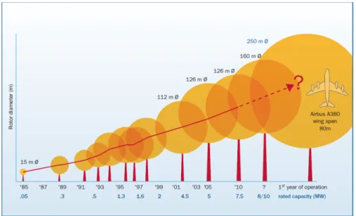
1.1 Wind Turbines rotor size evolution over the increase of rated power. 1
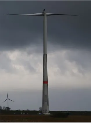
1.2 6MW two-blade wind turbine. . . 2
1.3 Passive load mitigation method: teeter hinge. . . 5
1.4 Modern two blade 2-B 2B6 wind turbine. . . 7
1.5 SkyWind 3.4 MW wind turbine, rotor diameter 107 m. . . 8
1.6 Modern two blade wind turbines: (a) Envision Energy 3.6 MW, (b) Vergnet GEV HP, (c) Windflow 45/500 and (d) Seawind 6.2 MW. . 9
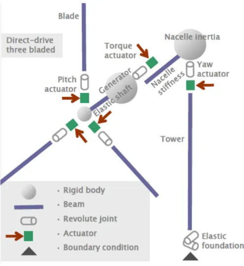
2.1 Topological view of a wind turbine mode il Cp-Lambda . . . 12
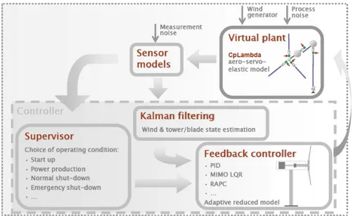
2.2 Control module schematics and its link to the virtual machine . . . 13
2.3 Cp-Lambda curves and regulation trajectory . . . 15
2.4 Region II . . . 16
2.5 Region III . . . 17
2.6 Region IIHalf . . . 18
2.7 Torque over wind speed for a generic wind turbine with IIHalf region 21 2.8 Schematics of a PID+PI controller using an anti-windup system . . 22
2.9 Non-linear collective-only reduced model . . . 23
2.10 LQR with integral state schematics. . . 26
2.11 LQR with integral state augmented system. . . 27
2.12 Cp-λ curves, azimuth angle equals to 0 degrees . . . . 28
2.13 Cp-λ curves, azimuth angle equals to 90 degrees . . . . 28
3.1 Comparison between the different power curves . . . 31
3.2 Pitch weight distribution for the LQR wind scheduling . . . 32
3.3 Torque weight distribution for the LQR wind scheduling . . . 32
3.4 Power mean and standard deviation compared . . . 33
3.5 Torque mean and standard deviation compared . . . 33
3.6 Thrust mean and standard deviation compared . . . 34
3.7 Teeter angle for DLC11 comparison . . . 34
3.8 Blade flapwise-edgewise, ultimate loads . . . 36
3.9 Hub nodding, ultimate loads . . . 37
3.10 Hub yawing, ultimate loads . . . 37
3.11 Tower top Fore-Aft, ultimate loads . . . 38
3.12 Tower top FA-SS, ultimate loads . . . 38
3.13 Tower root Fore-Aft, ultimate loads . . . 39
3.14 Tower root FA-SS, ultimate loads . . . 39
3.15 Teeter angle comparison . . . 40
3.16 Tip displacement comparison . . . 41
3.17 Blade flapwise fatigue loads . . . 42
3.18 Blade flapwise fatigue loads cumulated with Weibull distribution . . 42
3.19 Hub nodding fatigue loads . . . 43
3.20 Hub nodding fatigue loads cumulated with Weibull distribution . . 43
3.21 Hub yawing fatigue loads . . . 44
3.22 Hub yawing fatigue loads cumulated with Weibull distribution . . . 44
3.23 Tower top Fore-Aft fatigue loads . . . 45
3.24 Tower top Fore-Aft fatigue loads cumulated with Weibull distribution 45
3.25 Tower root Fore-Aft fatigue loads . . . 46
List of Tables
2.1 Design load cases utilized. . . 14
3.1 Wind turbine specifics . . . 29
3.2 Ultimate loads for the initial controller . . . 30
3.3 Annual Energy Production due to different control laws . . . 31
4.1 Ultimate loads final comparison and percentage variation . . . 49
4.2 Final comparison of the cumulated DELs . . . 49
4.3 Maximum tip displacement comparison . . . 50
4.4 Aep comparison . . . 50
Sommario
Il lavoro svolto all’interno di questa tesi consiste nel confronto fra tre diversi sistemi di controllo applicati a un aerogeneratore bipala di potenza nominale 10 MW. La macchina è stata progettata con una cerniera di teeter, utilizzata come metodo passivo di alleviazione dei carichi a cui essa è soggetta, e con una torre rigida, aspetto dovuto a elevati carichi a fatica causati dalla risonanza. L’obiettivo è di comparare le differente strategie di controllo col fine di verificare quale abbia il comportamento migliore durante il ciclo operativo della macchina. Particolare attenzione verrà posta nel tentativo di ridurre sia i carichi ultimi, a cui la macchina è soggetta, che i carichi a fatica. Raggiungendo tale risultato, sarà in futuro possibile un re-design dell’aeorgeneratore il cui fine ultimo sia una riduzione del costo dell’energia. La legge di controllo inizialmente presente consiste in un PID affiancato da una tabella usata per la regolazione della coppia in regione IIHalf.
Successivamente verrà testato un controllore PI sulla coppia, in sostituzione della tabella; infine, si applicherà alla macchina un controllore LQR con stato integrale sulla velocità angolare e wind scheduling. A seguito dei risultati ottenuti si faranno considerazioni in merito a quale strategia sia risultata più vantaggiosa in termini di AEP, carichi ultimi e carichi a fatica.
Parole chiave: Aerogeneratore, Bipala, Legge di controllo, Analisi dei carichi,
Analisi a fatica
Abstract
The work within this MSc thesis revolves around the comparison between three different control strategies for a 10 MW two-bladed wind turbine. The machine was originally designed with a built-in teeter hinge, used as a passive load mitigation method, and with a stiff tower, due to the increase in fatigue loads caused by resonance. The aim is to make a comparison between different control strategies in order to verify which one performs in the best way under different operative conditions. The focus will be set on reducing both ultimate loads and fatigue loads. If this effect is achieved, the machine will be able to undergo a new design process whose ultimate outcome might be the the reduction of the Cost of Energy. The starting control law is PID controller using a Look Up Table for handling the region IIHalf of the machine. It will be modified at first with a PID controller acting on
the pitch angle alongside a PI acting on the torque. Lastly, a MIMO LQR with wind scheduling and integral state on the rotor speed will be tried on the machine. After having analyzed the results, it will be discussed which controller performed best from the point of view of AEP, ultimate loads and fatigue loads. Keywords: Wind Turbine, Two-Blade, Control Laws, Loads analysis, Fatigue analysis
Chapter 1
Introduction
The evergrowing need of energy production has always been a paramount issue in Western society. For this reason, countries seek energetic self-sufficience in order to avoid the economic expense of importing either coal or oil.
Within this frame of mind, the importance of relying on alternative sources, especially on wind energy, is clear. The benefits of investing in wind energy are significant. First of all, in a world where the environmental awareness is constantly increasing, renewable sources are required to be exploited as much as possible instead of using polluting ones. Furthermore, the wind resource is definitely more available then the fossil counterpart, allowing several countries to sustain a part of their energetic demand without resolving to importing it. Last, but not least, even though society has been using windmills since ancient times, wind turbines have been developed thoroughly only for some decades; as a consequence, renewable energy manufacturers are still in the process of developing new design strategies in order to increase the efficiency of wind turbines. A desirable goal for innovative design approaches is to raise the Annual Energy Production (AEP) of the turbine while simultaneously reducing the Cost of Energy (CoE) [39].
Figure 1.1: Wind Turbines rotor size evolution over the increase of rated power.
To make possible for this branch of renewable energy to thrive, economics aspects must be carefully considered. In the second half of the 20th century, goverment-funded projects allowed to obtain significant engineering breakthrough concerning wind turbine design; from that point onward, industries tried to make wind energy price competitive against other production methods. To do this, several parameters must be considered in order to evaluate whether the project of a turbine is economically feasible or not. One important aspect is the site where the machine will be built: depending of how windy the location is, the probability distribution function used to describe wind speed on site will be within a wind class, and the wind turbine must be built accordingly. Other important factors to keep in mind during preliminary design are the cost of the land or the restriction due to noise level in densely populated areas, the latter being a significant constraint in recent years. Public acceptance must also be considered: some people find the presence of wind turbines within the natural landscape to be aesthetically displeasing [38].
Figure 1.2: 6MW two-blade wind turbine.
It can be noticed from Figure 1.2 that, over the last few years, industries managed to build increasingly bigger wind turbines. As a consequence, to avoid troublesome noise contraints, as well as due to the lacking of idoneous places on land, the current trend is to build on offshore sites. At first, wind farms have been employed on shallow waters; subsequently, with the advent of multi-megawatt turbines, their construction moved to deeper waters, several kilometers away from the coast.
Due to the rapidly increasing dimension of wind turbines, manufacturing cost is also skyrocketing as well. Thus, solutions are currently being seeked in order to reduce the expenses. A pioneering path is that of two-bladed design: rotor blades of multi-megawatt machines can be more than seventy meters long and are very costly; therefore it is clear that wind power companies will benefit from building one less, both from the manufacturing point of view as well as from the logistic one (i.e. transportation to the site and installation).
However, moving from a three-bladed design to a two-bladed one does not come without several complications. First of all, due to the reduction of the number of blades, the solidity of the rotor decreases accordingly, and with it the obtainable
3
power; as a consequence, solutions such as increasing the blades’ solidity itself must be adopted. Furthermore, due to the rotations being asymmetric several problems linked to fatigue loads arise. Both the moment of inertia variation, which is based on wether the blades are in horizontal or vertical position, and the bending moment acting on the hub, having a frequency value equal to twice the rotational one (2P), lead to higher values in the loads to whom a two-bladed turbine is subjected with respect to a three-bladed one. All of these issues must be kept in mind during the design process.
1.1
Motivation
As it was mentioned before, due the rise of Europe’s interest in renewable and clean source of power, wind turbines are likely to play a critical role on the energy production scenario, and offshore wind farms are being built. Those farms rely mainly on 5-6MW three-bladed wind turbines, and their aim is to make wind power an evergrowing asset among the currently available energy resources. To accomplish this, however, there will be the need of designing bigger machines, and to solve problems related to operating large wind farms (namely of the order of 500-1000 MW) [16].
As a consequence, several matters will have to be addressed due to the problems rising from the upscaling of wind turbines. First of all, the economic perspective must be considered. As multi-megawatt wind turbines increase in size, the manu-facturing cost rises significantly. The need to also overcome other expenses, such as transportation cost, resulted in a recent focus on deeper water offshore plants, in Northern and Southern Europe alike. Another key factor is the mantainance cost of the wind farm. In an attempt to reduce the overall economic weight, some wind power companies are thinking of focusing on two-bladed design instead of a three-bladed design. Doing so would result mainly in a lower manufacturing cost as well as lower maintainance expenses. [25].
There are also several complication arising from the upscaling procedure. It is difficult to estimate correctly the cost of energy derived from wind farm operating with large machines (more than 6MW); this is due to the fact that "ordinary" cost models are based on the fitting of the individual cost of smaller turbines’, such as the 5MW NREL one [11]. Some studies on how to estimate the cost of upscaling have been already done, using appropriate cost models and evaluating whether there is an actual benefit in building larger machines or not. The results showed up that "without additional technology improvements the levelized component cost
increases with turbine size. If new solutions with high fixed cost are introduced, the optimum size (in terms of cost-effectiveness) for components shifts to larger values" [30]. Thus the importance of developing the design procedure for large wind turbines. Another important issue when tackling the task of upscaling is to choose the proper design objective; while smaller turbines design is inherited from the aviation industries, the same design parameters are no longer viable for large, multi-megawatt ones. The latters are in fact to be designed with the aim of minimizing the ratio between the machine operation and maintainance expenditures and its annual energy production. [30] [5].
Even though there will be several advantage concerning the cost reduction of the machine, switching from a three-bladed wind turbine design to a two-bladed one does not comes withouth several drawbacks. The most easily noticed is that the rotor’s solidity will be decreased. As a consequence, the turbine will extract less power from the wind source. A solution could be to increase the solidity of each blade; this way there will be also an increasing of blade stiffness and, as a result, a decrease in the amount of structural material needed [6].
Another major problem is load mitigation. While control technologies for a three-bladed machine are well known nowadays, the same cannot be said for two-three-bladed ones. The dynamic of fatigue loads are more complex, and uneven aerodynamic
1.1. Motivation 5
forces will generated forces that must be absorbed by the turbine structure. To tackle this issue, load reduction techniques must be applied. A first method is to indtroduce a teeter hinge (see Figure 1.3) to connect the rotor to the shaft; this will reduce out-of-plane loads transmission, as the rotor will be free to move in the fore-aft direction. In addition to this, a second path towards load mitigation is to implement a control system able to reduce the loads transmission experienced from the various structural components. Such methods could involve an individual pitch control system, so that cycling pitching will mitigate the periodic sampling on the turbine. Attempts to implement this technique have already been made from a theoretical point of view, via the use of methods such as the multi-blade multi-lag transformation [24]. However, these kind of methods were not taken into consideration during this work since they cannot be easily applied to a design process. Improving the control law acting on the machine is thus a valuable way to improve two-bladed wind turbines performance. [6] [16].
1.2
Scope
The recent trend in the wind energy field is to move toward bigger machines, although the consequences of upscaling upon the manufacturing and operating costs of wind turbines are not fully characterized yet. This is due both to the lack of available data to validate the cost models and the relative novelty of most very-large turbines. Having the same aim in mind, several companies in this industies seem interested in the design of two-bladed wind turbines instead of three-bladed ones; this is because, as the size of these machines increases, the cost of blade manufacturing escalates as well. Apart from reducing the number of blades, different paths can be followed that lead to the same goal of reducing Cost of Energy. One way can be the introduction of passive load mitigation systems, aimed at reducing the fatigue and ultimate loads acting on the machine, and as a consequence allowing a saving on the building cost from the structural point of view. The same results can be reached through a more accurate choice of control laws acting on the system: the use of control strategies which are able to handle critical operative region can result in the machine being subjected to smaller loads throughout its lifecycle. The scope of this MSc is to test different control law for a 10 MW two-blade wind turbine designed with a stiff tower and a teeter hinge for passive load mitigation purpose. The main tool that will be used is the Cp-Lambda code [7]. The software will be thoroughly described in the following Chapter. The focus of this work will be on testing different controllers in order to evaluate their performances from the point of view of ultimate loads and fatigue loads acting on the machine. The first step will be introducing a PI controller on the torque for handling the II.5 region of the machine; this will substitute the Look Up Table previously utilized for the same purpose. Then a model-based control strategy, namely a MIMO LQR with wind scheduling and integral state on the rotor speed, will be tested, in order to see if its performance will be better than the previous control laws.
1.3. State of the Art 7
1.3
State of the Art
Figure 1.4: Modern two blade 2-B 2B6 wind turbine.
Although the history of two-bladed wind turbines design goes back to the first years of the 1940s, the machines of interest for this work are the newest ones; therefore there will be more focus on recent machines rather than on older designs. In particular, several attempts at innovative control designs and loads mitigation techniques will be highlighted; this will be done to show the different challenges that occur when dealing with a two-bladed design instead of a three bladed ones.
After a hiatus in the 1990s, where wind turbine design focused primarily on three-blade wind machine, the increase on offshore wind energy plants reignited interest in two-blade turbines after the 2000s [28] [29]. Technological improvements made it possible to develop a wide variety of wind turbines; this was due to the introduction of control systems, both active and passive, within the wind turbines design. These methods include pitch and yaw control, teetering hub and individual pitch control [26] [6].
In the Netherlands, wind turbine 2B6 was built by 2-B Energy company (Figure
1.4); it was a 6 MW machine featuring a rotor diameter of 140.6 meters. The design included a rigid hub and individual pitchable blades; in addition to this, active yaw damping system was built within the machine. [2]. Van Solingen et al [32] used this turbine to develop a control strategy focused on the IPC. Since the objective of yaw and loads control were conflicting, two different strategies have been used and compared from a controller design point of view. Results showed that the yaw controller design should be carried out in a careful way, since it has a significant impact on the loads acting upon the turbine. It was also noted that the amount of yaw damping provided was a tradeoff choice between blade and tower loads; as a consequence, it is a critical value from the design point of view. Furthermore, the possibility to add yaw damping by IPC meand was demonstrated, with advantages from the point of view of decreasing the tower base torsional moment.
Figure 1.5: SkyWind 3.4 MW wind turbine, rotor diameter 107 m.
In 2016, The German manufacturer Skywind listed on its website a 3.4 MW wind turbine featuring a concrete tower and that can be installed either onshore or offshore (Figure1.5) [31]. On this machine, an innovative load reduction strategy was tried by Luhmann et al. [17]. It consisted in using a flexible connection between the hub mount and the a nacelle carrier. The aim was to assess the consequence that introducing this flexible element might have had on the system dynamics as well as its aeroelastic response to load imbalances. A cardanic spring-damper element is added between the hub and the carrier in order to limit the rotational motion of the joint. A parametric analysis was performed for different values of both stifness and damping parameters; for particular values of the formers, the results showed that the loads on the support structure can be reduced significantly. Using a relatively soft connection (i.e. low stifness) or applying high damping values leads to a reduction of fatigue loads. The downside, however, is the potential risk of exceeding the constructive limits of the turbine.
Envision Energy [9], a Danish company specialized in wind power, developed a 3.6 MW turbine featuring pitchable blade as a load reduction method (Figure 1.6
(a)). Another developer of modern type two-blade wind turbines is SCD-Technology [27]. They build machines for both onshore and offshore usage; the former ones had a rated power in the range of 3-3.5 MW while the latter consisted in two main types: a 6 MW, 140 meters of rotor one with fixed foundations and a 8 MW, 168 meters with floating foundations. All these kinds of machines have a pitch control system; however, none showed a yaw control, being them self-adjusting to the wind direction.
1.3. State of the Art 9
(a) (b)
(c) (d)
Figure 1.6: Modern two blade wind turbines: (a) Envision Energy 3.6 MW, (b) Vergnet GEV HP, (c) Windflow 45/500 and (d) Seawind 6.2 MW.
In France, the company Vergnet Eolien [36] is leader in developing and man-ifacturing medium size wind turbines of about 200 kW of rated power and a 32 meters rotor diamemter. One of their machine, the GEV HP (Figure1.6 (b)), show interesting technological improvements: it is a 1 MW wind turbine with a rotor diameter of 62 meters, showing an innovative teethering hub named "delta-3". This hub significantly decreases load fluctuations due to turbulent winds. Furthermore it features a lowering system wich allows maintainance operations to be done easily.
Moving outside Europe, several interesting two-blade designs can be found. In New Zealand, for example, the Windflow Technology Ltd. [41] manufactured two medium size onshore wind machines, namely the 33/500 and the 45/500 (Figure
1.6 (c)). They both show a teethering hub alongside a pitch control, and have a rated power of 500 kW. The size of their rotors is, as the names suggest, 33 and 45 meters respectively.
Going back to the US, we can delve into the offshore field looking at Seawind Ocean Technology [33] and its 6.2 MW turbine (Figure 1.6 (d)). This machine has a concrete foundation that allows it to operate in water as deep as 50 meters. Its core feature, however, is the laser detector system, capable of spotting either hurricanes or strong gust. This way, the machine will know in advance to point the blade tips along the wind direction. A future developement of this project (which is due to Fall, 2018) is to upscale the turbine up to 10 MW of rated power and 160 meters of rotor size.
Using a two-bladed wind turbine entail several problems with respect to a standard three-bladed configuration. The results of the work of Bergami et al. [3] show the issues arising by moving from a three-bladed design to a two-bladed one, as well as the effect that a teetering hub has on the machine loads. The analysed wind turbine is the DTU 10 MW reference one. To maintain the same solidity of its three-bladed counterpart, the blade chord is increased accordingly. The potential benefit derived from both having a lighter rotor weigth and using less construction material is however counterbalanced by a reduction of the power outcome as well as an increas in load variations. The latters are caused by interaction bewteen tower frequency and a frequency equals to twice the rotational one (2P). To reduce this interaction, a more compliant tower structure could be applied, with the potential drawback of a negative influence on the controller behaviour. A teetering angle was applied during this work in order to reduce loads derived from aerodynamic unbalance. This strategy proved to be very effective, at the expense of a potential reduction of the tower clearance for particular operating conditions.
To conclude, we can observe that several attempts are being performed in order to solve two-bladed issues. Finding a proper solution it is not simple, since different (and often conflicting) factors must be considered, as shown before.
Chapter 2
Methodology
2.1
The Cp-Lambda Code
Cp-Lambda (Code for Performance, Loads and Aeroelasticity by Multi-Body Dynamic Analysis) [7] is a code able to simulate both the static and dynamic behaviour of a wind turbine undergoing either standard or abnormal operating conditions. The multi-body approach means that the code features a library containing a variety of items, both flexible and rigid ones, that can be connected by different kind of constraints (see Figure2.1). Some of the elements included are:
• BEAMS
There is no limitations concerning beams geometry that can be included in the model; furthermore, Cp-Lambda makes it possible to model composite beams. The software is an aeroservoelastic one: as it supports fully populated stiffness matrices, aeroelastic coupling can be taken into account. Reference lines might be curved, since they are obtained by using NURBS (Non Uniform Rational Basis-Splines); they can be also twisted, though.
• JOINTS
All joints contain spring, damper, backlash and friction; in addition to this, they can also be flexible (contact beam-cylindrical, prismatic, screw). The list of joints features cylindrical, prismatic, revolute, spherical, screw and planar ones.
• ACTUATORS
Actuators can be of both first and second order, either linear or rotational. Refined models are available.
• SENSORS AND CONTROL ELEMENTS
The formers are used to measure the system states, while the latter elements read values from a sensor list and apply the changes to either the actuators or to prescribed displacement elements.
Compared to the classic simulation codes, such as FAST [10], focusing just on wind turbines, the major advantage of Cp-Lambda’s multi-body approach is that it
allows to model more complex topologies by assembling simple elements together. As a consequence, it is a more versatile code.
Figure 2.1: Topological view of a wind turbine mode il Cp-Lambda
Having defined all the elements in the library, the structural model is then discretized. Using a finite elements approach, Cp-Lambda will create the mesh and then, given the aerodynamic loads, the machine’s dynamic behaviour will be computed. The output will be fed to the aerodynamic module.
Within the code, the blade-element momentum theory is implemented. The aerodynamic properties of the blades are defined by lifting lines (two-dimensional strip theory), along which the Cl, Cd and Cm values of the airfoils are defined; thus the geometry of the airfoils is not required. On each airstation, the mode computes the relative velocity as well as the attack angle. Thanks to the aerodynamic coefficients table it is possible to obtain the aerodynamics loads acting on the blades; those loads will then be used in the structural module following an iterative process.
Before running the aerodynamic and structural modules, the wind must be modeled. A three-dimensional grid is generated, defining wind properties in a set of points for all the time steps required by the relative simulations. The parameters to be considered during this procedure are the average wind, wind shear, tower shadow and inflow.
2.1. The Cp-Lambda Code 13
Control laws are externally written (see Figure 2.2) in order to be able to use the same control system implementation for both the numerical analysis and experiments; thus it will be possible for the control module to be directly linked to the actual machine.
2.2
Certification Requirements
Operative status DLC Wind Grid loss Safety factor
Power production 1.1 NTM N Normal 1.3 ETM N Normal Power production plus fault 2.1 NTM Y Normal
2.3 EOG Y Abnormal
Parked 6.1 EWM N Normal
6.2 EWM Y Abnormal
Table 2.1: Design load cases utilized.
According to the International Electrotechnical Commission [14] guidelines, a wind turbine must be tested under different design load cases (DLC), each representing either different operative conditions or wind behaviour. Among the numerous scenarios, only the most significant ones have been selected, in order to reduce the required computational time. The complete list of DLCs is shown in Table
2.1. The different design load cases are performed under different wind conditions; the four that are listed in the aforementioned table are: Normal Turbulence Model (NTM), Extreme Turbulence Model (ETM), Extreme Operating Gust (EOG) and
Extreme Wind speed Model (EWM).
In some of those operating conditions, the machine also undergoes a grid loss condition; this can be caused by different factors, losing connection to the electrical network being one of them. This is done to be sure that the machine design will be done considering every possible working condition for the turbine, however unlikely they might be. The last column shows the safety factor corresponding to each DLC; this parameter is applied to ultimate loads for safety measures, as the name suggests. For cases that are more likely to occur, a normal safety factor of 1.35 is used; on the other hand, an abnormal one of 1.10 is considered enough for fringe cases.
When comparing the significant results regarding the machine overall perfor-mance, both utlimate and fatigue loads will be considered. However, while the formers will be evaluated taking into account all the DLCs, the latters will be obtained only from DLC 1.1, as it is the wind turbine’s normal operative conditions.
2.3. Control Laws 15
2.3
Control Laws
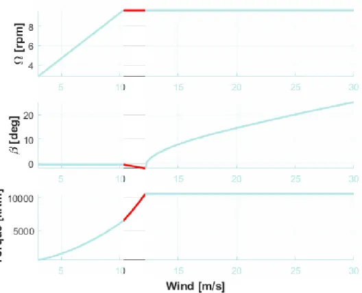
Figure 2.3: Cp-Lambda curves and regulation trajectory
In this work, different control laws will be implemented within the wind turbine, in order to compare their performances and draw several considerations.
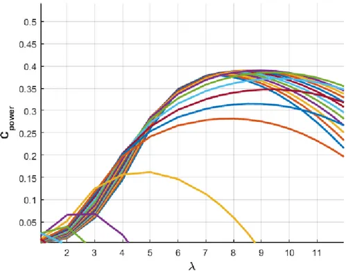
The control parameters are defined starting from the machine’s trajectory regulation. Cp-λ curves like those on Figure 2.3 are obtained for different values of the pitch angle β. Those curves show the relation between the power coefficient of the wind turbine and its Tip Speed Ratio (TSR, often defined with the greek letter λ), for any fixed β. For each pitch angle, it can be found the optimal TSR value, λ∗, and its related optimal Cp, Cp∗. Then the envelope can be obtained by
following the optimal values for each possible pitch angle.
There are three different operating regions for the wind turbine; the regulation strategy has a different behaviour depending on which region is being considered.
2.3.1
Region II
In this region, the aim is to constantly maintain the Tip Speed Ratio equal to its optimal value λ∗, thus having an optimal Cp; maintaining a power coefficient value equal to Cp∗ means maximizing the power output. The pitch angle is maintained constant, equal to otpimal value β∗, while the main control action is that of targeting the desired rotor speed for the actual intensity of the wind. This is obtained mainly by adapting the reacting torque to the fluctuations of the rotor speed. As a consequence, we have β = β∗ λ = λ∗ Cp = Cp∗ Ω(V ) = V λ ∗ R P (V ) = 1 2ρV 3ACp∗ T (V ) = 1 2ρRV 2ACp ∗ λ∗
Where R is the rotor diameter, Ω is the rotor speed, A is the rotor surface, P is the power and T is the Torque. From the equations it can be seen that, for a fixed value of the TSR, the rotor speed is linearly related to the wind speed.
Figure 2.4: Region II
2.3.2
Region III
Once the machine reaches the rated power, it must be controlled in a way that will make it possible to maintain that value. The rotor speed (and, as a consequence, the torque) will reach its rated value of Ω∗ and will be kept constant, meanwhile the pitch angle will be used as the control variable.
β = β(V ) λ = ΩmaxR V Cp(V ) = 2Prated ρV3A Ω(V ) = Ω ∗ P = Prated T = Prated Ω∗
Since now the rotor speed is fixed, from the formulas it can be clearly seen that, as the wind speed will increase, then as a consequence the TSR will decrease in value. As the new aim is have P equals to the rated one, to compensate the power increase due to the rising of wind speed the Cp decreases accordingly. The regulation strategy will follow the envelope of the Cp-λ curvers, moving to a different optimal TSR accordingly to the variation in pitch angle.
2.3. Control Laws 17
Figure 2.5: Region III
2.3.3
Region II
HalfIn wind turbines of noticeable size, an additional constraint is imposed on the maximum tip speed of the rotor blades; this is done to minimize the noise produced by the rotating machine, which can likely reach nuisiance levels. As a consequence, when the machine is being controlled using its rotor speed (i.e. in the region II) and this design contraint is active, Ω must not be allowed to grow over a pre determined limit value. When this limit is reached, the machine will keep a fixed rotor speed Ωmax regardless of the actual value Ω∗. If Ω∗ is lower than the ideal value, this
creates a region where the rotor speed is sub-optimal, thus leading to a certain loss in power which must be suitably minimized.
β(V ) = arg maxβCp(λ(V ), β) λ = Vtip V Cp(V ) = maxβCp(λ(V ), β) Ω(V ) = Ωmax P (V ) = 1 2ρV 3ACp T (V ) = 1 2ρV 2ACp λ
In this transition region that connects region II to region III the control acts on both pitch angle and torque. The power has to reach the rated value in the latter region but the rotor speed must remain fixed; as a consequence, the torque will have to increase. The TSR will be inferior to the rated value and the regulation strategy will move away from the envelope of the optimal condition. To make it possible for
the machine to work at maximum power coefficient, the regulation strategy will move along the Cp-λ curves looking for the pitch value that will correspond to it [4].
2.4. Controllers 19
2.4
Controllers
The behaviour of different controllers utilized in this MSc will be now discussed and analyzed, in order to better explain the final results of this work, showed in the following chapter. The baseline machine utilizes the DTU controller [12] a PID controller acting on the pitch angle, alongside another PID for torque regulation in both the II and IIHalf region; this kind of controller needs additional external
input, namely a table of reference pitch value for different wind speeds, that must be obtained from the machine’s trajectory regulation. The following change was to implement a PID controller that, in order to manage the IIHalf region, uses a PI
controller on the torque, without the need of an external pitch angle table. This has been done to verify wether it allowed a better performance of the machine in that critical region or not. Last but not least, a Multi-Input Multi-Output (MIMO) LQR controller with integral state was tested, moving into a model-based control strategy that could supposedly have yet better performance than the former strategies.
2.4.1
PID on Pitch + LUT on Torque
The PID controller is the most simple to apply to the machine. This is because it just takes into account the rotor speed, not the actual model of the machine. In order to finding the optimal pitch the following formula is used:
βc= Kp(Ω − Ω∗) + Ki
Z t
t−Ti
(Ω − Ω∗)dτ + KdΩ˙
Where K values are the proportional, integral and derivative gain values, re-spectively, and Ω∗ is the desired rotor speed value. This type of controller thus needs the three gains to be set up in such a way to have a quick response without it being too fast nor to risk losing power. As it can be seen, the only sensor needed is the one that measures the wind turbine’s rotor speed; not even the wind value is needed for it to function.
Considering the region II, we previously saw that the formula for computing the torque is:
T = 1
2ρRV
2ACp ∗
λ∗
Remembering the definition of Tip Speed Ration, and substituting V with it, the equation can be manipulated in the following way:
T = 1 2ρRV 2ACp ∗ λ∗ = 1 2ρR 3ACp ∗ λ∗3Ω 2 = KΩ2 = T (Ω)
Thus it can be seen that, being the rated values of both power coefficient and Tip Speed Ratio fixed known values, the only unknown variable, whom the torque depends to, is the rotor speed. This value of K is given by the Look Up Table, giving different values of torque as the rotor speed increases. Within the IIHalf
region, however, this square dependance on Ω no longer applies. This is due to the fact that, as the torque must increase to reach the rated power, the rotor speed must not succeed the Ωmax constraint. The easiest solution to solve this problem
from the control point of view is to make the torque follow a linear behaviour. This is obviously an approximation, since theoretically the torque value should jump right away from the last value of the region II to the rated value, and that is impossible. The main advantage of this method is that the only change that has to be made to the controller is inside the K value within the Look Up Table. The downside, however, is that in that region the machine will not be working in its optimal range anymore.
2.4.2
DTU Controller
The DTU controller is still a PID acting using the pitch angle as a control variable. However, instead of a LUT for managing the regions were the turbine works below rated power (namely regions II and IIHalf), a PID controller acting on
the torque is implemented. For each time step k, whenever the rotor speed Ωk is
far from either its minimum value Ωmin or the rated one Ω∗, both limits for torque
are bound to be:
Tmin,k = Tmax,k = KΩk
On the other hand, when the rotor speed is close to its limits, the torque reference value will be given by a PID accordingly to the error:
eQ,k = Ωk− Ωset,k
Where the set point is the rated speed or the minimum one, depending on the situation.
Due to the torque being bounded, power losses can be minimized acting on the minimum value for the pitch angle βmin,k = βmin(Vk). An external Look Up Table is
used as a reference for minimum values of β at different wind speeds. Thanks to the power error feedback on the pitch PID controller, the reference pitch is maintained at the value βmin.
When the machine operated in region III, the PID on the torque isn’t active anymore, since the torque limits are set by the corresponding control strategy (i.e. constant power or constant torque). The reference value of the pitch angle is given by a combination of PI on the rotor speed as well as both power errors and speed error. The latter is the difference between the generator speed and the rated one; on the other hand, the power errors is obtained by the difference between the rated power and its reference value. As mentioned before, the power error ensures that the pitch angle is kept at its minimum until the rated power is reached. This is due to the fact that both errors contribute to the pitch integral term βI,k.
In case the reference power raises above the rated value, and anti-windup system makes it possible for the controller to quickly increase the pitch angle accordingly. For each time step k, the reference pitch angle is enforced to be:
2.4. Controllers 21
βref,k = max(βmin,k, βP,k+ βD,k+ βI,k)
The integral term for the next step will change only if the reference value of the pitch angle is equal to its minimum limit, since the formula is:
βI,k = βref,k− βP,k− βD,k
Below the rated power value, the rotor speed error is close to zero and therefore the proportional term is negative; as a consequence, the integral term will be positive. In the chance that the value of the reference power get closer to the rated one, the proportional term will be close to zero meanwhile the integral term will still be positive; as a result, the reference pitch angle is going to be still positive and large variations of speed and power will be prevented. The same anti-windup architecture is implemented also on the torque PID controller.
2.4.3
PID on Pitch + PI on Torque
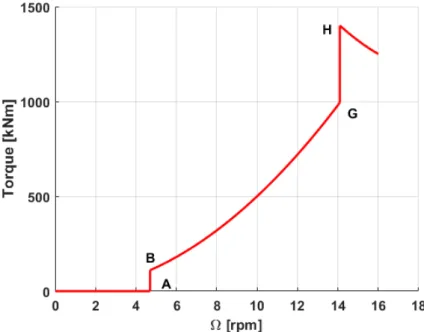
Figure 2.7: Torque over wind speed for a generic wind turbine with IIHalf region
For both region II and II, this kind of controller has the same behaviour of simple PID on pitch + LUT on torque: a PID controller acts as pitch regulator using just the rotor speed as a control variable. As for the IIHalf region, however,
things change: the diagonal ramp approximating the vertical trajectory is no more. Instead, a PI control strategy is applied to track that critical segment of the torque over wind speed graph (line G-H on Figure2.7). Thus, the torque formula in that region becomes:
Tc= Kpt(Ω − Ω∗) + Kit
Z t
t−Ti
(Ω − Ω∗)dτ
Where Kpt and Kit are the PI controller proportional and integral gains,
respec-tively. The most significant consequence, with respect to the former using of a Look Up Table, is that now the control tuning implies the set up of two additional gains related to the IIHalf region. Thus, the aim to optimize the machine’s Annual Energy
Production (AEP) becomes a more daunting task. On the upside, however, the machine will operate at its optimum value, since the former approximated ramp will be substituted with an actual controller instead.
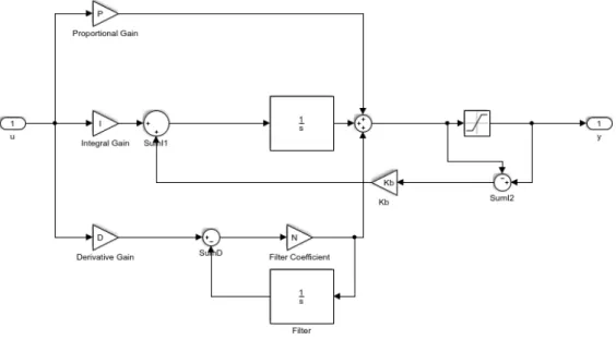
As the control system moves along the curve B-G, the integral part of the PI acting on the torque might grow indefinitely, especially when the machine is subjected to very turbulent winds. To prevent this from happening, an anti-windup system is applied (see Figure 2.8). It consists of an external loop that measures the difference from the torque output and the expected value, namely the B-G curve (used in this case as a lower limit). When this difference is greater than zero, the anti-windup system takes this value, multiplies it with an additional gain
Kb and subtracts it to the integral value in order to prevent the latter to increase
indefinitely.
As the previous one, this controller is not model based, thus it does not take into account any variable besides the rotor speed. When looking for optimal control coefficients, it could be useful to develop a system that takes into account also the optimal wind speed, adjusting the different K values accordingly. This would give information, albeit partial, regarding an additional variable, namely the wind.
Figure 2.8: Schematics of a PID+PI controller using an anti-windup system
2.4.4
Multi-Input Multi-Output LQR
Using a different approach with respect to the previous control laws, the Multi-Input Multi-Output (MIMO) Linear Quadratic Regulator (LQR) is a model based
2.4. Controllers 23
approach. This means that the regulation is based on an actual mathematical reduced model of the machine, with the upside of having access to much more infor-mation than just the rotor speed value. Though not being an exact representation of the machine, the reduced model will allow to properly design the control system in a accurate way.
Figure 2.9: Non-linear collective-only reduced model
The wind turbine reduce model can be seen in Figure 2.9. The dynamics to be considered are:
• The drive-train shaft dynamics. • The elastic tower fore-aft motion. • The blade pitch actuator dynamics. • The electrical generator dynamics.
Thus the states to take into account will be the displacement d, its first order derivative ˙d, the effective pitch angle βe and its first order derivative ˙βe and the
effective electrical torque Tele. The input for this system are, of course, the control
pitch angle βc and the control electrical torque Telc. Writing the equation of motion
(JR+ JG) ˙Ω + Tl(Ω) + Tele − Ta(Ω, βe, Vw− ˙d, Vm) = 0 MTd + C¨ Td + K˙ Td − Fa(Ω, βe, Vw− ˙d, Vm) = 0 ¨ βe+ 2ζω ˙βe+ ω2(βe− βc) = 0 ˙ Tele + 1 τ(Tele − Telc) = 0
Alongside this equation, a slightly different formula for the Tip Speed Ratio must be considererd:
λ = ΩR Vw− ˙d
Where Vw is the sum of the mean wind Vm and the turbulent wind Vt. It must
be noted that, in addition to the rotor itself, the model based approach allows to also manage the tower dynamics, which was not a possible feature using the PID controller.
In the dynamic equations, the aerodynamic force and torque, Fa and Ta appear.
They are computed through the following formulas:
Ta= 1 2ρπR 3CPe(λ, βe, Vm) λ (Vw− ˙d) 2 Fa= 1 2ρπR 2C Fe(λ, βe, Vm)(Vw− ˙d) 2
Where the power coefficient CPe and the thrust coefficient CTe are obtained
off-line using the Cp-Lambda aero-servo-elastic model. Both coefficients depend on the TSR, the pitch angle and the mean wind; the latter is a consequence of taking into account the deformability of both tower and blades under the effect of strong winds.
Re-writing the reduced model in a more compact form, we obtain:
˙
x = Ax + Bu
Where x = (d, ˙d, Ω, βe, ˙βe, Tele) is the state vector and u = (βc, Telc)
T is the
input vector, A and B being known matrices. All non scalar quantities ar expressed in bold in the following equations. The next step is to linearize the model about the desired mean wind values Vm, obtaining:
∆ ˙x = A(Vm)∆x + B(Vm)∆u
∆x = (x − x∗(Vm))
∆u = (u − u∗(Vm))
A(Vm) = A(x∗, u∗, Vm)
2.4. Controllers 25
Where the ∗ apex represent the trim values. The linearization can be done through different approach, such as the analytical method or a numerical one (i.e. Finite differences). A control equation is applied in the form:
(u − u ∗ (Vm)) = −K(Vm)(x − x ∗ (Vm))
Where K is the gain matrix of the control system. The aim of the control system is to minimize a cost function, J, defined as:
J = 1
2
Z ∞
0
(∆xTQ∆x + ∆uTR∆u)dt
It is a constrained optimization problem, the constraint being the linearized reduced model equation. Differently from the PID controller, where the control gains have no physical meaning, the two matrices Q and R represent the importance given to each state and input, respectively. Tuning the controller means defining those weights in such a way to obtain the desired performance from the wind turbine. Using the Lagrange multipliers, represented as λ(t) during the calculation, the equation will become:
J = 1
2
Z ∞
0
(∆xTQ∆x + ∆uTR∆u + λT(∆ ˙x − A∆x − B∆u))dt
From computations derived from the above equation, the following relations are obtained:
Q∆x + ATλ + ˙λ = 0
∆u = −R−1BTλ
The first one is the Lagrange multipliers dynamic equation, while the sec-ond highlights the connection between the system input vector and the λ. The subsequent step is to define the Lagrange multipliers as:
λ = P∆x
Substituting the latter result into the dynamic equation yelds:
˙
P + PA − PBR−1BTP + Q + ATP = 0
This equation is called Riccati Equation. In the steady state case (i.e. as time goes to infinite) the Algebraic Riccati Equation is instead obtained:
The A and B matrices are known from the system formulation, while the Q and R matrices are defined by the weight given to each state and input, respectively. As a consequence, P is the only unknown variable, and solving the problems means finding the proper value of that matrix in order to satisfy the aforementioned constraints. Once P is computed, then the gain matrix K is obtained through the previous relations:
∆u = −R−1BTλ = −R−1BTPx = −Kx
The wind turbine control system will do only the last calculation: the Q and R computation is done off-line, and then the results will be given to the machine which has to solve only the control law.
Wind-scheduled LQR
When doing the aforementioned linearization, the same weights are used for each wind speed. Therefore the input values of both torque and pitch will have the same importance regardless of which wind it is related to. It is possible, though, to select different weights of the inputs for each speed. This allows for the corresponding wind value to have a different focus on torque and pitch with respect to the others. This wind scheduling is not seen by the wind turbine, since the outcome of the calculations is still going to be the Q and R matrices, while the machine will solve only the last equation.
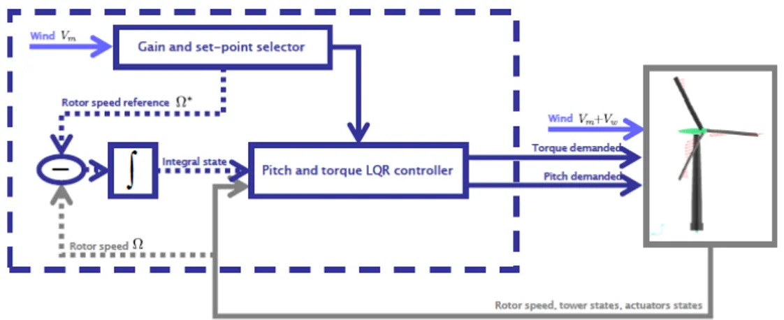
MIMO LQR With Integral State
Figure 2.10: LQR with integral state schematics.
Since the rotor speed is an important state when considering the control system, it is appropriate to further increase its tracking as the machine is operating. This is also a way to compensate eventual errors in rotor speed gain computations that can be caused either to model mismatch issues or a non-optimal weigth choice when tuning the controller. A more accurate tracking of the rotor speed makes possible to correct these errors as well as to obtain a power output closer to the desired set-point.
2.4. Controllers 27
To increase the tracking accuracy a new state is defined, namely an integral state on the rotor speed, so that even if the instantaneous value of this state is not on point, on the long term this error will not be relevant. The controller schematics can be seen on Figure 2.10. The new model will have an augmented state vector
xaug containing the rotor speed integral state in addition to all the former terms.
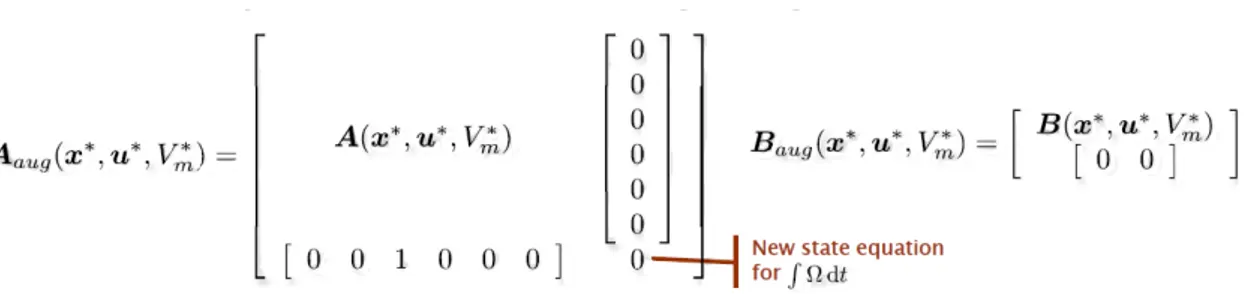
The new augmented system, as can be seen in Figure 2.11, features augmented matrices created using border state-space model matrices.
Figure 2.11: LQR with integral state augmented system.
Reduced model considerations
It is of importance to notice that the rotor of a three-bladed wind turbine has an isotropic behaviour, whereas a two-bladed machine is highly anisotropic. The aerodynamics forces of the model’s equations are computed accordingly to Cp-λ curves that change significantly if the azimuth angle of the blade is modified. This can be easily seen in Figure 2.12and 2.13, showing the Cp-λ diagrams for azimuth angles of 0 and 90 degrees, respectively. While for the 0 degrees case the maximum power coefficient is approximately 0.39 for a Tip Speed Ratio of 8.5, on the other hand for 90 degrees its values is equal to 0.45 and the relative TSR is 8. As a consequence, the reduced models obtained by the two angles are very different, therefore the LQR performance might be better or worse depending on this aspect.
Figure 2.12: Cp-λ curves, azimuth angle equals to 0 degrees
Chapter 3
Results
In this chapter, the results and comparisons between the different control laws and their performances will be showed and discussed. The wind turbine upon which the simulations were run is a two-blade 10 MW machine derived from the DTU 10 MW RWT [1]. The starting machine was previously modified removing a blade and adding a teeter hinge connection to the rotor, as a passive control system aimed at loads mitigation [6].
To avoid resonance problems between the tower and the 2P rotor frequency [3], a stiff tower had to be utilized for this machine, since working into the soft operative range was a difficult, if not impossible, task. The sizing up of the tower was also due to fatigue loads acting on the machine: resonance phenomena, in fact, occurred with this configuration, making a stiffer tower mandatory [6].
The machine specifics and the rated values around which the control was tuned can be seen on Table3.1.
Specifics Values
Class and Category IEC Class 1A Rated Mechanical Power 10.638 [MW] Rotor Diameter 178.3 [m] Hub Height 119 [m] Nacelle Uptilt Angle 5 [deg] Blade Mass 38090 [kg] Tower Mass 1174.2 [tons] Rated Power Coefficient 0.391 [-] Rated Pitch Angle -0.426 [deg] Rated Rotor Speed 9.640 [rpm] Rated Torque 10.538 [MNm]
Table 3.1: Wind turbine specifics
The starting controller is the original DTU one [8]. It consists in a PID acting on the pitch angle plus a PID for torque regulation, alongside an external Look UP Table used for maintain a minimum value of the pitch angle in region II.
It will be compared with two controllers: a combined PID on pitch plus PI on the torque, and a MIMO LQR with wind scheduling and rotor speed integral state.
Load Corresponding DLC Blade Flapwise-Edgewise DLC13-13ms
Hub Maximum Nodding Moment DLC13-17ms Hub Maximum Yawing Moment DLC13-25ms
Tower Top Fore-Aft Maximum DLC61IDT-YMdeg8a Tower Top Fore-Aft Minimum DLC23-vr+2b
Tower Root Fore-Aft Maximum DLC11-25ms Tower Root Fore-Aft Minimum DLC23-vr+2b Tower Top FA-SS DLC13-23ms Tower Root Fa-SS DLC13-25ms
Table 3.2: Ultimate loads for the initial controller
Although the machine has been tested for different DLCs, the comparison of the obtained results will be done focusing on two specific design load cases (DLCs), namely DLC11 and DLC13; this is because the MSc subject are the control laws, and for some DLCs such as the 62, where a grid loss occurs, the controller won’t be able to operate. On DLC11 and DLC13, which represent normal turbulence model and extreme turbulence model conditions respectively, the control system works properly and its performance can be therefore evaluated. Analyzing the DLC11 load values is of use for showing the behaviour of the different controllers during the standard operative condition of the machine. As it can be seen by Table 3.2, showing the ultimate loads (with the relative Safety Factor applied) of the starting machine, whenever the highest values are not caused by a DLC without an active controller (i.e. DLC61 or DLC62), they instead mainly occur during DLC13.
3.1. General Results 31
3.1
General Results
Figure 3.1: Comparison between the different power curves
The first comparison will be done considering the different power curves obtained by using the three controllers. This power curves are based on the data from the DLC11, which is the normal operative condition for the wind turbine. As it can be seen from Figure3.1, both the PID+PI and the LQR are capable of generating a greater electrical power with respect to the DTU controller. As a consequence, the Annual Energy Production (AEP) of the formers will be greater than the latter’s, as shown in Table3.3:
Comparing the above values, it can be seen that using a PID+PI controller allows the power production to increase of approximately 1.8% with respect to the DTU controller, meanwhile the LQR controller performance improves this values of a quantity which is slightly more than 1.6%.
Controller AEP [GWh/y] Variation [%]
DTU 44.67
-PID + PI 45.50 +1.85 LQR 45.40 +1.63
Table 3.3: Annual Energy Production due to different control laws
From Figure 3.1 it can be noticed that the LQR higher production happens around a wind of 11 m/s. Since the Weibull greatest values for this machine are around that speed, this implies that from a CoE perspective the LQR controller will yield better results with respect to the starting DTU one or the applied PID+PI. The downside, however, is that in that region the wind turbine will experience both ultimate and fatigue loads of bigger magnitude.
For a wind speed of 13 m/s, the LQR controller has a smaller power production. This is caused by the increased weight acting on that particular speed, as it can be seen fron Figure 3.2. The higher weight has been done in order to reduce the loads experienced by the machine for that particular value of the wind. Figure 3.3 shows the weight scheduling for the torque, instead.
Figure 3.2: Pitch weight distribution for the LQR wind scheduling
3.1. General Results 33
Figure 3.4: Power mean and standard deviation compared
Figure 3.5: Torque mean and standard deviation compared
Figure 3.4 shows the power mean and standard variation for different wind speeds. At the 11 m/s value the LQR controller features a high standard deviation with respect to the others. This increase can be also noticed in Figure 3.5, showing how the torque mean and standard deviation changes for the different speeds. The increase in power production is therefore at the expenses of both ultimate and fatigue loads experienced by the machine.
Figure 3.6: Thrust mean and standard deviation compared
The increase in torque is the reason why the power outcome of the PID+PI, and the LQR as well, is greater than the starting controller. The thrust also shows an increase, as it can be noticed by looking at Figure 3.6. The same considerations that were done for both power and torque can be done for the thrust as well: it is clear how around 11 m/s the LQR machine will experience greater loads with respect to the ones of the DTU one.
3.1. General Results 35
Finally, a comparison on the teeter hinge angle is also done, in order to evaluate how, during standard operating conditions, its maximum and minimum values over various wind speeds will differ when the machine follows one control law over another. Looking at Figure 3.7, it can be seen that, among the different control systems, the LQR has the overall better performance, even though its values are very similar to the DTU ones. The PID+PI, on the other hand, shows an increase of 1.5 degrees in both the positive (away from the machine) and negative (toward the machine) direction for a wind speed of 13 m/s. Furthermore, its performance is also worse than the other two controllers for the highest wind speeds.
3.2
Ultimate Loads Results
When trying to evaluate and compare the performance of different control systems, it is important to analyze the ultimate loads to which the wind turbine is subjected. If those loads are smaller compared to the ones experienced by the reference turbine, then it means that the controller is working in a more efficient way with respect to the others.
The following Figures, from 3.8 to 3.14, show the results obtained from the ultimate loads analysis for the three different control strategies.
Figure 3.8: Blade flapwise-edgewise, ultimate loads
For the blades, the combined flapwise-edgewise moment has been analyzed. Since it is a comparison of ultimate loads, for each wind speed the greatest values between the two blades has been used. As it can be easily seen from Figure3.8, the LQR controller experiences higher loads overall. This is particularly true around the 13 m/s wind value, when there is an increase of about 8% with respect to the reference controller. The PID+PI controller, on the other hand, yields better results overall; however, its ultimate load is basically equal to the DTU one’s.
3.2. Ultimate Loads Results 37
Figure 3.9: Hub nodding, ultimate loads
Figure 3.10: Hub yawing, ultimate loads
Figures 3.9and3.10show the hub nodding and yawing moments ultimate loads, respectively. From both moments’ perspective, the maximum values are similar one to another, meanwhile PID+PI shows minimum loads of greater magnitude.
Figure 3.11: Tower top Fore-Aft, ultimate loads
It can be seen from Figure 3.11 that, although the LQR is subjected to greater loads around 11 m/s, its maxmimum value is almost equal to the DTU one. The latter has though a worse behaviour when comparing the minimum values.
Figure 3.12: Tower top FA-SS, ultimate loads
Figure3.12shows the comparison between the blades combined moment. Despite reaching a peak value for a wind speed of 13 m/s, the LQR yields extremely good results with respect to the reference controller.
3.2. Ultimate Loads Results 39
Figure 3.13: Tower root Fore-Aft, ultimate loads
Figure 3.14: Tower root FA-SS, ultimate loads
From a tower root FA perspective, the LQR controller shows its advantages. Looking at Figure3.13 we can see that the maximum loads are smaller than the reference one and the minimum, even though a peak is present, is still smaller than both the DTU and PID+PI ones. This is likely due to the weight given to the tower state when computing the matrices used by the LQR controller; the model-based strategy was able to better control the tower.
Looking at the combined FA-SS moment of the tower root (Figure 3.14), the LQR advantages are highlighted even more. Having a decrease in ultimate loads of this magnitude could likely result in a greater performance of the machine from the design perspective, making it possible to have a lighter tower and, eventually, decreasing the Cost of Energy of the wind turbine.
An analysis on the teeter angle, like the one done for DLC11, was performed for this DLC too. The results are shown in Figure3.15. All three controllers shows the same behaviour when compared, with only small differences from one to another. Another parameter that must be kept into consideration during the design process of the machine is the tip displacement. It is in fact of paramount importance that this value is smaller in order not to have a worse clearance between the blades and the tower. Since this wind turbine features a teeter hinge, the tower/blade clearance acts as a contraint [6]. As a consequence, the spar caps thickness will have to be increased, with several complications from the manufacturing point of view. If the tip displacement value is decreased, the contraint will be easily satisfied, without undergoing severe structural modifications.
As it can be seen from Figure 3.16, the machine upon which this thesis LQR controller has been applied shows an increase in the maximum tip displacement value of about 9%. This higher displacement is caused by the flapping moment of the LQR machine being greater than the reference one, due to the increase in power production. On the other hand, however, the machine which uses the PID+PI control law show an overall smaller tip displacement value. This is likely going to result in a reduction of the tower/blade clearance contraint, with is definitely beneficial to the blade design.
3.2. Ultimate Loads Results 41
3.3
Fatigue Load Results
This final section will show the results linked to the fatigue loads to which the wind turbine will be subjected during its lifecycle. The analysis is done considering the DLC11, according to the International Electrotechnical Commission requirements [14]. For each load that has been taken into consideration, two Figures are present. The first one shows the Damage Equivalent Loads (DEL) comparison for different wind speeds, meanwhile the second one displays the value of the DELs cumulated with the Weibull wind distribuction.
Figure 3.17: Blade flapwise fatigue loads
3.3. Fatigue Load Results 43
First, the blade flapwise moment will be considered. As foretold by the analysis in the previous Section, Figure3.17 shows that for wind speeds around 11 m/s the LQR controller is subjected to greater loads with respect to the other two. This can also be seen by Figure3.18, where the cumulated DELs of this controller are far greater than the other two, with an increase of approximately 50% with respect to the reference controller.
Figure 3.19: Hub nodding fatigue loads
Looking at the hub nodding moment, Figure3.19 shows how the loads of the PID+PI controller are overall greater than the other two. The LQR has a similar behaviour to that of the reference DTU system, apart from the 11 m/s region. The peak present in the Figure is caused by that specific wind speed simulation being harshest than the average. Since the Weibull wind distribution is centered around that value, the cumulated DELs of the LQR will be slightly higher than the other ones, as it can be seen from Figure 3.20.
Figure 3.21: Hub yawing fatigue loads
3.3. Fatigue Load Results 45
Analyzing the hub yawing moment, the PID+PI controller features a worse performance compared to the other two, as it shown in Figure 3.21. Both the DTU and the LQR experience approximately the same values, with the latter being slightly worse (as it can also be observed by the cumulated DELs on Figure 3.22).
Figure 3.23: Tower top Fore-Aft fatigue loads
The overall FA fatigue loads experienced by the tower top are lower with respect to the other control systems that have been tested, as it can be noticed from Figure
3.23. However, the anomalous peak around the wind speed of 11 m/s is responsible for a highest value of the cumulated DELs, due to the fact that the Weibull greatest values are around that region. As explained when the nodding fatigue loads were discussed before, the bad turbulence seed is likely responsible for this behaviour. The consequence of this increase is shown in Figure 3.24, where the cumulated DELs are higher than the reference ones.
Figure 3.25: Tower root Fore-Aft fatigue loads
3.3. Fatigue Load Results 47
The last Figures that are going to be discussed will show the benefits that a model-based controller has with respect to controllers that don’t take into consideration the tower dynamics. From Figure3.25, showing the tower root FA Damage Equivalent Loads, it can be seen that the LQR is subjected to much smaller loads with respect to the reference controller. Looking at Figure 3.26, a decrease of about 23% of the cumulated DELs can be noticed. This is of great importance from a design perspective: as the tower experiences loads of smaller magnitude, its stiffness could be lowered. As a consequence, less material will be required and the Cost of Energy will be likely lowered.
Chapter 4
Conclusions
After having thoroughly discussed the results showed in the previous Chapter, several considerations can be made. First of all, it is important to notice that, since a re-design of the machine has not been done yet, the obtained data can only allow us to make educated guesses regarding whether the CoE will actually be better of worse when applying the different control systems that have been tested.
Moment DTU [kNm] PID+PI [kNm] [%] LQR [kNm] [%] Blade F-E 71040 71130 +0.13 76650 +7.90 Hub Nodding Max 14780 14800 +0.14 14770 +0.07 Hub Yawing Max 13320 14190 +6.53 13270 +0.34 TT F-A Max 14270 15380 +7.78 14670 +2.80 TT F-A Min -13950 -13260 -0.49 -11070 -2.06 TR F-A Max 535500 499400 -0.07 459300 -0.14 TR F-A Min -320800 -303800 -0.05 -272400 -0.15 TT FA-SS 24000 24390 +1.63 21940 -8.59 TR Fa-SS 551600 545100 -0.01 451300 -0.18
Table 4.1: Ultimate loads final comparison and percentage variation
Moment DTU [kNm] PID+PI [kNm] [%] LQR [kNm] [%] Blade Flapwise 30710 31130 +1.37 46320 +50.83 Hub Nodding 7726 8243 +6.69 8086 +4.66 Hub Yawing 7779 8588 +10.40 7928 +1.92 TT F-A 10690 11160 +4.40 10850 +1.50 TR F-A 320800 337600 +5.24 248300 -22.60
Table 4.2: Final comparison of the cumulated DELs