JOB RECOMMENDATION BASED ON DEEP LEARNING METHODS FOR NATURAL LANGUAGE PROCESSING
Project in
Text mining
Rapporteur
Prof. Gianluca Moro
Presented by
Lorenzo Valgimigli
Third Deegre Session
Accademic year 2018-2019
1.3.1 Collaborative Filtering . . . 8
1.3.2 Content-Based Filtering . . . 8
1.4 This project . . . 8
2 Domain of the project 11 2.1 Job Recommendation System . . . 11
2.2 LinkedIn: an example . . . 13 2.3 The data . . . 15 2.3.1 window_dates.tsv . . . 17 2.3.2 users.tsv . . . 17 2.3.3 user_history.tsv . . . 18 2.3.4 jobs.tsv . . . 19 2.3.5 apps.tsv . . . 19 2.3.6 Other files . . . 19
2.4 Contribution of this work . . . 20
3 Available Technologies 21 3.1 Attention Mechanism . . . 21 3.1.1 First implementation . . . 21 3.1.2 Multi-Dimensional Attention . . . 22 3.1.3 Self Attention . . . 23 3.1.4 Conclusion . . . 23
3.2 Flair and Contextual String Embedding . . . 24
3.2.1 Experiments and Results . . . 24
3.2.2 Model . . . 25
3.2.3 Contextual Word Embedding Extraction . . . 26
3.2.4 How to use . . . 27
3.3 ELMo - Embeddings for Language Models . . . 27
3.3.1 Overview . . . 27 3.3.2 Model . . . 28 3.3.3 Performances of ELMo . . . 30 3.3.4 How to use . . . 31 3.4 Transformers . . . 32 3.4.1 Overview . . . 32 3.4.2 Model . . . 32
3.4.3 Attention Mechanism in Transformer . . . 33
3.4.4 Multi-Head Attention . . . 35
3.4.5 Feed Forward Neural Network . . . 35
3.4.6 Input and Output . . . 36
3.4.7 How to use . . . 37
3.5 Bidirectional Encoder Representation from Transformer . . . 37
3.5.1 Overview . . . 37
3.5.2 BERT Performance . . . 37
3.5.3 Model . . . 38
3.5.4 Inputs and Outputs . . . 39
3.5.5 BERT Framework . . . 39
3.5.6 How to use . . . 41
3.6 ROBERTA . . . 41
3.6.1 Overview . . . 41
3.6.2 ROBERTA Performances . . . 42
3.6.3 Differences from BERT . . . 43
3.6.4 How to use . . . 44 3.7 Sentence BERT . . . 44 3.7.1 Sentece-Bert Results . . . 45 3.7.2 Model . . . 46 3.7.3 How to use . . . 47 3.8 SHA-RNN Model . . . 47
3.8.1 The sha-rnn model . . . 49
3.8.2 Model results . . . 49
4 Experiments and Results 51 4.1 Development Environment . . . 51
4.1.1 Server . . . 51
4.1.2 Google Colaboratory . . . 52
4.1.3 Python and Frameworks . . . 53
5.1 Last Job Prediction using Job Embeddings . . . 74 5.2 Possible solutions and future works . . . 77
Conclusions and future prospects 81
Thanksgivings 83
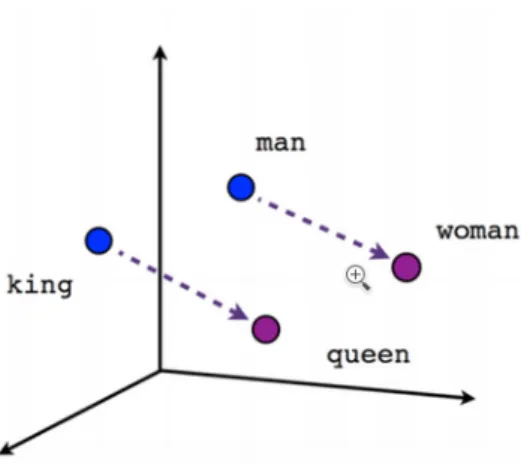
1.1 Vector space representations. In the figure is possible to see how the relationships between words are contained within the
boundaries of this space . . . 4
1.2 Deep Neural Network overview . . . 5
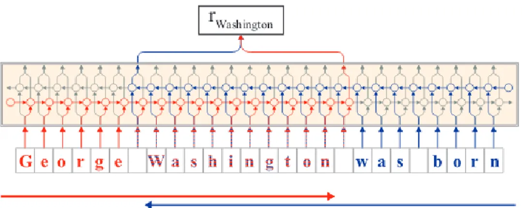
1.3 Intuitive representation of a model that extracts contextual word embeddings from a sentence. Figure from Contextual String Embeddings Paper . . . 6
1.4 Picture from paper Deep Neural Networks for YouTube Recom-mendations[1]. High level representation of the Neural Networks used by You Tube to recommend videos . . . 7
2.1 Recommendations on Amazon . . . 12
2.2 Overview of the LinkedIn recommendation system . . . 14
2.3 Abstract overview of LinkedIn Internal structure for Recruiter system . . . 15
2.4 Overview of the time windows from which data has been taken. 16 2.5 Users table view using Pandas . . . 17
2.6 user_history table view using Pandas . . . 18
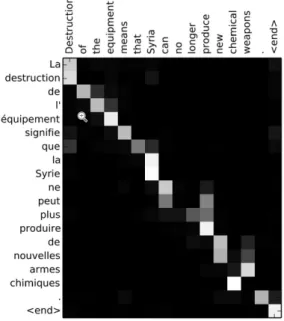
3.1 Graphical representation of attention during translation . . . 22
3.2 Results obtained by using Contextual String Embeddings . . . . 25
3.3 Bidirection LSTM Neural Network . . . 26
3.4 LSTM Layers in ELMo Model . . . 28
3.5 Character-Level CNN used in a lot of models including ELMo. Picture from paper [2] . . . 29
3.6 Highway model. Picture from paper [3] . . . 31
3.7 Encoder-Decoder Architecture of Transformer . . . 33
3.8 Model Architecture of Transformer . . . 34
3.9 Multi-Head Attention . . . 36
3.10 Accuracy for GLUE Task. Picture took from Bert Paper[4] . . . 38
3.11 Bert Model. Picture from Bert Paper[4] . . . 40
3.12 Bert Inputs. Picture took from Bert Paper[4] . . . 41
3.13 GLUE Results for ROBERTA model . . . 42
4.3 Model results tested by using unbalanced datasets . . . 68 4.4 Metrics variation using different split points . . . 69 4.5 Results of the model in last job classification task using
unbal-anced datasets . . . 71 5.1 Keras representation of the model used for job prediction . . . . 76 5.2 Idea for future models for job prevision . . . 79
personal skills but hard to solve problems still exist.
Today, different from the past, we have more tools and more experience to handle such problems and to try to find solutions. One of the most important tools is the computer that has lead us to new solutions and new ways to approach them. The computer has worked fine to face problems which can be rigorous and formally described and for years it has been used to handle these kinds of tasks. However, there are problems which humans can face more or less easily but they can’t be described using rigorous ways. Let’s think, for examples of a man or woman’s face and the goal is to guess if it is smiling or not. This task is incredibly easy for anyone, but it is impossible to describe with some rigorousness. For the human mind it is simple to face those kind of problems, but for a such schematics technology as computers it is impossible. To face them Artificial Neural Networks were born. ANNs are inspired to simulate the human brain and how it works. Indeed, they use as basic unit the Neuron that, like in the brain, is linked to more neurons and receives inputs from other neurons. Another similarity between the human mind and ANN is that both learn from experience but in the first case the experiences are limited and it must learn fast from them. The second case is different in the fact that it can live a lot of experiences in a few seconds. This makes the ANN very powerful and, for some tasks, they surpass humans by reaching better results. From the first promising results Neural Networks has been deployed in many fields: Natural Language Understanding, Events Prevision, Medical Diagnostic System, Products Recommendations and so on.
To face more complex problems Artificial Neural Networks has been modified
by adding inner Neuron Layers to let them model those problems better and better. These modified artificial neural networks are called Deep Neural Networks and, nowadays, they represent a very promising solution for tasks that before were impossible to solve.
1.1
Natural Language Processing
Natural Language Processing is the point where the linguistic field and computer science come together. It concerns all methods, algorithms and tools used by software to process and extract information from human language data. This field includes different tasks as Natural Language Understanding, Speech Recognitionand Natural Language Generation.
For humans understanding their own language is easy and natural, but it is a very hard task for a computer that doesn’t have the ability to deeply understand the semantic of a word. In the human mind exists a special dictionary that links a word to its meaning composed by experiences and sensations. If we read the word ice-cream we get access to a lot of personal information like last time we tasted it or our favourite flavours or ice-cream shop and all of these well define the concept of ice-cream. But computers don’t have such a pool of experiences and this in not the only problem they face. In fact, this field raises other issues:
• Syntax. Syntax structure differs from language to language
• Polysemy. Words can have different meaning according to their usage. • Synonymy. Different words have the same meaning.
• Irony. Sentences written to have a meaning that has to be extracted form the sentence indirectly.
• Orthographic errors. If sentences are hand-written they can contain errors to be corrected.
• Abbreviations or Special Symbols as the emojis. If the aims are tweets abbreviations and special symbols are very common and they have important meaning within the phrase.
To handle all of these problems data preprocessing is a common way to proceed. This phase is composed by well-known steps which aim to clean the text, remove synonymy and errors. These steps can vary from task to task but the most common ones are:
come before the target word and the ones that follow it. To better understand this concept it necessary to define the Context of a word Cwk as the set of the
N words before wk and the M words after.
Cwk = [wk−n, . . . , wk−1, wk+1, . . . , wk+m]
In this way for each word (or token) it’s possible to create a context and then join the contexts of the same tokens which have more recurrences and lastly list those tokens which appear several times. For each word, looking at its context, a list of features can be created using the frequencies of the presence of other words in its context. In this way two words could have a relationship if they share the same or similar context. For example the word ice-cream and the word cold appear to be related in some way because the second is often in the context of the first. This leads computer to create relationships between words and these relationships are the keys to understand the meaning of them.
1.1.1
Word Embeddings
Using this context is also possible, for each word, to create a vector of features composed by real numbers that describes the word itself. This vector is called Word Embeddings and maps the word into a vector space. An intuitive way to create such a vector could be by using a matrix with words in rows and columns. Cell cij contains a natural number that indicates how
many times the word in the column wj appears in the context of the word in the row wi. This kind of matrix is known as Co-occurrence Matrix. In this way for each word in the dataset it possible to create a high dimensional vector that brings information about relationships with other words. At this point, using some advanced techniques as Singular Value Decomposition each vector is mapped to another vector with less features but bringing under light relationships between words (Latent Semantic Analysis). This phase is called Dimensionality reduction and aims to create a vector space where
Figure 1.1: Vector space representations. In the figure is possible to see how the relationships between words are contained within the boundaries of this space
similar words are put close together while different words are placed at some distance. A graphical view of this concept can be found at figure 1.1.
The above explained process is just the basic concept behind the algorithms used in Natural Language Understanding tasks. It is just an intuition of a more complex word, that is the ground on which, works by many researchers has been built. One of this work highlights the importance of studying the frequency of the term in a document in relation to the frequency of that term in the whole corpus [5]. The study of that frequency is fundamental aspect for the Word Embedding creation.
Word Embeddings are the key to solving NLP problems and to create good ones is still an on going task and a lot of techniques have been created to further improve them.
1.2
Deep Neural Network in NLP
In today’s Deep Neural Network era a lot of old techniques have become useless. The Deep Neural Networks bring with them some advantages which make these new models the most favored in many fields of data science. First of all, they don’t need a strong formalism to describe a problem but a lot of examples (x, y) where x is the input of the net and y is the desired output to train the network. Thanks to the new technologies and the coming of big data, Deep Neural Networks achieved exactly what they wanted and they were
Figure 1.2: Deep Neural Network overview
able to expand limitlessly, leading research into unexplored territory. Today they are used to reach state of the art performance, growing day by day, ever improving their results. They are also used in concrete fields like market. One example is the work done by Professor Gianluca Moro regarding how to predict the stock market Dow Jones Index using Tweets [6].
For each data science field a specific Neural Network exists as Recurrent Neural Networkfor data represented by sequence like sentences or Convo-lutional Neural Network for matrices of data and they are widely used in Imagine Processing and so on. The following paragraph will try to explain how deep neural network changed the NLP field.
1.2.1
New Word Embeddings
The basic and most important element for each Natural Language Processing task is word representation in a vector space that shows the relationships between words. This representation is called Word Embedding and the creation of this is a very well studied topic by lot of researchers.
A good way to generate these vectors comes from Deep Neural Networks. The main ingredient to generate them is the Context of a word Cw0 so Deep
Figure 1.3: Intuitive representation of a model that extracts contextual word embeddings from a sentence. Figure from Contextual String Embeddings Paper
[7]
context. For example, masking a word in a sentence and the model has to read the words prior to it and after it and then generate a probability distribution over the dictionary to guess the masked word. Using a large dataset (more than 100 GB) and a lot of training time the model can achieve very good results. This kind of approach forces model to learn relationships between words, to guess which words are nearer to others and how often they occur, but without creating any explicit data structure with this information. In this way, the network learns internally how to model the language. As we know, Deep Neural Networks are by definition, Multi-layered Neural Networks and each layer has a hidden state composed by the state of each neurons. Using these hidden states, which somehow contain what model learned about the language, it is possible to create vectors to use as word embeddings. This is the basic idea on how to use Deep Neural Networks to generate word embeddings but each implementation brings differences and variations which need to be studied.
1.2.2
Contextual Word Embeddings
Using the previously explained approach, the model can read the words prior to the target word and the ones after it and therefore generate a probability distribution over the entire dictionary according to what it has seen.
Let’s define X0:T = (x0, x1, . . . , xT) the language dictionary, wj the masked
word and Cj = (w0, . . . , wj−1) ∪ (wj+1, . . . , wn) its context. So the model tries
to predict the right probability distribution over X0:T.
Figure 1.4: Picture from paper Deep Neural Networks for YouTube Recommen-dations[1]. High level representation of the Neural Networks used by You Tube
to recommend videos
From this description it’s easy to see that the context heavily influences the result of the model. This means that the same word in a different sentence, generates different word embeddings. Using old approaches each word was mapped to a unique vector. With this new technique, however, each word gets a vector strongly correlated to the context and such vectors are called Contextual Word Embeddings. This allows Deep Neural Networks to create better embeddings and reach a new state of the art performance in this field.
1.3
Recommendation Systems
A Recommendation System or Recommender System is a technology that seeks to predict the preference a user would give to an item in the system. For example You Tube Recommendation System [1] is a Neural Network model that tries to predict the favourite videos in the corpus for each user. Improving and deploying recommendation systems are often the main objectives of global companies such as Amazon, Netflix, . . . . It’s a fundamental solution to enhance the user’s experience especially when considering the number of available items grows day by day and for this reason much research and study goes into this field.
1.3.1
Collaborative Filtering
There are two main approaches for the design of a recommendation system: Collaborative[8], Content-Base. In the first case the idea behind it is: two users with similar histories will probably make similar decisions. In this system the user is defined by a series of items e0, e1, . . . , en ∈ E that is to say that
the collection of the previously selected items like videos viewed on You Tube, films watched on Netflix or items purchased on Amazon. If two users have a similar items history, this approach assumes that if item ek will be the next
choise for the first user it will probably be the next choise even for the second user. Matching user items histories the system tries to suggest items with the highest probability of being selected.
1.3.2
Content-Based Filtering
The second approach is based on the description of the item to profile the user preferences. The idea behind it is: the user that has been using the system to buy food and not electronic devices will probably keep doing so in the future. The system will then recommend pizzas rather than smart phones. Also in this case the user is defined by items he previously selected. The model, using these items and the correlating data, tries to create a User-specific Classifier that has to determine whether for each item the user will like it or not. Usually, Recommendation Systems incorporate both of these approaches to achieve the best results[9].
1.4
This project
The goal of this project is to test new technologies as Deep Neural Networks tries to manage problems that classic machine learning algorithms can’t. One of these problems is how to interpret textual data, maybe hand-written, in tasks which aren’t NLP tasks. In particular this work focuses on job recommendation systems where data is not well structured and most of them are hand written by users. In fact, the entire job history is written by each users using his terminology, his descriptions, his detail level, . . . . It can be seen immediately this kind of approach brings a lot of problems:
• Two different jobs can be addressed with the same name. For example a medical assistant or a university professor assistant can be referred using just Assistant but they are very different in particular if the system has to model concepts such as Careers.
those where there is less.
If the goal is to create a model capable to work with this data it is necessary that it can read and understand the sequence of the jobs in a job history. It has to model complex data and work with them. The idea behind this project is to create a system that takes the job history and perhaps some further information about the user and therefore predict the last job of this user. It’s impossible know which is the best job for each user so this project is based on this assertion: the last job of a user was one of the best jobs for him before doing it. Let’s define user u as a list of jobs that he did until time t: u0 =< j0, j1, ..., jn>. So
at the given time t − 1 user is u0 =< j0, j1, ..., jn−1 >. In this case it is possible
to assume that the job jn is one of the best jobs for him because it is the one he
did next. However, guessing the last job is one of the many possibilities: in fact the data also contains job posting and job applications for each user and other information such as level of education, time, location, . . . . All of them compose a variegate picture that brings possibilities and problems. So the question still remains: can Deep Neural Networks make use of these opportunities by overcoming problems?
big companies with thousand of employs know well. Today, part of this work relies on personal specialized in finding the best workers in the market, meeting them and selecting a few of them according to little information. This is a very expansive mechanism that doesn’t guarantee the best results. Therefore one question arises: how new Deep Neural Networks Technologies can be applied to this field and what results they can achieve?
2.1
Job Recommendation System
The efficiency of the Artificial Neural Networks and the Machine Learning Models in Recommendation Field is not deniable. Today many systems relies on this kind of technology to improve the User Experience on one side and to optimize the server computational cost on the other. People interact with this system every day even without knowing it. It is enough to think about Amazon.com Recommendation System that uses a Item based collaborative filtering[10] to recommend items to each user according to his past history. Similar examples can be found everywhere in the web, but all of those systems use well structured data which have a very accessible and explicit information. Automatize these kinds of tasks has been a target for many researchers for years. Job seeking was tricky, tedious and time consuming process because people looking for new position had to collect information from many different sources. To automatize this processJob Recommendataion systems were proposed. They have been used and improved year after year with the best machine learning
Figure 2.1: Recommendations on Amazon algorithms [11].
But now, the question is how Deep Neural Networks can be applied in Job Recommendation tasks even if data are unstructured. First of all it is useful, in order to understand the problem, to formally describe the task. Let’s define a worker wk as a user uk with all information about his working history. This
information can vary from dataset to dataset but they often are:
• Jobs History. This is probably the most important information about the user because it contains all jobs done by the user. Sometimes this job history comes with other useful information for each job like salary, duration, rating, . . .
• Education Level. This information allows the system to better classify the user. Often it contains information as final vote, graduation, extra experiences, . . . .
• User’s preferences. The user can indicate some preference on which field he would like to work. Sometime, this information extrapolated by using user’s researches.
• User’s skills. User can select or write some skills he thinks to have. This information can be useful to pair the user with a job that requires explicitly or implicitly some skills.
Now let’s define a company ck as the element in the system that produces job
• Hard and soft skills. Job posting can indicate which skills are required (Hard Skills) and which are welcome (Soft Skill). This information can
help the system to find the right worker for this job posting.
• Experience required. This information tells how many years and which kind of experience the candidate should have. It can be used to filter a huge quantity of candidates.
Once job postings j ∈ J and user u ∈ U are defined it is necessary to define a function of satisfaction S(j, u) → s that, for each pair user ui and job posting
jk, produces a real number that indicates how good is the user for the selected
job. The perfect Job Recommender System JRS is the one that is capable of generating the pairs (jk, ui) that maximize the function S. Let’s define
DKX2 ∈ D as the matrix that contains into the rows the pairs (jk, ui) and D
is the space of all possible matrices D. JRS has to generate DKX2n that:
S(DKX2n) >= S(DKX2i)∀DKX2i ∈ D
Obviously there are some problems and limitations designer has to face to get good results. First of them is the data quality. Data can be structured and gives explicit information or can be unstructured as textual data. In this second case system needs a set of tools to retrieve latent information from them. The quantity of the data is also an important piece of this puzzle. In order to get a good collaborative system a huge amount of data is needed.
2.2
LinkedIn: an example
Job Recommendation system already exists and they are very important for job seeking. In this filed, one of the most important and famous service is LinkedIn. It’s an American company that operates via web site or mobile apps and try to help worker find best jobs and company find best candidates. One of the key point of its success is the Recommendation System[12] inside.
Figure 2.2: Overview of the LinkedIn recommendation system
It had been improved in the past years and fed with tons of data and now it is capable to suggest very good recommendations. But a growing dataset with a complex query to satisfy represent a unique and hard challenge that machine learning experts have to manage. One piece of this system is called Recruiter Systemand, like the name says, it is the component that recruits candidates for a given job posting. This system has to respond to queries respecting the following criteria:
• Relevance. The results must be relevant for the positions.
• Query Intelligence. The query shouldn’t look for just specific criteria but also for similar ones.
• Personalization. Possibility to personalize searches using customized search criteria
The initial recommendation experience in LinkedIn Recruiter was based on a linear regression model. This model was easy to interpret and debug but failed to find non-linear correlations. So engineers decided to improve experience deploying a new and most efficient model: Gradient Boosted Decision Trees [13] that combined different models in a complex tree structure. It improved the recommendation system in general but it failed to address some key challenges.
To solve this problem, LinkedIn added a series of context-aware features based on a technique called Pairwise optimization. Essentially, this method made model be capable of comparing candidates’ context finding the one who best fit current search context. This is just a little piece of the LinkedIn structure of Recommendations System but it is useful to underline the role Deep Neural Network can play in this field.
Figure 2.3: Abstract overview of LinkedIn Internal structure for Recruiter system
2.3
The data
The dataset used during the course of this project is provided by Kaggle (https://www.kaggle.com/). Kaggle is a web site where many datasets are stored and it provides not just data but tutorials, resources to develop your own model and global competitions. To get access to all of these benefits an account is needed but it is completely free. The dataset for this work comes from a kaggle challenge called Job Recommendation Challenge and sponsored by careerbuilder(https://www.careerbuilder.com/) that is an online service for job postings. This competition was about creating a model that was capable to predict for a given user which jobs he would apply. The prediction was based on user’s previous applications and some other related information.
It took place 7 years ago with the technologies of that period and now, it would have been interesting adapt the best solution to the new technologies and check the results but no solution had been released so this comparison is impossible. Data within the dataset were collected by carrerbuilder and stored in its internal database. They were about users, job postings, job application that user made to job posting.
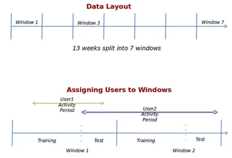
In total the applications spanned 13 weeks. This period had been divided in seven parts called windows and each users or job posting has been assigned
Figure 2.4: Overview of the time windows from which data has been taken. to only one of these windows. Job is assigned to a window with a probability proportional to the time it was public on the site in that window. Each user is assigned to a window with a probability proportional to the number of applications made by him in that window and during that window. Each window is split in two parts: train split and test split. All data are stored in relational tables contained in the following file:
• Window_dates.tsv that contains information about timing of each window.
• users.tsv that contains information about users. Each user is identified by ID called UserID.
• test_users.tsv contains a list of the Test UserIDs and windows. • user_history.tsv contains information about users’ work history. • jobs.tsv contains information about job postings.
• splitjobs.zip contains the same information of jobs.tsv but with jobs grouped in the timing windows.
• apps.tsv contains information about applications. • popular_jobs.csv is a submission file.
Figure 2.5: Users table view using Pandas
2.3.1
window_dates.tsv
This file, as the others, contains data and it is a tsv format file that means tab separated value. Each value inside the file is separated from the others by using a TAB. In this file there is a relational table that contains information about time and windowing. It is divided in 4 columns:
• Window this column contains the window ID as an integer.
• Train Start. It is a date and it represents the beginning time of the train split.
• Train End / Test Start. It is a date and it represents the end of train split and the beginning of the test split.
• Test End. It is a date and it represents the end of the test split. This table contains 7 rows, one for each window.
2.3.2
users.tsv
This file contains information about all the users in the system and these infromation are spread over 15 columns:
• UserID and WindowID. These two columns contain two integers which identify the user and the window in which user has been assigned to. • Split that contains a string that represents the split (train or test). • City, State, Country and ZipCode contain information about where
user lives. Users are from 10734 different cities, from 221 states and from 120 countries.
Figure 2.6: user_history table view using Pandas
• DegreeType, Major and Graduation Date. They contain informa-tion about the educainforma-tion level of the user. DegreeType is a value from seven: None, High School, Associate’s, Bachelor’s, Master’s, PhD, Voca-tional.
• WorkHistoryCount, TotalYearsExperience, CurrentlyEmployed, ManagedOthers, ManagedHowMany. They contain information about professional career of the users.
This table contains a lot of information about users but some of them like Major are hand-written by the users. In the whole dataset users are 389708
and this table contains NaN values.
2.3.3
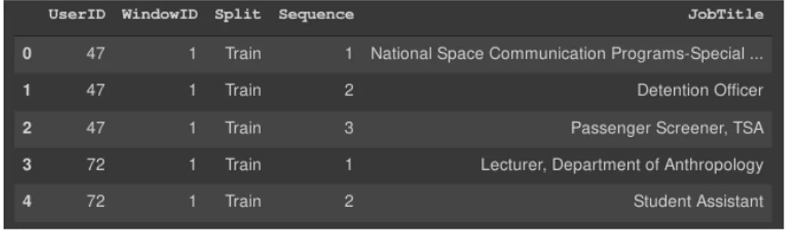
user_history.tsv
This file contains a table in which there are users’ job histories. This table has four columns:
• UserID and WindowID. These two columns contain two integers that identify the user and the window in which user has been assigned. • Split that contains a string that represents the split (train or test). • Job Title that contains the title of the job hand-written by the user. • Sequence. It is an integer number that indicates the position of the job
inside the sequence. 1 for the first, 2 for the second and so on.
This file contains one job history for each user, but in this table users are 375531 that means not all the users in the system have submitted their job histories. There are 14177 users without any indication of their past jobs.
check the description.
• City, State, Zip5 and Country contain information about where com-pany resides. Job Posting are from 11074 different cities, from 60 states and from 66 countries.
• StartDate and EndDate. These two columns are the beginning and the end of the period job posting is public.
The title, description and requirements fields are hand-written by the Company. The total number of job posting in the table is 1091923.
2.3.5
apps.tsv
This file contains a table with the application submitted by the users to a job posting in the related table. It is composed by 5 columns:
• JobID, UserID and WindowID. These three columns contain integers which identify the Job posting, the users and the window which job application has been done.
• Split that contains a string that represents the split (train or test). • ApplicationDate contains the dates when application has been done. This table contains 1603111 job applications.
2.3.6
Other files
The other files in the dataset contain the same information or information obtainable from the file described above. test_users.tsv is a table containing users for whom to predict the applications in a given window for the challenge submission. splitjobs.zip contains the same table as jobs.tsv but job posting are grouped in windows according to their visible period.
2.4
Contribution of this work
During the progresses of the project a lot of technologies have been tested but, after all of this work, two models were created. These models reached very good results opening the path to new researches in this field. Today, the most used method to approach this kind of task is to convert jobs and structured information into some vector representations using specific models or algorithms and to use another model for the prediction or the recommendation. All of this system is based on very structured data.
In this work the best results have been reached using the same model for both the duties. This model is RoBERTa3.6 model that was fine-tuned and trained for the specific task. It is capable to understand, given a job history and some user information, if the last job is part or not of the given job history with a precision of 74%. It is also capable reading a users’ job history and a job posting, to say with a precision of 92.527% if the given job posting has been submitted by the users in input.
These results underline that this kind of approach and new technologies can help to create very precise Recommendation System, even without well structured data, but they still have some limitations. For both tasks the model is the same, it is RoBERTa default model, but it has been trained on different task specific datasets.
important in order to fully understand the context of this work.
3.1
Attention Mechanism
[14] For years Recurrent Neural Networks like LSTM[15] or GRU[16] have represented the best solution to work with information modelled by sequences of data. Despite achieving better performances compared to purely statistical methods, the RNNs-based network suffers from two serious drawbacks. They are forgetful meaning old information tends to disappear after multiple steps and, second, there is no explicit word alignment. To address these problems, Attention Mechanism was introduced in neural network in particular in neural network translation machine. The basic idea of this new mechanism is to create a Context c for each data in the sequence. Each data is represented by a vector v and this context contains information about similarity with other data in the sequence in order empower latent relationship between data. In other word, using attention mechanism, model wonders on which other part of the input sequence should pay attention to fully understand a given data.
3.1.1
First implementation
To formally discuss about attention mechanism it is necessary to define V = {~vi} ∈ Rnxdv as a sequence of vectors. First of all it is needed to compute
a vector ~α called Attention Score
Figure 3.1: Graphical representation of attention during translation ei = a(~u, ~vi) (3.1) αi = ei P iei (3.2) In the first equation ~u ∈ Rd
u is the vector in the input that is going to
be matched with all the others. It is called Pattern Vector. This match is performed using a function a(~u,~v) that produces a scalar score ei that indicates
the quality of the match. After that, those scores are normalized to create the final α that can be used to compute the context vector c:
c =X
i
αi~vi (3.3)
3.1.2
Multi-Dimensional Attention
The previous kind of attention mechanism can be seem as a 1D attention because ~α is a vector containing the normalized score. Multi-Dimensional Attentionis proposed to improve the previous simple mechanism to work with more complex relationships and to capture multiple interactions between terms in different representation spaces. The idea is to map vectors to K different
3.1.3
Self Attention
Self attention is a special attention mechanism where the pattern vector u is not independent from V , like in the classic implementations, but its a part of it. In this approach V is split in many v that, one per step, become the u. Self attention was created to better model the latent relationships between the various parts of the same sequence. This kind of attention is wide used in Transformers3.4. a = sof tmax(~uK T √ dk )V (3.5)
The above equation is the typology of Self Attention adopted by Trasformers. In this kind of mechanism ~u is the part of the input sequence, Knxd is the
matrix of the keys with one row for each data in the input sequence and Vnxd
is a matrix of the values similar to K. Both are created multiplying the input sequence to two matrices: Wk for keys and Wv for the values. This procedure
is repeated for each part of the sequence.
3.1.4
Conclusion
Attention mechanism proved itself to reach better result even than Recur-rent Neural Networks. It is used with success in Natural Language Processing Tasks to create Context Word Embeddings, but also in image recognition tasks used in combination with a Convolutional Neural Network[17]. Despite its wide usage a deep formal and mathematical justification about it success is still needed and searched. It could be useful to find it in order to improve this mechanism and to apply it into different fields.
Compared to its wide usage in various NLP tasks, attempts to explore its mathematical justification still remain scarce. Recent works that explore its application in embedding pre-training have attained great success and might be a prospective area of future research - Dichao Hu[14]
3.2
Flair and Contextual String Embedding
[7] A crucial component of each Natural Language Processing Task is the word embeddings. Their quality impacts heavily on the results of the model and recent studies have underlined their importance. Find the best word embeddings is the goal for a lot researchers nowadays. The state of art methods to create them are three:
• Classical word embeddings pre-trained over very large dataset. They aim to capture latent semantic and syntactic similarities
• Character-level features[18]. They are not pre-trained but generated using task data to better represent task features.
• Contextual Word Embedding[19] that represent word in the context to address problems as polysemous.
The idea behind the Contextual string embeddings is to combine the attributes of the above embeddings in order to create best vector representations. According to the result of recent works[20] that show how natural languages can be modelled using probability distribution over characters instead words, these Contextual String Embeddings come from a Character Level Neural Model. This kind of vectors reached state of art in some NLP task as NER, PoS, . . .
3.2.1
Experiments and Results
The proposed embeddings have been compared with the other kinds in the following tasks:
• Named entity recognition using both CoNLL03 English and German. Data contains entity of four types PER for person, ORG for organization, LOC for location and MISC for miscellaneous names.
• Chunking using CoNLL2000. The task consists in dividing a text in syntactically correlated parts. It is an intermediate step toward full parsing.
• Part of Speech tagging using data from The Penn Treebank Project (https://web.archive.org/web/19970614160127/http://www.cis.upenn.edu/
tree-bank/)
Furthermore the contextual string embeddings used for testing and evalua-tions are generated using 4 different approaches.
Figure 3.2: Results obtained by using Contextual String Embeddings • Proposed + word. An extension in which they concatenate pre-trained
static word embeddings with Contextual String Embeddings.
• Proposed + char. Similar extension in which they concatenate task trained character embeddings to their Contextual String Embeddings. • Proposed + word + char where concatenation is made by using
Contextual String Embeddings, word embedding, task trained character embeddings.
• Proposed + all putting every kind of embedding together.
In each task Contextual String Embeddings help model to reach state of art. Results are shown in the figure3.2
3.2.2
Model
The selected model for the generation of these kind of Contextual String Embeddings is a bidirectional Long Short Term Memory (LSTM). It is a famous variant of Recurrent Neural Network the got recent success. Atomic input units are the characters so, at each step, the network has an internal representation of the current character given by its hidden states. The target of this model, as each character level models, is to estimate a good probability distribution
Figure 3.3: Bidirection LSTM Neural Network over characters of the input language.
P (C) =
T
Y
t=0
P (ct|c0:t−1) (3.6)
The above equation shows the target function in which C is the set of all characters in the input sentence < c0, ..., cn> and P (ct|c0:t−1 is the probability
assigned to ct to appears after c0:t−1. Training the model to generate a good
probability distribution forces it to well understand characters, relationships between them, words, sentence, semantic and syntactic rules.
3.2.3
Contextual Word Embedding Extraction
From the model described above it’s possible to extract, using its internal hidden layers, information about input characters which can be manipulated to create Word Representation Vectors. To do this it is necessary to define input sentences as a sequences of characters < c0, ..., cn >. To create the
representation vector of a word w0 in the sentence model must be used in both
direction: forward and backward. Word is composed by characters and it is a sub-sequence of the sentence: < c0, ..., cb, ..., cf, ..., cn> where cb is the first
character in the word and cf the last. Model is fed in forward direction by
giving to it all characters from c0 to cf. In this way it can get information
from the context prior to the target word. The same process is repeated but in the backward direction using characters from cn to cb. From these two
fine-tuning it can be found at the link https://github.com/zalandoresearch/flair
3.3
ELMo - Embeddings for Language Models
3.3.1
Overview
Pre-trained word representation are the key components in many NLU tasks. A good representation of the word and its characteristics leads model to achieve better results. But a representation to be considered a good one has to be capable to model:
• Complex characteristics of word usage (Syntax and Semantics) • How these uses vary across linguistic contexts (Polysemy)
ELMo wants to address both of these challenges using a Deep Contextualized Word Representation. In order to do that ELMo is based on a Bidirectional Deep Neural Network (biLM) capable to model a word according to the context into it is inserted. But differently from other models ELMo applies a function to create the embeddings using all of the internal layers of the net rather than using just to the last one (like FlairEmbeddings. See chapter 3.2). ELMo Team claims that different layers give word representations specialized on different aspects.
Using intrinsic evaluations, we show that the higher-level LSTM states capture context-dependent aspects of word meaning (e.g., they can be used with-out modification to perform well on supervised word sense disambiguation tasks) while lower-level states model aspects of syntax (e.g., they can be used to do
part-of-speech tagging) From ELMo Paper [21]
This strategy demonstrates to work extremely well in practice improving the State-of-Art in different tasks.
Figure 3.4: LSTM Layers in ELMo Model
3.3.2
Model
ELMo Model is based on different kinds of neural network working together. There are LSTM neural network and CNN. It takes in input a sequence of words from a sentence. Each of them is turned into a matrix and it is given to a Character-level Convolutional Neural Network that, applying some filters, produces a feature vector for the input word. Feature Vector is a vector representation context-independent. To put context information into the word representation, the vector is passed to a BiLSTM with N layers. All of them produce hidden states and then, those hidden state are concatenated performing a weighted sum into a unique vector. The following lines explain the above key concept in detail in order to give to the reader a deep understanding of the ELMo model.
• Character-level CNN. ELMo needs context-independent word em-beddings to be trained. Authors chose to use Character-CNN based model. They trained a 2048 channel char-ngram CNN followed by two highway layers and a linear projection down to 512 dimension. A good overview of this part is in the paper Character-Aware Neural Lan-guage Model[2]. According to this paper the input sentence is split in word [k0, k1, ..., kj] ∈ V and each word is composed by [c1, c2, ..., cl]
characters where l is the length of the word k. Characters are turned into fixed-sized vector multiplying the one-hot encoding of the character
Figure 3.5: Character-Level CNN used in a lot of models including ELMo. Picture from paper [2]
by a weight matrix Wv. In this way a word k is represented by a matrix
Cdxl where each column is the vectoring representation of each character.
After that filters Hdxw with w ∈ W (weights of filters) are applied and for
each filter a feature vector is computed. The feature vector is generated using this formula:
fk[i] = tanh(< Ck[∗, i : i + w − 1], H > +b)
From each feature vector the max value yi is extracted to create the final
representation of the word k. If H0, H1, ..., Hi are the filters used the
final vector yk for the word k will be [yk
0, y1k, ..., yik]. After this CNN there
are placed two HighWay Neural Network [3] which give to the model the possibility to choose to apply affine function followed by a non linear function (as in a classical layer) or not. To give to the network this ability a layer in the Highway Neural Network performs this function:
y = F (x, Wf) ∗ T (x, W t) + x ∗ (1 − T (x, Wt))
So the layer is controlled by the paramenters T () and it is the net itself to choose the right value into it.
y = (
x if T (x, Wt) = 0
F (x, Wf) if T (x, Wt) = 1
• ML-biLSTM Layers. ELMo uses a Multi Layers biLSTM neural net-work. A biLSTM is the combination of two LSTM Neural Networks that have learned how to extract information from input sequence in both the directions: from beginning to the end and backward. This architecture performs very well in NLP tasks and it is wide deployed. What differs in ELMo model from others is how output is compute. In ELMo y is a weight sum of all hidden states.
ELM o(k) = γ
L
X
j=0
sj ∗ hk,j
Where k is the token in input, L the number of hidden layers, h the state of a hidden layer, s a weight vector and γ a scalar used according to the task model is performing.
3.3.3
Performances of ELMo
Authors suggest to use ELMo with another Model in order to improve the system. The Idea behind is to use ELMo just to produce better Word
Figure 3.6: Highway model. Picture from paper [3]
Embeddings so, if there is another model for a specific task, ELMo can be added anyway to improve the performances. In many benchmarks for NLP Tasks ELMo has been added to the best model and it helped to get new States of the Art.
• SQuAD. Stanford Question Answering Dataset contains more than 100K crowd sourced question-answer pairs where the answer is a span in a given Wikipedia paragraph. The previous best model was a Bidirectional Attention Flow Model[22] with 81% of F-measure. After adding ELMo as embedding components the F-measure improved by 4.7%.
• Semantic Role Labeling. This task is performed on OneNotes bench-mark with more than 2.9 million words and it consists to understand which words are the subjects, the verbs and the objects. The best score is obtained using a deep biLSTM interleaved neural network [23]. Adding ELMo the F-measure jumped up by 3.2% from 81.4% to 84.6%
3.3.4
How to use
Elmo can be used trough the AllenNLP packages for python from this site https://allennlp.org/elmo. There are also free pre-trained model available Small with 13.6M parameters, Medium with 28.0M parameters, Original and Original 5.5B both with 93.6M parameters.
3.4
Transformers
A new kind of Neural Network Architecture has recently proved his power in Sequence to Sequence tasks as translation. It is called Transformer [24] and it is created to solve a specific problem. All sequence translation models are based on complex recurrent neural network as RNN, LSTM, BiLSTM, GRU . . . . They work reading just one word per step and precluding any form of parallelization within training examples. This leads to a critical performance for wide input sentences. Transformer wants to overcome this limits but without worsening performances.
3.4.1
Overview
Transformers are build without using Recurrent Neural Network in order to untied them from input sequence constrain, however the ordering of the word is a important information for Natural Language Processing. So Transformers employ a mechanism called Attention that is often used with advanced Recur-rent Neural Network. Attention helps a Neural Network to focus on interesting elements and to ignore others. Trsformers use a special kind of attention called Self-Attention, sometimes Intra-Attention and it is a mechanism that cre-ates relationships between pieces of a single input sequence. For each piece of the sequence (like words for sentence or number for numeric series) it creates a vector representation of its relationships with other pieces and this vector is called Context Vector. This kind of attention has been used successfully in a number of NLP tasks (please refer to section 3.1.
3.4.2
Model
The Transformer architecture is based on Encoder-Decoder architecture. This kind of Neural Notwork are widely employed in Sequence to Sequence tasks because their good performances. The encoder maps a input sequence of embeddings x0, x1, ...xnto an output sequence z0, z1, ...zn. These vectors become
the input of the decoder that generates a sequence of symbols y0, y1, ...ym. Model
is auto-regressive, consuming the previously generated symbols as additional input at each step. This mechanism is shown in 3.7. Transformer encoder is composed by a stack of N = 6 layers and each layer contains two sub-layers: Multi-Head Self-Attention Layerand Feed Forward Neural Network. The output of the first sub-layer is combined with his input and becomes the input of the second sub-layer oi = LayerN orm(xi+ sublayer(xi)). This
technique is called Residual Connection. The output of the entire layer is the input of the next layer in the stack. Transformer decoder, as encoder, is
Figure 3.7: Encoder-Decoder Architecture of Transformer
composed by a stack of N = 6 layers. Each layer contains three sub-layer: two Multi-Head Self Attentionlayers and a Feed Forward Neural Network. Between each sub layer there is a Residual Connection. At the end of the Decoder stack there is a Linear Layer that takes in input zi from the decoder
with size d and generates and output y with size equal to natural language vocabulary size. After this layer there is a SoftMax Layer that generates a probability distribution over the vocabulary. A visual representation of the architecture is in the figure3.8
3.4.3
Attention Mechanism in Transformer
In both encoder and decoder there are sub-layers called Multi-Head At-tention. Attention is representable as a function Attention(K, V, Q) that produces as result Z.
• Knxd It’s a matrix containing in each row a key k that represents a value.
• Vnxd It’s a matrix containing in each row a vector of values v.
where d is the size of the model. Transformer has d = 512and uses this different kinds of this mechanism in each layer this way:
• Encoder: It use Self attention. It is performed using just input sequence X. Each xi in input is multiplied by three matrices Wk, Wv, Wq randomly
initialized. Wk is used to generate K, Wv to generate V and Wq to
generate Q. Transformer, during training phase, has to modify those matrix in order to improve the model.
• Decoder: there are two layers here which perform Attention. The first takes as input the decoder output tokens it has produced until now and works like the encoder. It converts them into vectors and perform a self attention. The second layer use a Simple Attention in fact it computes K and V using the output of encoder and Q with the output from previous layer.
3.4.4
Multi-Head Attention
Transformers adds another level of complexity to attention mechanism employing Multi-Head Attention. Instead of compute a single attention function they got better result to linearly project the queries, keys, values h times. To do it transformer uses in each Attention Level h triples of Wk, Wv, Wq.
In this way h Z are computed but at the end of each Multi-Head Attention Layer all Z are concatenated and multiplied by a weight matrix to create the output vector with the right size.
Zqxd = [Zqxd0 , Z 1
qxd, ..., Z h
qxd] ∗ Whdxd
3.4.5
Feed Forward Neural Network
Each layer in both, Encoder and Decoder, has a sub-layer containing a Feed Forward Neural Network. This Neural Network consists in two layers with
Figure 3.9: Multi-Head Attention ReLu activation function. It can be represent as:
F F N (X) = max(0, Y W1+ b1)W2+ b2 (3.9)
The output of this Sub-Layer is given directly to the Attention sub-layer of the next layer.
3.4.6
Input and Output
Transformer takes in inputs embedding representations of the words in a sentence. But the problem is that transformer can’t know the position of the word in input sentence but this information can be very interesting. To fill that lack a positional information is injected in each word embedding at the bottom of the encoder and decoder stacks. It is called Positional Encoding and it is a vector with the same size of the embeddings and each cell is filled following Sine and Cosine function at different frequencies. The value is computed using this formula: P E(pos,i)= sin( pos 10000 k dmodel ), if i = 2k cos( pos 10000 k dmodel ) if i = 2k + 1 (3.10) According to this formula all even dimensions are encoded using a sine function and all odd dimensions using cosine. The positional encoding vectors,
P (x) over the entire output vocabulary. To do that, Transformer uses two layers: a Linear Layer and a Softmax Layer. The first, which is a fully connected neural network, takes in input the output Oi from last layer of the
decoder and it produces a vector with size equal to the number of words in the output vocabulary. The SoftMax layer turns this vector in the probability distribution.
3.4.7
How to use
Transformers are freely available using the package tensor2tensor. It comes from repository https://github.com/tensorflow/tensor2tensor
3.5
Bidirectional Encoder Representation from
Transformer
Bidirectional Encoder Representation from Transformer[4] or Bert is a new language representation model created by Google AI Language Team.
3.5.1
Overview
Unlike recent language representation models, BERT model is pre-trained on unlabeled text and it was forced to retrieve information from both, left or right, contexts in all layers. It can be fine-tuned adding an output layer to create state-of-art models for a wide range of tasks such as Question Answering and Language Inference.
3.5.2
BERT Performance
Bert has proven to excel in Natural languages Understand Tasks and sometimes it has overcame the current State of The Art. Next lines contains
Figure 3.10: Accuracy for GLUE Task. Picture took from Bert Paper[4] Bert results.
• General Language Understanding Evaluation : BERT Score 80,5% (7,7% Absolute improvement). GLUE [25] is a benchmark for the eval-uation of a model on Natural Language Understanding (NLU). It com-prehends different tasks as Question Answering, Sentiment Analysis and Textual Entailment. All single task results are in the picture
• Multi-Genre Natural Language Interface (MultiNLI). BERT ac-curacy 86,7. It collects 433000 sentence pairs annotated with textual entailment information. It pairs a written or spoken text with a Hypoth-esis. Task wants the model to classify the entailment between text and Hypothesis as ENTAILMENT, CONTRADICTION, NEUTRAL.
• Stanford Question Answering Dataset 1.1 (SQuAD v1.1 []): Ques-tion answering Test F-Score 93.2. Previous F-Score was 91.2 held by Humans. This dataset is a collection of 100K crowd-sourced question/an-swering pairs. Given a sentence from Wikipedia and a question, the task is to predict the answer text span in the given passage. Sometimes question could be unanswerable and model should not answer.
• Stanford Question Answering Dataset 2.0 (SQuAD v2.0 []) BERT F1-Score 83.1. Previous best score was 78.0. This new version contains 100k more data and adding questions which need more complex answers.
3.5.3
Model
BERT architecture is just the encoder piece of the Transformer architec-ture (see section 3.4). The idea is the Transformer uses encoder to generate an embedding representation zi of a word and decoder, to fulfill the task, has to
associate to that vector a probability distribution over the output dictionary. It could be worth to use the zi representation as embedding for NLP tasks.
• Tokenization. Sentence is split in tokens using WordPiece Tokens []. It is a vocabulary of 30000 tokens and after that special tokens are added to the sentence: [CLS] at the beginning of each sentence and [SEP] to separate the first sentence to the second. Once all tokens are present they are converted into their IDs from vocabulary.
• Token Embedding. IDs are scalars. Each of them is multiplied with vector of size dmodel to generate the embedding of that token. During
train phase these vectors are modified by optimizer to generate even better embedding.
• Position Embedding As in Transformer model the positional embed-ding is add to each Token Embedembed-ding. See the section 3.4 for more details.
• Segment Embedding. When BERT deals with sentence pairs [SEP] tokens help to divide the first sentences to the seconds. To improve this separation an extra vector is used. Each sentence has its vector and it is summed to each token of the sentence. The vectors of the two sentences are different and they are modified during training phase.
3.5.5
BERT Framework
The idea behind BERT is to pre-train Encoder in order to make it learn how to represent words, latent semantics and all useful information. Once it has been trained, it can be deployed to do some NLP tasks just adding a Neural Network at the end of the encoder. This Neural Network takes as input some or all outputs from the Encoder and produces a result. This proceedings is called Fine-Tuning and it is performed trough this steps:
• Pre-training: during this phase model is trained using unlabeled data and two different tasks. The data comes from BookCorpus[26] and English Wikipedia while the tasks are:
Figure 3.11: Bert Model. Picture from Bert Paper[4]
– Masked LM Masked Language Model. In this task a token from inputs is masked using MASK token and Bert must be able to retrieves it. This process forces Bert to put attention on both directions: the piece of sentence prior to the masked word and the one after. MLM works masking some percentage of the input tokens randomly and model must predict them. The outputs corresponding to the MASKs are given to a SoftMax Layer to predict, using a probability distribution, the target word. Problem is that MASK token does not appear during fine-tuning phase. To mitigate this they take 15% of the whole tokens and the 80% of them is turned into MASK tokens, 10% of them is turned in random token and the others are left unchanged. In this way Model is obliged to learn the context of each word.
– Next Sentence Prediction (NSP). In this task BERT is fed with two sentences separated by a special token SEP and, at the beginning of them, there is a another special token called CLS. BERT must learn to classify the pair A and B as IsNext if the sentence B is the actual next sentence of A, or NotNext. To do this, the representation of CLS token is given to a classifier layer that has the duty to label the pair. For this task is used a dataset of A,B sentences where in the 50% of the time B is the actual B and 50% of the time B is replaced with a random one.
• Fine-tuning: During this phase the model is trained using supervisioned training data from other downstream tasks. The parameters of the Encoder are initialized using those from pre-training phase while an
extra layer is added at the end of the pre-trained model. According to the task this extra layer could be a SoftMax, Sentiment Classifier, Entailment Classifier, . . . . This gives to BERT the power to be used in different tasks without long training sessions.
3.5.6
How to use
BERT is freely provided by google to anyone. It comes in two versions: • base : Trained using BooksCorpus (800M words) and English Wikipedia
(2.5 Billions words). It is a model with 12 layers, 768-hidden size, 12 heads (for multi-head attention), 110M Parameters
• Large. It is trained like base version, but it deploys a bigger model with: 24 layers, 1024-hidden size, 16 heads (for multi-head attention), 340M Parameters
You can download them directly from https://github.com/google-research/bert
3.6
ROBERTA
3.6.1
Overview
After the wide success of BERT a lot of studies have been conducted in order to improve it or to overcome its limitations as the computational cost for training the model or just to finetuning it. A lot of advanced models have followed and one of them, from facebook AI and University of Washington, has reached some good results. It’s called RoBeRTa that means: A Robustly Optimized BERT Pretraining Approach.
Figure 3.13: GLUE Results for ROBERTA model
We present a replication study of BERT pretraining that carefully measures the impact of many key hyperparameters and training data size. We find that BERT was significantly undertrained, and can match or exceed the performance of every model published after it. From paper[27]
The idea behind this work is that BERT is good, but it could be better with a well studied training process. This idea leads the researchers to develop this new model that has the same architecture of BERT, but a completely different training phase.
3.6.2
ROBERTA Performances
ROBERTA training process demonstrates to improve BERT results and to reach states of art for some tasks:
• General Language Understanding Evaluation[25]. For this task model was fine tuned using two approaches:Single task where model is fine-tuned before each tasks and Esambles. As it is shown in figure it surpasses BERT in all tasks and some times it reaches the state of the art.
• RACE. In this task model has to predict the right answer from four and a given textual passage that contains information about answer. It reaches a new state of art for both tasks. Results are in figure
This proves that preforming a good training sessions it is possible to reach better results.
3.6.3
Differences from BERT
The Artificial Neural Network behind is the same for BERT and ROBERTA in fact all differences lie in the training phase. For a detailed view of the model see relative section itemize
Train Data Size. The first factors that is different from BERT is the amount of data used for training. As Baevski[28] underlines in his work, the quantity of data can improve the results of the model. So ROBERTA was trained using more data than BERT for a total of 160GB of English corpora.
• Bookcorpus[26] plus Wikipedia that is the original dataset used to train BERT.(16GB)
• CC-News. It contains 63 million English news and articles. (76 GB) • OpenWebText. It contains web contents extract from URLs shared on
Reddit. (38GB)
• Stories.[29] It contains story-like text style of Winograd schemas (31GB) Dynamic Masking. BERT relies on masking technique for training. During preprocessing phase some random words were hidden under a token MASK and model has to retrieve those words. But in this way masking was static because, in each training epoch, model has to work on the same masked words. ROBERTA training used a dynamic masking to avoid to reuse the same masks. To do that dataset was duplicated 10 times so that each sequence was masked in 10 different ways.
NSP Loss removed. BERT is trained using two different losses: Mask prediction and Next Sequence Prediction that means model has to guess the masked word and, in the meanwhile, to guess if the sentence B is the next sentence of sentence A. Some studies as Lample and Conneau[30] has questioned the necessity of the NSP loss so ROBERTA was trained without that Loss Function.
BPE[31]. Byte-Pair Encoding is method to create language dictionary with a size between 10K - 100K. BERT uses a character-level BPE vocabulary of size 30K. For ROBERTA the vocabulary raise to 50K sub-word units.
All of this training differences make ROBERTA different and better than BERT. Furthermore researchers underline that training phase still needs to be well studied.
3.6.4
How to use
Authors released the model freely using directly pytorch. They released the code for pretraining and finetuning the model at https://github.com/pytorch/fairseq
3.7
Sentence BERT
After the success of BERT some researchers started to study limits and issues of this big model in order to make it better. Roberta was created to address a bad training phase but others still exists. One of them is that Bert (and Roberta) inputs are sentence pairs and that makes Bert extremely slow in similarity comparison task. Let’s imagine having a dataset of 1M strings and we want to find the most similar string in the database to a given one. In order to fulfill this task Bert has to produce a similarity score between each couple of sentences composed by the target string and the others in the dataset and then it will be possible to find the one with the higher score. Let’s imagine now that we want to find the most similar sentence for each one in the dataset. This leads us to a task with a very elevate computational cost: 1MX1M and if we didn’t have a lot of resources we would never get the result. The heart of this problem lies in Bert’s lack of creating word embeddings but just to compute and to use them internally. Some studies in this direction have been conducted but it was impossible to find solid way to extract embeddings from the hidden layer of the model. For this reason researchers have developed Sen-tence Bert[32]. It is a modification of the BERT network using siamese and triplet networks that is able to force the model to create meaningful embeddings. Researchers have started to input individual sentences into BERT and to derive fixed-size sentence embeddings. The most commonly used approach is to average the BERT output layer(known as BERT embeddings) or by using the out-put of the first token (the [CLS] token). As we will show, this common practice yields rather bad sentence embeddings, often worse than averaging GloVe embeddings - Nils Reimers and Iryna Gurevych[32]
Figure 3.16: Results of SBERT and other models in Semantic Textual Similarity (STS) benchmark
3.7.1
Sentece-Bert Results
The word embeddings extracted from this model were compared with others extrated directly from BERT or from other models. Sentence Bert has always produced better embeddings than BERT, in fact, they were tested in different Benchmarks and the vectors created by SBERT have got the higher results.
• Semantic Textual Similarity. It as dataset that contains pairs of sentences with a score from 0 to 5 that represents semantic relatedness. As it is shown in figure 3.16 SBERT has proven itself to create good embeddings while BERT, on the other hand, reached worse results even than Glove.
• Argument facet similarity[33]. It is a dataset composed by 6000 sentential argument pairs from social media divided in three controversial topics: gun control, gay marriage and death penalty. Each pair has a value from 0 to 5 where 0 means different topic and 5 the same topic. For this task SBERT worked better than Glove but not than BERT that, reading both sentence in the same time it can use the attention on them while SBERT can’t.
Figure 3.17: SBERT Architecture for compute cosine similarity
embeddings using a logistic regression classifier already trained. This benchmark is composed by more tasks:
– MR: sentiment prediction for movie Reviews
– CR: sentiment prediction of customer product reviews
– SUBJ: subjectivity prediction of sentences from movie reviews. – MPQA: phrase level opinion polarity classification from newswire. – SST Stanford sentiment treebank with binary labels.
– TREC: fine grained question-type classification from TREC. – MRPC: Microsoft Research Paraphrase Corpus from parallel news
source.
In these embedding oriented tasks SBERT has reached the state of art for 5 out of 7 of them. Results are shown in the figure 3.15
3.7.2
Model
SBERT model is based on BERT (or ROBERTA) model adding a pooling operation to the output of BERT to derive a fixed sized sentence embedding. The pooling strategy tried are three CLS using as vector the output of class

![Figure 1.4: Picture from paper Deep Neural Networks for YouTube Recommen- Recommen-dations [1]](https://thumb-eu.123doks.com/thumbv2/123dokorg/7391123.97178/17.892.246.655.211.472/figure-picture-neural-networks-youtube-recommen-recommen-dations.webp)