SCUOLA DI SCIENZE
Corso di Laurea Magistrale in Informatica
Convolutional Neural Networks for
Image Style Transfer
Relatore:
Chiar.mo Prof.
Andrea Asperti
Candidato:
Pietro Battilana
Sessione II
Anno Accademico 2017-2018
Abstract 5
Riassunto 7
1 Introduction 9
2 Background 13
2.1 Machine Learning . . . 13
2.1.1 Artificial Neural Networks . . . 15
2.1.2 Deep Learning . . . 18
2.1.2.1 Convolutional Neural Networks . . . 18
2.1.2.2 Autoencoders . . . 19
2.2 Artistic Style Transfer . . . 22
2.2.1 Neural Style Transfer . . . 22
3 Architecture 25 3.1 Style representation . . . 25 3.1.1 Covariance matrix . . . 26 3.2 Image reconstruction . . . 26 3.2.1 Upsampling . . . 27 3.2.2 Decoder training . . . 30 3.3 Features transformations . . . 31 3.3.1 Data whitening . . . 31 3.3.2 Coloring . . . 35 3
3.4 Stylization pipeline . . . 36
4 Implementation 39 4.1 Framework . . . 39
4.1.1 Dynamic Computational Graph . . . 40
4.2 Lua dependencies . . . 41 4.3 Model definition . . . 42 4.3.1 Encoder . . . 42 4.3.2 Decoder . . . 43 4.4 Argument parsing . . . 43 4.5 Logging . . . 46 4.6 Input Output . . . 46 4.6.1 Dataloader . . . 48 4.6.2 Image saving . . . 49 4.7 Functionalities . . . 49 4.8 Model behavior . . . 50 4.9 Features WCT . . . 53 5 Evaluation 55 5.1 Results . . . 55 5.1.1 Style transfer . . . 56 5.1.2 Texture synthesis . . . 58 5.2 User control . . . 58 5.2.1 Spatial control . . . 60 5.2.2 Hyperparameters . . . 60 5.3 Performances . . . 61 6 Conclusion 63 Bibliography 67
In this thesis we will use deep learning tools to tackle an interesting and com-plex problem of image processing called style transfer. Given a content image and a style image as inputs, the aim is to create a new image preserving the global structure of the content image but showing the artistic patterns of the style image. Before the renaissance of Artificial Neural Networks, early work in the field called texture synthesis, only transferred limited and repeatitive geometric patterns of textures. Due to the avaibility of large amounts of data and cheap computational resources in the last decade Convolutional Neural Networks and Graphics Processing Units have been at the core of a paradigm shift in computer vision research. In the seminal work of Neural Style Transfer, Gatys et al. consistently disentangled style and content from different images to combine them in artistic compositions of high perceptual quality. This was done using the image representation derived from Con-volutional Neural Networks trained for large-scale object recognition, which make high level image informations explicit. In this thesis, inspired by the work of Li et al., we build an efficient neural style transfer method able to transfer arbitrary styles. Existing optimisation-based methods (Gatys et al.), produce visually pleasing results but are limited because of the time consuming optimisation procedure. More recent feedforward based meth-ods, while enjoying the inference efficiency, are mainly limited by inability of generalizing to unseen styles. The key ingredients of our approach are a Convolutional Autoencoder and a pair of feature transform, Whitening and Coloring, performed in the bottleneck layer. The whitening and coloring
transforms reflect a direct matching of feature covariance of the content im-age to the given style imim-age. The algorithm allows us to produce imim-ages of high perceptual quality that combine the content of an arbitrary photograph with the appearance of arbitrary well known artworks. With the intention to understand this unconvential approach, before diving into the architectural and implementational details, we provide an introduction to basic theoretical concepts about machine learning as well as the necessary background notions on artistic style transfer.
In questa tesi verranno utilizzati strumenti di deep learning per affrontare un interessante e complesso problema di processamento delle immagini chiam-ato trasferimento di stile. Dati in input un immagine di contenuto ed un immagine di stile, lo scopo `e di creare una nuova immagine che condivida i tratti stilistici dell’immagine di stile preservando la struttura complessiva dell’immagine di contenuto. Prima della rifioritura delle reti neurali arti-ficiali, i primi lavori di ricerca nell’ambito della sintesi di texture, erano limitati nel riprodurre texture dagli schemi geometrici e ripetitivi. Grazie alla disponibilit`a di grandi quantit`a di dati e risorse computazionali a basso costo nell’ultima decade le reti neurali convoluzionali e le unit`a di processa-mento grafico (GPU) sono state al centro di un cambiaprocessa-mento di paradigma in tutti gli ambiti di ricerca legati alla visione artificiale. Il brillante la-voro di Gatys et al. che inaugur`o il campo di ricerca chiamato Neural Style Transfer, fu il primo in grado di separare la rappresentazione dello stile e del contenuto da due immagini e ricombinarlo creando una composizione ar-tistica di alt`a qualit`a. Questi risultati sono divenuti realizzabili grazie alla rappresentazione esplicita di alto livello delle immagini estratta da reti neu-rali convoluzionali allenate su larga scala per il riconoscimento di oggetti. Questa tesi, inspirata dal lavoro di Li et al., propone un nuovo ed efficiente metodo per il trasferimento di stili arbitrari. I metodi esistenti basati su ottimizazione (e.g., Gatys et al.) producono risultati visivamente piacevoli ma sono limitati dal dispendio di tempo richiesto dalla procedura iterativa di ottimizazione. Metodi pi`u recenti basati su reti neurali feedforward godono
invece di un inferenza rapida ma sono limitati nella capacit`a di generalizzare a stili arbitrari su cui la rete non `e stata allenata. Gli ingredienti principali del nostro approccio sono una rete Autoencoder convoluzionale ed un paio di trasformazioni, chiamate Whitening e Coloring applicate sulla rappresen-tazione latente. Queste trasformazioni statistiche inducono una corrispon-denza diretta tra la covarianza della rappresentazione del contenuto e quella dello stile. Questo algoritmo ci permette di produrre immagini visimente piacevoli che combinino il contenuto di una qualsiasi fotografia con lo stile di una qualsiasi opera d’arte. Per comprendere le motivazioni di questo ap-proccio non convenzionale al trasferimento di stile, prima di addentrarci nei dettagli architetturali ed implementativi, forniremo alcuni concetti teorici sul machine learning ed alcune nozioni sullo stato della ricerca sul tema del trasferimento di stile.
Introduction
Elmyr de Hory was a Hungarian-born painter and art forger, who is believed to have sold over a thousand forgeries to reputable art galleries all over the world. The forger’s skill is a testification to the human talent and intelligence required to reproduce the artistic details of a diverse set of paintings. In computer vision, much work has been invested in teaching computers to likewise capture the artistic style of a painting with the goal of conferring this style to an arbitrary photograph in a convincing manner.
Early work on this topic concetrated on visual texture synthesis using non-parametric models for “growing” textures one pixel at a time. Soon enough, it was found out (Efros et al. [5]) that one may transfer a texture to an arbitrary photograph to confer it with the stylism of a drawing. A second line of research focused on building parametric models of visual textures constrained to match the marginal spatial statistics of texture style images. In recent years these spatial image statistics extracted from intermediate feature of state-of-the-art image classifiers proved to be superior in capturing visual textures. Pairing a secondary constraint to preserve the content of an image, as measured by the higher level layers of the same image classification network, extended these ideas into the field of Artistic Style Transfer [7]. Convolutional Neural Networks [14] are the aformentioned classifiers. These
type of model organize information about an image in a hierarchical and effi-cient way using concepts like: local receptive field, shared weights and linear downsampling. Nowdays, CNN represent the state-of-the-art for almost all image processing tasks.
Optimizing an image to obey the constraints mentioned above is computa-tionally expensive and yield no learned representation for the artistic style. A line of research addressed this problem by building a secondary network, i.e. style transfer network, to explicitly learn the transformation from a photograph to a particular painting style. Although this method provide computational speed, much flexibility is lost. A single style transfer network is learned for a single painting style and a separate style transfer network must be built and trained for each new painting style. This approach avoid the critical ability to learn a shared representation across different styles. In this thesis we proposed a simple yet effective method for universal style transfer using Convolutional Neural Networks. The transfer task is formu-lated as an image reconstruction process, with the content image features being transformed at an intermediate layer with regard to the statistics of the style image features. The signal whitening and coloring transforms (WCT) are used to match the content features to those of the style directly in the deep feature space. Transformed features are reconstructed back to RGB space by a symmetrical convolutional decoder network. The proposed method enjoys learning freeness at test-time, at the cost of training a general-purpose image reconstruction decoder in advance.
Chapters Overview
Chapter 1 briefly explains the scientific context and the objectives of this thesis.
con-cepts used throughout the rest of the thesis. It also presents the differ-ents research directions in the field of Artistic Style Transfer.
Chapter 3 describes the architecture of the proposed approach in details. Particular techniques like image reconstruction, upsampling, features whitening and coloring are analysed.
Chapter 4 explains the implementational choices made during the develop-ment process. This chapter explains the program functionalities and its user interface.
Chapter 5 showcase the stylization obtained with differents hyperparame-ters configurations. In the end, some performance remarks regarding execution time are given.
Chapter 6 draws concluding remarks on the work done and presents some future work directions.
Background
This chapter is going to review some of the basic principles and architectures used in Machine Learning, giving notions useful throughout the rest of this thesis. It will also focus on the topic of style transfer reviewing the most important research efforts in the literature and how they contributed to the current state of the art.
2.1
Machine Learning
Machine Learning is a field of Artificial Intelligence suited for problems dif-ficult to address by algorithmic means. Problems of this kind are: spam or fraud detection, recognition of object in an image or of the words in a sound recording. It is essentially a form of applied statistics trying to estimate complicated functions using the knowledge extracted from input data. The concept of learning in [19] is defined as: “A computer is said to learn from experience E with respect to some class of tasks T and performance measure P, if its performance at task in T, as measured by P, improves with experience E”. Experience is formalized as a set of examples, in turn each composed of a set of features that describe the relevant properties of the example. The implementation consist of a statistical model with a fixed number of parameters, that given an example as input, produce an output
value. The perfomance of the model is evaluated by an error measure that compute the distance between the model’s output and the correct output. The model’s parameters are optimized with respect to the perfomance metric in order to obtain increasingly better results.
This process of automatic learning is useful if our learnt approximation func-tion can perform well not only on already-seen training data but especially on unseen real-world data, thus, achieving the generalisation propriety. If the input examples are independent and identically distributed (denoted i.i.d.) the inductive learning assumption guarantees us generalisation when the ex-perience data feeded to the model is sufficiently large. This computational exstensive data-driven process is feasible nowdays thanks to the hardware improvement of the last decade.
A distinction between learning algorithms concerns how the experience data, also called dataset, encodes the function to be approximated. From that per-spective, we have supervised learning, when the target function is com-pletely specified by the training data in the form of associated labels. In an unsupervised learning setting instead, the system will learn to uncover patterns and find groups in the dataset which contain no explicit descrip-tion of a target concept. Unsupervised learning involves observing several examples of a random vector of feature x and attempting to implicitly or explicitly learn the probability distribution p(x) that generated the dataset; while supervised learning involves observing several examples of a random vector of features x and an associated value or vector y, then learning to predict y from x, usually by estimating the conditioned probability p(y|x).
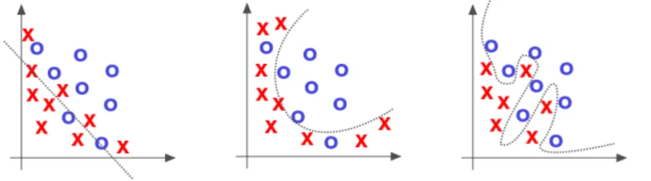
The process of learning can be seen as a search in a function space H = h | h : X −→ Y for the function h that fits better the not-known target func-tion f according to the error measure. If the model h is too complex and specialized over the peculiarities of the instances of the training set we are in a situation of overfitting; instead if the model is too simple and does not
Figure 2.1: Supervised learning (left) find the best fitting line to categorize data points vs Unsupervised learning (right) discover structural properties of the feature space as grouping (also called clusters).
allow to express the complexity of the observations (low capacity model) we are in a situation of underfitting. This is illustrated by Figure 2.2
Figure 2.2: Approximation possible outcomes: underfitting (left), desired (center), overfitting (right).
2.1.1
Artificial Neural Networks
Under the field of Machine Learning there is a family of models that take their inspiration from the way the brain is configured. The brain is composed by a huge amount (around 1011) of neurons connect together in a very big
and intricate and network. Neurons send informations to others neurons through an axon and receive informations through structures called synapses (approximately 103 synapses per neuron). Artificial Neural Networks (ANN), also just called Neural Networks, use this connectionist approach for decision
making and learning.
The basic unit of a Neural Networks is an artificial neuron. Its main job is to compute a weighted linear combination of the inputs received from other neurons. The result is then passed into a particular nonlinear function called activation function. The result of such function is the output of a neuron and gets immediately propagated to others. The idea of an artificial neuron was developed in the 1950s and 1960s by the scientist Frank Rosenblatt [21], inspired by earlier work by Warren McCulloch and Walter Pitts [18].
The first artificial neuron was called perceptron. It had binary inputs and a binary output computed by a step function that emitted 1 if the input was larger than some fixed threshold. Networks made of perceptrons were expressive enough to calculate every boolean function. The problem of the perceptron was its mathematical instability when updating the weights due to the step function shape.
Research on the field led to better perfoming activation functions. In partic-ular, the sigmoid function has a shape similar to a threshold function but has the benefit of derivability in all its real-valued domain. Derivability plays a major role in the optimization of such neural networks as we will see shortly.
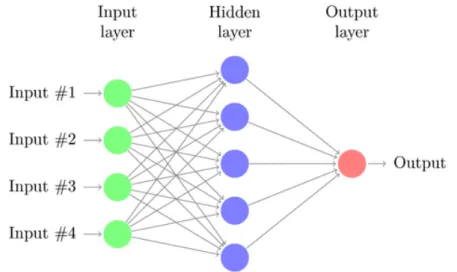
The principal kind of Artificial Neural Networks are feedforward models. The neuron’s topology of such models is a directed directed acyclic graph (i.e., no loops and backward connections). Among feedforward models, the Multi Layer Perceptron (MLP) is the most basic architecture. We can see an example of it in Figure 2.3. Neurons are grouped in layers, which are stacked one next to each other. The input values flows forward from the input layer to the output layer triggering the computation at each layer. The expressive power of ANN comes from the nonlinearity of the activation function, allowing MLP with hidden layers to approximate any nonlinear function (universal approximation theorem [9]).
Figure 2.3: Example of a feedforward neural network with 4 neurons in the input layer, 5 neurons in the hidden layer and only one neuron in the output layer. Such small ANN can be trained to perform tasks like binary classification or logistic regression.
The largest difference between linear models and ANN regards training pro-cedure and the fact that the nonlinearity of neural networks causes the loss function to be nonconvex. This means that neural networks are usually trained by using iterative gradient-based optimizer algorithms that drive the loss function to a very low value. Stochastic Gradient Descend is the most used optimization algorithm of this kind. It doesn’t have a conver-gence guarantee and it is sensible to the initial configuration of the model’s parameters.
The aformentioned optimization algorithm repeats a two phase cycle: for-ward propagation and parameters update. After evaluating the model on some input vector, the derivatives of the loss function with respect to the model’s parameters are computed at each neuron. The optimizer implement this by calling an internal procedure called back-propagation that use the chain rule of calculus to calculate derivatives efficiently. These derivatives, also called gradients, are used by the optimizer to adjust the model’s
param-eters in the attempt to find a global minimum of the loss function.
2.1.2
Deep Learning
Very simply, a neural network with more than one hidden layer is called deep. Deep models in the recent years outperformed the former state of the art in a lot of tasks. We will briefly investigate the reason of this improvement and later we will consider various deep architectures.
The curse of dimensionality is the problem that arise when dealing with high dimensional random variables that can have an exponantial number of configurations. Since the order of possible configurations is computationally intractable, a good generalisation on unseen inputs seems to be very difficult if not an impossible goal to achieve [1].
Deep learning exploits the powerful prior of compositionality allowing com-plex features to be computed in terms of simpler ones in a hierarchical or-ganization. These models are powerful and flexible approximators and are capable, for example, of understanding text or images but they need a lot more training data than “shallow” networks.
Training deep models is not an easy task for various mathematical problems like vanishing gradient, local minimums and overfitting. Dropout is a tech-nique that usually helps alleviate these problems by removing with a fixed probability some neuron connections temporarily.
2.1.2.1 Convolutional Neural Networks
In the last decade these kind of deep neural networks gained popularity and established themselves as the gold standard for AI tasks regarding com-puter vision. The key ingredients of their expressiveness and efficiency are: loose connectivity (a neuron is only influenced by a small subset of adja-cent neurons) and shared weights (every neuron act as a convolutional filter performing the same operation on different areas of its input).
If we were to process an image of size n × n with a MLP we would have to use one neuron per pixel for a total of n2 neurons and n3 parameters in the
input layer. Local connectivity drastically reduce the number of parameters improving efficiency and reducing overfitting risk. This approach works really well on images because the relevant characteristics of a photo are usually formed by pixels near to each other.
Performing a convolution, as shown in Figure 2.4, can also be seen as ap-plying a filter to an image. During training we let the network learn the right sequence of filters, adjusting weights during backpropagation phase, to perform better for the task at hand.
A convolutional filter work on all input channels combining them in one feature map. If we consider the output of all the convolutional filters inside a convolutional layer we are dealing with a feature volume that can take up a lot of memory for big input images.
It is common to periodically insert a pooling layer between successive con-volutional layers. Its goal is to progressively reduce the spatial size of the representation to reduce the amount of parameters and computation in the network. This layer operates by sliding like a convolutional filter and resize the input spatially using a simple max or average operation on a group of adjacent pixels.
CNN for image recognition tasks have a few fully connected layers at the end for making the classification based on the features extracted from the convolutional layers as we see in Figure 2.5. These nets ouput a confidence score for each category and the highest is selected as the predicted class.
2.1.2.2 Autoencoders
An autoencoder is a neural network trained to reconstruct the input data out of a learned internal representation. Internally, it is composed of an encoder function h = f (x) which produce a compact representation of the input,
Figure 2.4: Application of a convolutional kernel to an input image. Input pixels are linear combinated with the kernel’s parameter. This operation is repeated by sliding the kernel all over the input image. The size of the out-put image, also called feature map, is determined by a few hyperparameters of the convolutional layer. These hyperparameters are: the size of the ker-nel (receptive field), the number of pixels shifted when moving the kerker-nel (stride) and the artificial enlargment of the input to allow kernel application on the borders (padding).
Figure 2.5: Representation of the VGG19 architecture [22] features volume evolution. In green we have convolutional layers, in blue max pooling layers and in purple fully connected layers.
called code, and a decoder function r = g(h) that attempts the reconstruc-tion of the input to the original size.
They are trained in a self-supervised way, usually using the quadratic re-construction (input-output difference) error, to perform a form of lossy data compression that works well for data with strong correlations. AE are data-specific, which means that they will only be able to compress well data similar to what they have been trained on.
Reconstructing the input that we already have is not the main goal of the autoencoders. Since they are forced to prioritize which aspects of the in-put to encode, they often learn useful properties of the data. In fact, the low-dimensional representation learned by an autoencoder is an approxima-tion of the Principal Component Analysis (PCA). Autoencoders for different tasks (e.g. dimensionality reduction, data denoising) usually have a different architecture.
Since this thesis is about image processing, we will focus on autoencoders composed of a convolutional encoder and decoder (see Figure 2.6).
Convolu-tional Autoencoders (CAE) are state-of-art tools for unsupervised learning of convolutional filters. Features extracted by these filters can be later used to perform any task that requires a compact representation of the input, like style transfer.
Figure 2.6: Example of a fully convolutional autoencoders working on a RGB image. The convolutional decoder can use deconvolutions (also called traspose convolutions) or upsampling layers to upsample the feature maps back to the original input size.
2.2
Artistic Style Transfer
Style transfer is a topic in the field of computer vision researching the inter-play between the content and the style of images. The goal of the discipline is to produce an output image that exhibit the desired style (for example, a famous painting) while preserving the semantic content of an input image. Artistic style transfer, in the beginning, was considered to be a generalisation of texture synthesis, which study how to extract and transfer the texture from a source image to a target image. Results were usually not impressive because only low-level features were captured and transferred.
2.2.1
Neural Style Transfer
Recently, inspired by the power of Convolutional Neural Networks (CNN), Gatys et al. [7] in their seminal work, reproduced with great success the
style of famous paintings on natural images. They proposed to represent the content of a photo as the features responses from a pre-trained CNN, and to model the style of an artwork as the summary features statistics. The second-order (Gram-based) statistics they used were able to model a wide varieties of both natural and non-natural textures. These statistics represent the correlation between filters responses in differents layers of the same pre-trained CNN.
Looking at Figure 2.7 the scientific offsprings following Gatys et al. can be distinguished on how the output image is constructed.
Figure 2.7: A taxonomy of artistic style transfer techniques. For the biblio-graphic references see [10].
“Slow” methods transfers the style by iteratively optimising an image. Start-ing from an initial random noise image, these techniques perform gradient-descend optimizing a loss function often composed by a content-related com-pontent and a style-related comcom-pontent. “Faster” methods address the effi-ciency issue by putting the burden on the training stage. In fact, at testing stage the stylization is obtained quickly by a single feed-forward sweep at the
cost of training in advance a model on a large set of content images for one or more style images.
Depending on the number of artistic styles a single network can reproduce, these “Fast” methods are further subdivided into three categories: single style, multiple styles and arbitrary style. The approach we consider in this thesis belong to the latter category and it is inspired by the recent work of Li et al. [16]. It exploits a series of feature transformations in order to transfer an arbitrary style in a learning free manner.
In the proposed approach, the first few layers of a pre-trained CNN network are used as an encoder and the corresponding decoder is trained for image reconstruction. A pair of feature transforms called Whitening and Colouring Transformations (WCT) are applied on the feature maps between the en-coder and deen-coder. Denoting the content image Icand the style image Isthe
stylised output I is computed as follows: I = Dec(W CT (Enc(Ic), Enc(Is))).
The algorithm is built on the observation that the whitening transforma-tion can remove the style related informatransforma-tion from the content image while preserving the overall structure.
Therefore, receiving content activations Enc(Ic) from the encoder, whitening
transformation can filter the original style out of the content features and return a filtered representation with only content information. Then, by applying colouring transformation, the style patterns contained in Enc(Is)
are incorporated into the filtered content representation, and the stylised result I can be obtained by decoding the transformed features.
Architecture
This chapter will cover in great details the structure of the model proposed by Li et al. [16], explained briefly in the end of the previous chapther. A few sections of this chapter require some notions of statistics and linear algebra.
3.1
Style representation
The key challenge in Style Transfer is how to extract effective representation of the style and then match it to the content image. Convolutional Neu-ral Networks have proved to be very effective at capturing characteristics of images. Thus, after the seminal work of Gatys et al. almost all succes-sive approaches used the features extracted by convolutionals filters as the representation of the images.
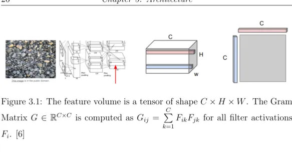
The representation encoded by the feature maps of a CNN is usually sum-marized in a statical form of features correlation called Gram Matrix. Con-sidering a feature volume as in Figure 3.1, we first reshape the tensor into a H × W grid of C-dimensional vectors. The outer products between a pair of these vectors gives a C × C matrix measuring features co-occurence of filters at these two positions. Averaging over all such matrices we get a resulting Gram Matrix of shape C × C.
Figure 3.1: The feature volume is a tensor of shape C × H × W . The Gram Matrix G ∈ RC×C is computed as G ij = C P k=1
FikFjk for all filter activations
Fi. [6]
3.1.1
Covariance matrix
The Gram matrix in [15] is empirically shown to be sensitive to features scale and poses difficulty in capturing heterogeneous style statistics. Motivated by this observation, we modify the original Gram matrix computation by subtracting F before calculating the outer products, where F is defined as the mean of all activations in the current layer of the convolutional net. This newly obtained matrix is namely the normalized covariance matrix [2], whose elements gives an estimate about how much filters activations in all feature maps share similar behaviour and variation.
3.2
Image reconstruction
Despite the recent rapid progress in Neural Style Transfer, existing methods often trade off between generalization, quality and efficiency, which means that optimization-based methods can handle arbitrary styles with pleasing visual quality but at the expense of high computational costs, while feed-forward approaches can be executed efficiently but are limited to a fixed number of styles or compromised visual quality.
The proposed approach formulate the task of style transfer as an image re-construction process, with the content features being transformed, at inter-mediate layers, with regard of style features in the midst of feed-forward
passes. This simple yet effective method enjoys style-agnostic transfer at the cost of marginally compromised visual quality and execution efficiency. The proposed architecture employ the notorious VGG19 CNN trained for the ImageNet [4] recognition task as the feature extractor. Another net is needed for inverting features back to the RGB space. This net (see Figure 3.2b) is a symmetrical VGG19 decoder responsible for the reconstruction part. The overall architecture is a general-purpose image reconstruction Convolu-tional Autoencoders. We can visualize it Figure 3.2a.
(a) The overall VGG19 convolutional autoencoder architecture used. (b) The input image reconstruc-tion task on which the autoencoder is trained.
3.2.1
Upsampling
To enlarge a input feature map produced by a CNN to a greater spatial extent the natural solution seems to be the use of traspose convolutional layers (also called deconvolutions or fractionally-strided convolutions). These layers learn
to do the reverse operation of the convolution. They take each pixel of the input image, multiply it by all the values in a n × m kernel to get a n × m weighted kernel to put in the output image. Where these kernels overlaps in the output image the values are simply summed.
The need for transposed convolutions generally arise from the desire to have a convolution’s complementary operation, in order to go from something that has the shape of the output of some convolution, to something that has the shape of its input while maintaining a connectivity pattern compatible with said convolution. In our use case, we would like to employ such operation in the decoder architecture.
Unfortunately, deconvolutions can easily have uneven overlap, in particular this happens when the kernel size (the output window size) is not divisible by the stride (the spacing between elements in the input). This leds into putting more output values in some places than others, generating bright colors and checkerboard artifacts.
These artifacts are really hard to avoid completely with traspose convolutions and doing so, often involves sacrificing some of the model’s capacity by posing restriction on the set of possible filters [20]. In addition, the presence of these artifacts doesn’t depend on the type of training done on the deconvolutional layers but it is intrinsic to the method.
Another approach to the problem, is to separate upsampling to a higher resolution from convolution to compute features. For example, you might resize the image using some linear techinque of interpolation and then do a convolutional layer. This seems to discourage high-frequency artifacts really well in a variety of training settings, for example, in Generative Adversarial Networks.
For of this motivations, the decoder designed in this thesis employ nearest neighbour upsampling layers for enlarging feature maps followed by standard convolutional layers.
Figure 3.3: The neural style transfer by Johnson et al. [11]. Stylization suffer from checkerboard artifacts (i.e. high-frequency repeating patterns) in the stylized images on the bottom.
3.2.2
Decoder training
Since successive layers of a Convolutional Neural Network encode informa-tions about an image at different levels of abstraction, it is also useful to experiment style transfer at different levels in a similar manner. For this reason we divide the VGG19 network in five blocks as denoted in Figure 3.2a. Each successive block is a sequence of convolutional and max pooling layers up to some fixed depth. These blocks are denoted “Relu X 1” where X = 1, . . . , 5 is indicating the depth of the block and “Relu” stands for Rectified Linear Unit, which is the activation function employed by VGG19.
Given the features extracted by such blocks, the authors trained accordingly five decoder blocks for image reconstruction. The loss function used for training is composed by a reconstruction loss and a feature loss. It is defined as follows:
L = kIo− Iik22+ λkφ(Io) − φ(Ii)k22 (3.1)
where Ii, Io are the input image and reconstructed output and φ is the VGG
encoder that extracts the features. In addition {λ ∈ R | 0 ≤ λ ≤ 1} is a hyperparameter to balance the two losses.
Another important aspect of the training procedure is the dataset used. In order to guarantee universal style transfer, the model, in addition to have a great approximation capacity, needs also to be able to invert features ex-tracted from a wide variety of inputs. To enable such general-purpose image reconstruction task, the COCO (Common Objects in COntext) [17] large-scale dataset was chosen for training. Created in 2014, up today it counts over 330.000 images containing complex everyday scenes with (91 different categories of) objects in their natural context.
3.3
Features transformations
This section will explain the transformations performed in the deep feature space. The input of these transformations are the feature activations of the bottleneck layer, located in the middle between the encoder and the decoder part of the convolutional autoencoder. The goal of these transformations is to combine the content with the characteristics extracted from the style in a visually pleasing way.
The type of transformations we will use are composed of two steps and are called Whitening and Colouring Transformations (WCT). These transforma-tions reflect a direct matching of feature covariance of the content image to the style image, transforming the extracted content features such that they exhibit the same statistical characteristics as the style features. They are able to achieve this goal in an almost effortless manner compared to the optimization of the Gram matrix-based cost.
3.3.1
Data whitening
Normalization is a data preprocessing technique useful in many machine learning applications. The reason comes from the fact that important pat-terns in the data often correspond to the relative relationships between the different input dimensions. Therefore, you can make the task of learning and recognizing these patterns easier by removing the constant offset and standardizing the scales. This principle gets more important when dealing with real-world data that usually have a large number of dimensions. There can now be dependencies among the dimensions, which we can think of as patterns within the data. For example, consider an image of a blue ocean (Figure 3.4) that is missing a single pixel, the value of that pixel is not independent of the nearby pixels; it is almost certainly blue.
The degree of linear dependence between the dimensions is captured by the covariance matrix cov(X) = Σ of the input data. Σ is a symmetric D × D
Figure 3.4: In order to determin the value of the missing pixel Xi
we have to consider the joint probability distribution of all the D in-put dimensions. Using the chain rule of probability this rewrites as the product of conditional probabilities p(X) = p(X1, X2, . . . , XD) =
p(X1)p(X2|X1) . . . p(XD|X1, X2, . . . , XD−1).
matrix where Σi,j contains the covariance between dimension i and dimension
j. The diagonal entries of this matrix contains the variance of each dimension. Normalization of multi-dimensional variables is called statistical whitening. Whitening is a linear transformation that transforms a vector of random variables X with a known covariance matrix Σ into a vector of new variables Z whose covariance is the identity matrix cov(Z) = I, meaning that they are uncorrelated and each have variance 1 (see Figure 3.5). The transformation is called “whitening” because it modify the input vector to resemble a white noise vector.
Formally, on input a d-dimensional vector X = (X1, . . . , XD) the result of
the whitening Z is computed as:
Z = W (x − µ) (3.2)
The input x is centered by subtracting the mean vector µ and it is multiplied by a D × D whitening matrix W . Such matrix should satisfy the conditions:
Figure 3.5: Left: the covariance matrix of the 3,072-dimensions (32x32x3) images in the notorious CIFAR10 dataset [13]. Black indicates a low value, white a high value. Dimensions are highly inter-dependent. Right: the covariance matrix after the whitening procedure. Dimensions are now com-pletely uncorrelated. cov(Z) = I ZZT = I (W (X − µ))(W (X − µ))T = I (W (X − µ))(X − µ)TWT = I W ΣWT = I W ΣWTW = W WTW = Σ−1 (3.3)
However these conditions aren’t very restrictive on W and there are actually infinetely many choices of W . This is demonstrated by the fact that taking an orthogonal matrix Q (i.e. QQT = 1), if we put W = QΣ−1/2 we get:
WTW = (QΣ−1/2)TQΣ−1/2= (Σ−1/2)TQTQΣ−1/2 =
(Σ−1/2)TIΣ−1/2= Σ−1 (3.4)
that is independent of the choice of Q. From a geometrical standpoint this phenomenon is called rotational freedom. Kessy et al. in [12] discussed the
optimality of various choices for W . Among these, Zero-phase Components Analysis (ZCA) whitening maximize the average cross-covariance between each dimension of the whitened and original data and uniquely produces a symmetric cross-covariance matrix φ = cov(Z, X). Roughly speaking, this means that it is the method preserving most of the informations in the orig-inal data minimizing the total squared distance ||X − Z||2.
ZCA whitening choice for W is W = Σ−1/2. The covariance matrix Σ by definition is assumed to be symmetric and positive semi-definite. Thus, it is possible to obtain an eingendecomposition Σ = EDET where D is the
diagonal matrix containing the eingenvalues of Σ and E is the orthogonal matrix containing its eingenvectors on the columns. The inverse square root matrix of Σ is: Σ−1/2 = ED−1/2ET where the exponentation is computed element-wise.
The overall ZCA whitening computation used in this thesis proceeds as fol-lows:
ˆ
fc= EcD−1/2c E T
cfc (3.5)
where (i) fc are the input content image features, (ii) the multiplication for
the eingenvectors matrix ET
c remove correlation between the components,
(iii) the multiplication for the scaled eingvalues D−1/2 normalize the compo-nents to unit-variance and (iv) the final multiplication for Ec “rotate-back”
data from the eingenbasis space to the features space.
The example in Figure 3.6 show a ZCA whitened image. It visually resem-ble the input image with a “washed out” effect, which remove informations related to colors and style but preserves edges and semantic content of the image. This follows from the optimality of the ZCA whitening method in maximazing the cross-covariance between the original and the whitened fea-tures.
Figure 3.6: Reconstructed whitened features. The features from VGG19 Relu 4 1 are whitened and then decoded back to original size. The whitened image maintains global content structure but style is removed (e.g., the stroke patterns of the Starry Night are gone in the whitened image).
3.3.2
Coloring
The coloring transformation shares similar spirit with the whitening trans-formation. In fact, it can be seen as an inverse of the whitening transform. It is applied to confer to the whitened features the patterns of the style image. Coloring transforms the white noise vector ˆfcinto a random vector matching
the mean and the covariance matrix of the style features fs.
The first step is always to zero-center fs by subtracting its mean vector.
Then we compute its covariance matrix Σ = fsfsT and perform an
eigende-composition yielding Σ = EsDsEsT as in the whitening procedure.
The overall coloring computation used in this thesis proceeds as follows: ˆ
fcs = EsD1/2s E T
sfˆc (3.6)
Then, we re-center ˆfcs summing the mean vector. The colored result ˆfcs will
have ˆfcsfˆcs T
= fsfsT as wanted.
To demonstrate the effectiveness of Whitening and Colouring Transforma-tions, we compare it with histogram matching, a commonly used feature ad-justament techinque. An image histogram is a chart that acts as a graphical representation of the tonal distribution in a digital image. It plots every tonal value (i.e. RGB value) present in the image on the x-axis and its frequency (i.e. number of times it appears) on the y-axis. Given two images, a refer-ence image and a target image, their histograms are calculated. Then, the
cumulative distribution functions [3] of the two histograms are computed and used to derive a mapping for every color intesity value. Then, this mapping is applied on each pixel of the reference image.
The channel-wise histogram matching [8] method determines a mapping func-tion such that the mapped fc has the same cumulative histogram as fs. As
shown in the comparison of Figure 3.7, it is clear that the HM method helps in transferring the global color of the style image but fails to capture salient visual patterns. In fact patterns are broken into pieces and local structures are misrepresented. In contrast, the proposed WCT method captures pat-terns that reflect the style image better. This can be explained by the fact that the HM method does not consider the correlations between features channels, which are exactly what the covariance matrix is designed for.
Figure 3.7: Comparison between HM and WCT coloring strategies on two differents content-style image pairs.
3.4
Stylization pipeline
So far we have developed a procedure for stylizing some reference content image to another target style style. We also know that succesive layers of a Convolutional Neural Networks represent the input at an increasingly higher level of abstraction: low-level features like edges and colors are encoded in the first layers and higher-level features like faces and objects are encoded in the last layers. This can be explained by the increasing size of receptive field and feature complexity in the network hierarchy.
organi-zation to fully capture the characteristics of style resulting in an enhanced stylization. For this purpose, it was developed an additional multi-level styl-ization pipeline. The workflow is illustrated in Figure 3.8. The content image C is input to the system only one time at the beginning. The style image S instead, is input to the system multiple times at every VGG19 block.
Figure 3.8: Multi-level stylization pipeline schematic. The result obtained by matching higher level statistics of the style is treated as the new content to continue to match lower-level information of the style.
The preffered block-ordering is descendent: the first coarse stylization I5 is
obtained from Relu 5 1 and it is regarded as the new input content image to the next stylization level that adjust lower-level features of the style. Inter-mediate results (Ix x = 5, 4, 1) are shown in Figure 3.9. These results have
the expected behaviour: higher layer features first capture the main aspects of the style and lower layer features further improve details.
(a) Content image (b) Style image
Figure 3.9: The first three images show intermediate results of the multi-level coarse-to-fine stylization pipeline. From the left respectively: I5, I4,
I1. The last image on the right is a fine-to-coarse stylization. This approach
fails because low-levels information cannot be preserved after manipulating higher-level features.
Implementation
This chapter will discuss some of the implementational choices made dur-ing the developdur-ing process of the proposed style transfer techinque. It will also give a practical explanation about the functionalities of the program and the purpose of the user arguments. Therefore, this chapter will con-tain a few source code snippets with syntax highlighting. All the source code is open-source and available at https://github.com/pietrocarbo/ deep-transfer.
4.1
Framework
The programming language of choice for the project is Python (v3.6). Launched in 1991, it had become the de-facto standard for almost all Data Science re-lated disciplines as machine learning and computer vision. It is a dynamically-typed, object-oriented, interpreted language with several functional features. Python’s dynamic nature and simple syntax make it perfect for fast pro-totyping. In fact, Data Science development process requires fast iterations with focus on data and algorithms. Moreover, Python’s open-source libraries ecosystem is mature and solid. It offers packages for almost all math and data-processing needs.
To install the needed software packages we need another tool called a package 39
manager. It is a command line application with a central repository of avail-able packages. The developer can use a package manager to install, update or remove specific packages in his system. For this project, we used the Ana-conda Python distribution that offers the largest data-science collection of packages in its repository. This distribution comes with the conda package manager, which we used to download and install packages in a project-specific virtual environment.
Maybe the most important choice about the development environment re-garded the machine learning framework to use. Even sticking only to Python, several options remain available. Keras framework it is essentially a simpler wrapper API over a more complex framework (e.g. Tensorflow). For this rea-son it doesn’t offer a lot of flexibility when implementing low-level operations in-between layers of a neural net. Since performing WCT transformations in the bottleneck layer was a requirement of the project, Keras was discarded from the options.
The choice, in the end, lied on the PyTorch framework, developed by the Facebook Artificial Intelligence Research (FAIR) group. At its core PyTorch provides tensor computations with GPU acceleration and deep neural net-works with automatic differentiation. Another important aspect is its tight integration with the Python language which make it feel more native most of the times. In fact, it shares a very similar API syntax with the notorius NumPy library for scientific computation. PyTorch is still in beta-version (v0.4.1) but has reached an important level of maturity and it’s quickly gaining momentum in the research community.
4.1.1
Dynamic Computational Graph
Another possible framework choice was Tensorflow, developed by Google Brain. It offers many of the functionalties of PyTorch; it became the stan-dard for production environments and it also offers support for mobile appli-cations. Both aformentioned frameworks operate on tensors and view models
as a directed acyclic graphs (DAG) but they differ drastically in the construc-tion of such graphs.
In TensorFlow you define graph statically before a model can run. All com-munication with outer world is performed via special objects as tf.Session and tf.Placeholder which are tensors substituted by external data at run-time. In PyTorch things are way more imperative and dynamic: you can define, change and execute nodes of a neural net as you go, without session interfaces or placeholders.
Basically, all deep learning frameworks maintain a computational graph that describe the exact order and number of operations that need to be performed. Many deep learning framwork (e.g. Tensorflow) follow a “Define and Run” philosophy, building a static data-flow graph in advance and later feed data to it. With this approach, many optimizations regarding memory alloca-tion and data parallelism are straightforward. On the other hand, newer frameworks as PyTorch follow a “Define by Run” philosophy, where the or-der and number of computations is programmatically defined. This is useful when dealing with inputs of variable size, when building Recurrent Nets used widely for Natual Language Processing tasks and, in general, whenever we want flexibility in the feedforward pass.
In PyTorch this flexibility is obtained through the Dynamic Computational Graph abstraction. In the context of this thesis’s project, this enabled to embed control-flow statements in the convolutional autoencoder’s computa-tional graph.
4.2
Lua dependencies
We already said that the proposed approach is training-free at test time. This is because the authors of the paper pretrained the five needed decoders for image reconstruction. They implemented the architecture in the Lua using
the Torch framework. Therefore, the trained models were exported in the serialization format of Torch which is t7.
PyTorch share some of the syntax and routine implementation with Torch (i.e. same C and CUDA libraries backends) and, therefore, offers a t7 deserial-ization procedure called torch.utils.serialdeserial-ization.load_lua. However, unlike the PyTorch framework, this routine is not entirely cross-platform. In fact, deserialization fails on Windows machine. Digging further it, the Torch wiki clearly states that Windows is not supported.
In order to regain platform-independence, we decided to use a third-party tool to convert t7 files in another format easier to read. This tool, on input a t7-encoded model, produces two files: a Python file containing the sequence of layer definitions (see next section) and another file with pth extension containing the model weights. The pth format is the official PyTorch binary serialization format and pth weigths can be easily loaded into an existing model with model.load_state_dict in a cross-platform way.
4.3
Model definition
In this section we will see the actual VGG19 model definition layer by layer. We will show snippets for the encoder and decoder Relu 5 1 block. Shallower blocks will not be shown because they have the same parameters but lesser layers.
4.3.1
Encoder
The encoder model in Listing 1 is an instance of torch.nn.Sequential class. The model contains layers in the order in which they are passed to the con-structor. Convolutional layers torch.nn.Conv2d have the following param-eters list (in channels, out channels, kernel size, stride=1, padding=0, . . . ).
torch.nn.ReflectionPad2d layer add a border of one pixel around the im-age using the specular pixel (i.e. the pixel at the opposite side of the imim-age). torch.nn.MaxPool2d layer look at groups of 2 × 2 pixels and retain only the maximum value.
4.3.2
Decoder
The encoder model in Listing 2 is also an instance of torch.nn.Sequential class. Padding is as in the encoder. The main difference are the torch. nn.UpsamplingNearest2d layers that act as a reverse of the MaxPooling operation and enlarge the spatial extent of the feature maps. Convolutional layer are used only to compute feature as described in section 3.2.1.
4.4
Argument parsing
The program was developed as a command-line application. The user must give the appropriate textual arguments to launch the desired task. The list of the application functionalities is discussed in the following sections. The command-line interface was written using the argparse module of the Python Standard Library. This module provides an ArgumentParser object with methods to add arguments that will be parsed from the sys.argv list. It also automatically generates help and usage messages and issues errors when users give the program invalid arguments.
In Listing 3 we can see the definition of the argument parser object with its description message. No arguments in our implementation is declared as required. At line 6 we can see the definition of a string arguments that will be stored inside parser.content, which will be the content image of the stylization. At line 10 we are defining a boolean argument with a default value of False when it is not given. At line 24 we are defining an argument which can only be a real-valued number or else the parser will trow an error. Additional checks on the arguments (i.e. existence of files and folders, floats
1 import torch.nn as nn 2
3 vgg_conv5_1 = nn.Sequential( nn.Conv2d(3,3,(1, 1)), 4 nn.ReflectionPad2d((1, 1, 1, 1)), 5 nn.Conv2d(3,64,(3, 3)), 6 nn.ReLU(), 7 nn.ReflectionPad2d((1, 1, 1, 1)), 8 nn.Conv2d(64,64,(3, 3)), 9 nn.ReLU(),
10 nn.MaxPool2d((2, 2),(2, 2),(0, 0),ceil_mode=True), 11 nn.ReflectionPad2d((1, 1, 1, 1)), 12 nn.Conv2d(64,128,(3, 3)), 13 nn.ReLU(), 14 nn.ReflectionPad2d((1, 1, 1, 1)), 15 nn.Conv2d(128,128,(3, 3)), 16 nn.ReLU(),
17 nn.MaxPool2d((2, 2),(2, 2),(0, 0),ceil_mode=True), 18 nn.ReflectionPad2d((1, 1, 1, 1)), 19 nn.Conv2d(128,256,(3, 3)), 20 nn.ReLU(), 21 nn.ReflectionPad2d((1, 1, 1, 1)), 22 nn.Conv2d(256,256,(3, 3)), 23 nn.ReLU(), 24 nn.ReflectionPad2d((1, 1, 1, 1)), 25 nn.Conv2d(256,256,(3, 3)), 26 nn.ReLU(), 27 nn.ReflectionPad2d((1, 1, 1, 1)), 28 nn.Conv2d(256,256,(3, 3)), 29 nn.ReLU(),
30 nn.MaxPool2d((2, 2),(2, 2),(0, 0),ceil_mode=True), 31 nn.ReflectionPad2d((1, 1, 1, 1)), 32 nn.Conv2d(256,512,(3, 3)), 33 nn.ReLU(), 34 nn.ReflectionPad2d((1, 1, 1, 1)), 35 nn.Conv2d(512,512,(3, 3)), 36 nn.ReLU(), 37 nn.ReflectionPad2d((1, 1, 1, 1)), 38 nn.Conv2d(512,512,(3, 3)), 39 nn.ReLU(), 40 nn.ReflectionPad2d((1, 1, 1, 1)), 41 nn.Conv2d(512,512,(3, 3)), 42 nn.ReLU(),
43 nn.MaxPool2d((2, 2),(2, 2),(0, 0),ceil_mode=True), 44 nn.ReflectionPad2d((1, 1, 1, 1)),
45 nn.Conv2d(512,512,(3, 3)),
46 nn.ReLU(),
47 )
1 import torch.nn as nn 2 3 feature_invertor_conv5_1 = nn.Sequential( 4 nn.ReflectionPad2d((1, 1, 1, 1)), 5 nn.Conv2d(512,512,(3, 3)), 6 nn.ReLU(), 7 nn.UpsamplingNearest2d(scale_factor=2), 8 nn.ReflectionPad2d((1, 1, 1, 1)), 9 nn.Conv2d(512,512,(3, 3)), 10 nn.ReLU(), 11 nn.ReflectionPad2d((1, 1, 1, 1)), 12 nn.Conv2d(512,512,(3, 3)), 13 nn.ReLU(), 14 nn.ReflectionPad2d((1, 1, 1, 1)), 15 nn.Conv2d(512,512,(3, 3)), 16 nn.ReLU(), 17 nn.ReflectionPad2d((1, 1, 1, 1)), 18 nn.Conv2d(512,256,(3, 3)), 19 nn.ReLU(), 20 nn.UpsamplingNearest2d(scale_factor=2), 21 nn.ReflectionPad2d((1, 1, 1, 1)), 22 nn.Conv2d(256,256,(3, 3)), 23 nn.ReLU(), 24 nn.ReflectionPad2d((1, 1, 1, 1)), 25 nn.Conv2d(256,256,(3, 3)), 26 nn.ReLU(), 27 nn.ReflectionPad2d((1, 1, 1, 1)), 28 nn.Conv2d(256,256,(3, 3)), 29 nn.ReLU(), 30 nn.ReflectionPad2d((1, 1, 1, 1)), 31 nn.Conv2d(256,128,(3, 3)), 32 nn.ReLU(), 33 nn.UpsamplingNearest2d(scale_factor=2), 34 nn.ReflectionPad2d((1, 1, 1, 1)), 35 nn.Conv2d(128,128,(3, 3)), 36 nn.ReLU(), 37 nn.ReflectionPad2d((1, 1, 1, 1)), 38 nn.Conv2d(128,64,(3, 3)), 39 nn.ReLU(), 40 nn.UpsamplingNearest2d(scale_factor=2), 41 nn.ReflectionPad2d((1, 1, 1, 1)), 42 nn.Conv2d(64,64,(3, 3)), 43 nn.ReLU(), 44 nn.ReflectionPad2d((1, 1, 1, 1)), 45 nn.Conv2d(64,3,(3, 3)), 46 )
in the correct interval, etc..) regarding the semantic of the application are done by the validate_args function which receives the parser object as argument.
4.5
Logging
The application execution is monitored through event logging. For this pur-pose it was used the Python Standard Library logging module. It provides a lot of flexibility and functionalities by means of:
• loggers objects expose the interface that application code directly uses. • handlers send the log records (created by a logger) to the appropriate
destinations.
• formatters are used to specify, for each handler, the layout of the log record.
In our implementation, the logger object was instantiated to output log records to two destinations: in the terminal window and in the logs.txt text file. These two handlers have been set on different severity levels: the command line handler is on a more verbose level (DEBUG) than the file handler (INFO). Following the same principle, the two handlers have a dif-ferent formatting layout. Terminal messages also contain the file and the line number from which they were generated.
4.6
Input Output
In this section we will discuss how the program read and write data, in the form of images, from and to the operative system.
1 import argparse 2
3 parser = argparse.ArgumentParser(description='Pytorch implementation ' \ 4 'of arbitrary style transfer via CNN features WCT trasform',
5 epilog='Supported image file formats are: jpg, jpeg, png') 6 parser.add_argument('--content', help='Path of the content image ' \ 7 '(or a directory containing images) to be trasformed')
8 parser.add_argument('--style', help='Path of the style image (or ' \ 9 ' a directory containing images) to use')
10 parser.add_argument('--synthesis', default=False, action='store_true', 11 help='Flag to syntesize a new texture.')
12 parser.add_argument('--stylePair', help='Path of two style images ' \ 13 '(separated by ``,'') to use in combination')
14 parser.add_argument('--mask', help='Path of the binary mask image ' \ 15 'to trasfer the style pair in the corrisponding areas')
16 parser.add_argument('--contentSize', type=int, help='Reshape ' \ 17 'content image to have the new specified maximum size') 18 parser.add_argument('--styleSize', type=int, help='Reshape ' \ 19 'style image to have the new specified maximum size')
20 parser.add_argument('--outDir', default='outputs', help='Path ' \ 21 'of the directory where stylized results will be saved') 22 parser.add_argument('--outPrefix', help='Name prefixed in the ' \ 23 'saved stylized images')
24 parser.add_argument('--alpha', type=float, default=0.2, 25 help='Hyperparameter balancing the blending between ' \ 26 'original content features and WCT-transformed features') 27 parser.add_argument('--beta', type=float, default=0.5,
28 help='Hyperparameter balancing the interpolation between ' \ 29 'the two images in the stylePair')
30 parser.add_argument('--no-cuda', default=False, action='store_true', 31 help='Flag to enables GPU (CUDA) accelerated computations')
32 parser.add_argument('--single-level', default=False, action='store_true', 33 help='Flag to switch to single level stylization')
34
35 parser.parse_args()
4.6.1
Dataloader
In most of the use cases, the user indicate as a command line argument the path of a content image and a style image. These paths can be single images or folders containing at least one image. These images should have a jpg, jpeg or png extension. Once the paths are validated, images are read into the program as PyTorch Tensors by the function load_img as in Listing 4. The open method from the PIL library is used to load the image in the standard 3-channel 8-bit RGB format at its original size. When resizing is needed, in order to keep the aspect-ratio, we need to find the image’s longer dimension. This dimension is set to the new size and the shorter dimension is scaled in order to keep the original sizes proportion intact. Lastly, the torchivision.transforms.to_tensor method converts the PIL Image with shape (H × W × C) with pixel values in the range [0, 255] to a torch.FloatTensor of shape (C × H × W ) in the range [0.0, 1.0].
1 import PIL
2 import numpy as np 3 from PIL import Image
4 import torchvision.transforms.functional as transforms 5
6 def load_img(path, new_size):
7 img = Image.open(path).convert(mode='RGB') 8 if new_size:
9 width, height = img.size
10 max_dim_ix = np.argmax(img.size) 11 if max_dim_ix == 0:
12 new_shape = (int(new_size * (height / width)), new_size) 13 img = transforms.resize(img, new_shape, PIL.Image.BICUBIC)
14 else:
15 new_shape = (new_size, int(new_size * (width / height))) 16 img = transforms.resize(img, new_shape, PIL.Image.BICUBIC) 17 return transforms.to_tensor(img)
Listing 4: Image reading function.
The object responsible for loading in images is an instance of the
abstract class torch.utils.data.Dataset, which is one of the many useful object-oriented abstractions of PyTorch. The methods to implement are: __len__ that return the total number of elements in the dataset, __getitem_ _ that return a single element of the dataset by indexing between 0 and __len__. The constructor of the ContentStylePairDataset class appends every combination of content-style paths to a list. __len__ method simply returns the lenght of this list. When requested an image, the __getitem__ method call the load_img function to load and return it.
The dataset object, in the main function of the application, is wrapped inside a Dataloader container. This provides a single or multi-process iterator over the dataset used to stylize multiple images in a single for loop.
4.6.2
Image saving
The stylized output images are saved using the torchvision.utils.save_ image function. In order to distinguish multiple outputs very easily the out-puts filenames are designed as follows:
outPrefix contentName stylized by styleName alpha alphaValue.contentExtension
The command line argument --outDir indicates a particular folder to save the ouput images in.
4.7
Functionalities
Apart from style transfer, the application offers other functionalities enabled by giving different combinations of command line arguments (see Listing 3 for the complete list). The functionalities available are:
1. style transfer. On input one content image path (--content) and one style image path (--style), the application stylize the former
ac-cording to the latter. An optional parameter --alpha (0 ≤ α ≤ 1) balance the amount of stylization and content preservation.
2. texture synthesis. On input one texture image path (--style) and the flag --synthesis, the application produce a novel texture similar to the texture given.
3. style transfer interpolation. On input a content image path (--content) and two style image paths (--stylePair) separated by a single comma, the application stylize the former according to the the characteristics of both style images. An optional parameter --beta (0 ≤ β ≤ 1) balance the transferring between the two styles.
4. texture synthesis interpolation. On input two texture image paths (--stylePair) and the flag --synthesis, the application produce a novel texture similar to both textures given.
5. spatial control. On input a content image path (--content), two style image paths (--stylePair) and a binary mask image path (--mask), the application stylize the foreground of the content image using the first style image and the background using the second style image.
4.8
Model behavior
The basic PyTorch abstraction for creating neural networks is the class torch.nn.Module. The convolutional Autoencoder, the Encoder and De-coder models we created all inherit from torch.nn.Module. The EnDe-coder and Decoder model objects as class fields of the Autoencoder. The meth-ods to implement are: __init__ that is responsible for layers definition and hyperparameter setting and forward that describes programmatically the forward pass.
The __init__ method of the Autoencoder is responsible for creating the Encoder and Decoder VGG19 blocks. The forward method of the
Autoen-coder calls the stylize function to get the result. This function passes the input to the Encoder and the Decoder blocks, that are, recalling Section 4.3, torch.nn.Sequential containers. The container, in turn, passes the input through all the layers inside it triggering the computation. To bet-ter illustrate the process, we present in Listing 5 the code of the multi-level stylization model.
The Autoencoder take as input of the constructor the command line argu-ments args. These are used to set its hyperparameters. The mask image, if present, is loaded into memory straight away. The multi-level pipeline described in Section 3.4 needs five encoder and five decoder blocks at differ-ent depths. They are instantieted and appended to the class attribute lists encoders and decoders. In the forward pass we need to perform five autoen-coder sweeps at differents depths. Thus, the forward function has a for loop iterating over the indices of the encoders list. This index is given, along with others parameters, to the stylize function responsible for encoding the images, combining with feature WCT and returning the reconstructed output.
During implementation one of the concern regarded memory saving. Our model hold in memory ten VGG19 blocks along with all their parameters. This can lead to Out of Memory (OOM) error on memory limited machines. In order to do not make the problem worse, intermediate stylization results are not kept in memory. In fact, the variable content_img at line 44 of Listing 5 is overwritten at each iteration with the latest stylization output.
OOM errors can still happen if the input images have a big resolution (i.e. usually above 1920×1080). In this case it is preferable to use the --contentSize and/or --styleSize command line arguments to resize input images instead of switching to the single-level stylization model using --single-level com-mand line argument.
1 import PIL 2 import torch
3 from PIL import Image 4 import torch.nn as nn
5 from log_utils import get_logger
6 from feature_transforms import wct, wct_mask
7 from encoder_decoder_factory import Encoder, Decoder 8 import torchvision.transforms.functional as transforms 9 log = get_logger()
10
11 class MultiLevelWCT(nn.Module): 12 def __init__(self, args):
13 super(MultiLevelWCT, self).__init__() 14 self.svd_device = torch.device('cpu') 15 self.cnn_device = args.device
16 self.alpha = args.alpha 17 self.beta = args.beta 18
19 if args.mask:
20 self.mask_mode = True
21 self.mask = Image.open(args.mask).convert('1')
22 else:
23 self.mask_mode = False
24 self.mask = None
25
26 self.e1 = Encoder(1) 27 self.e2 = Encoder(2) 28 self.e3 = Encoder(3) 29 self.e4 = Encoder(4) 30 self.e5 = Encoder(5)
31 self.encoders = [self.e5, self.e4, self.e3, self.e2, self.e1] 32 33 self.d1 = Decoder(1) 34 self.d2 = Decoder(2) 35 self.d3 = Decoder(3) 36 self.d4 = Decoder(4) 37 self.d5 = Decoder(5)
38 self.decoders = [self.d5, self.d4, self.d3, self.d2, self.d1] 39
40 def forward(self, content_img, style_img,
41 additional_style_flag=False, style_img1=None): 42 for i in range(len(self.encoders)):
43 if additional_style_flag:
44 content_img = stylize(i, content_img, style_img, 45 self.encoders, self.decoders, self.alpha,
46 self.svd_device, self.cnn_device,interpolation_beta=
47 self.beta, style1=style_img1,
48 mask_mode=self.mask_mode, mask=self.mask)
49 else:
50 content_img = stylize(i, content_img, style_img, 51 self.encoders, self.decoders, self.alpha,
52 self.svd_device, self.cnn_device) 53 return content_img
4.9
Features WCT
The source code of the Whitening and Colouring Transformations (WCT) described theoretically in Section 3.3 is given in Listing 6.
First of all, the tensor cf containing the features are converted to double-precision decimal format for the following operations. The 3D features vol-ume is reshaped to a 2D matrix using the view function. Then, each feature channel is normalized by subtracting its empirical mean before computing the covariance matrix. Since the eigendecomposition seen in 3.3 does not ex-ists for non symmetric positive-semidefinite matrices, the covariance matrix is decomposed using the Singular Value Decomposition (SVD).
The overall whitening Equation 3.5 is calculated on line 21 and the coloring Equation 3.6 have its Python counterpart on line 41. This method can be used to combine multiple feature volumes together. In fact, Listing 6 omits it for brevity but when a second style image (i.e. s1f) is given to the applica-tion, this gets also colored with the whitened features as the first style. The two colored features are blended together with a simple linear combination balanced by beta (see comment on line 47).
1 import torch 2
3 def wct(alpha, cf, sf, s1f=None, beta=None): 4 # whitening phase
5 cf = cf.double()
6 c_channels, c_width, c_height = cf.size(0), cf.size(1), cf.size(2) 7 cfv = cf.view(c_channels, -1) # new shape C × (h ∗ w)
8 c_mean = torch.mean(cfv, 1) # calculate means row-wise 9 c_mean = c_mean.unsqueeze(1).expand_as(cfv)
10 cfv -= c_mean 11 # cov(X) = Σ = XX
T
N −1
12 c_covm = torch.mm(cfv, cfv.t()).div((c_width * c_height) - 1)
13 c_u, c_e, c_v = torch.svd(c_covm, some=False) # c covm = c u ∗ c e ∗ c vT 14 k_c = c_channels
15 for i in range(c_channels): 16 if c_e[i] < 0.00001: 17 k_c = i 18 break 19 20 c_d = (c_e[0:k_c]).pow(-0.5) 21 whitened = torch.mm(torch.mm(torch.mm(c_v[:, 0:k_c], 22 torch.diag(c_d)), (c_v[:, 0:k_c].t())), cfv) 23 24 # coloring phase 25 sf = sf.double()
26 _, s_width, s_heigth = sf.size(0), sf.size(1), sf.size(2) 27 sfv = sf.view(c_channels, -1)
28 s_mean = torch.mean(sfv, 1)
29 s_mean = s_mean.unsqueeze(1).expand_as(sfv) 30 sfv -= s_mean
31
32 s_covm = torch.mm(sfv, sfv.t()).div((s_width * s_heigth) - 1) 33 s_u, s_e, s_v = torch.svd(s_covm, some=False)
34 s_k = c_channels # same as content's channels 35 for i in range(c_channels):
36 if s_e[i] < 0.00001: 37 s_k = i 38 break 39 40 s_d = (s_e[0:s_k]).pow(0.5) 41 colored = torch.mm(torch.mm(torch.mm(s_v[:, 0:s_k], 42 torch.diag(s_d)), s_v[:, 0:s_k].t()), whitened) 43
44 cs0_features = colored + s_mean.resize_as_(colored) 45 target_features = cs0_features.view_as(cf)
46 # if s1f (additional style image): cs1_features = wct(s1f) 47 # target_features = β ∗ cs0 f eatures + (1.0 − β) ∗ cs1 f eatures 48
49 ccsf = alpha * target_features + (1.0 - alpha) * cf 50 return ccsf.float().unsqueeze(0)
![Figure 2.5: Representation of the VGG19 architecture [22] features volume evolution. In green we have convolutional layers, in blue max pooling layers and in purple fully connected layers.](https://thumb-eu.123doks.com/thumbv2/123dokorg/7406675.98048/21.892.227.662.204.452/figure-representation-architecture-features-evolution-convolutional-pooling-connected.webp)

![Figure 2.7: A taxonomy of artistic style transfer techniques. For the biblio- biblio-graphic references see [10].](https://thumb-eu.123doks.com/thumbv2/123dokorg/7406675.98048/23.892.197.695.525.807/figure-taxonomy-artistic-transfer-techniques-biblio-graphic-references.webp)
![Figure 3.3: The neural style transfer by Johnson et al. [11]. Stylization suffer from checkerboard artifacts (i.e](https://thumb-eu.123doks.com/thumbv2/123dokorg/7406675.98048/29.892.217.676.360.812/figure-neural-transfer-johnson-stylization-suffer-checkerboard-artifacts.webp)
![Figure 3.5: Left: the covariance matrix of the 3,072-dimensions (32x32x3) images in the notorious CIFAR10 dataset [13]](https://thumb-eu.123doks.com/thumbv2/123dokorg/7406675.98048/33.892.164.698.136.365/figure-covariance-matrix-dimensions-images-notorious-cifar-dataset.webp)
