An introduction to stochastic volatility models

Treball final de grau

GRAU DE MATEMÀTIQUES

Facultat de Matemàtiques i Informàtica

Universitat de Barcelona

AN INTRODUCTION TO

STOCHASTIC VOLATILITY

MODELS

Autor: Matias Puig

Director:

Dr. Jose Manuel Corcuera

Realitzat a: Departament

de Matemàtiques i Informàtica

Barcelona, 29 de juny de 2017

Contents

Introduction i

1 Historical Background on Stock Price Models 3

2 Stochastic Integration 7

2.1 Martingales and Brownian motion . . . 7

2.2 Integral of mean square integrable processes . . . 9

2.3 Extension of the integral . . . 12

3 Fundamental Theorems 17 3.1 Itô’s formula . . . 17

3.2 Stochastic differential equations . . . 18

3.3 Girsanov’s theorem . . . 19

3.4 Martingale representation theorem . . . 21

4 The Black-Scholes Model 25 4.1 Risk-neutral measure . . . 26

4.2 Arbitrage and admissibility . . . 28

4.3 Completeness . . . 30

4.4 Pricing and hedging . . . 32

4.4.1 Pricing a put option . . . 33

4.4.2 Pricing a call option . . . 34

4.4.3 Hedging . . . 35

5 Stochastic Volatility 39 5.1 Empirical motivations . . . 39

5.2 A general approach for pricing . . . 39

5.3 Heston’s model . . . 42 6 Conclusions 47 7 Bibliography 49 Bibliography: Articles . . . 49 Bibliography: Books . . . 49 Bibliography: Online . . . 50 i

Introduction 1

The main goal of this work is to introduce the stochastic volatility models in mathematical finance and to develop a closed-form solution to option pricing in Heston’s stochastic volatiltiy model, following the arguments in Heston 1993.

No background in mathematical finance will be assumed, so another main goal of this work is to develop the theory of stochastic integration and to introduce the Black-Scholes market model, the benchmark model in mathe-matical finance. Standard topics in the framework of market models, such as trading strategies, completeness and replication, and the notion of arbitrage, will also be reviewed.

Chapter 1

Historical Background on Stock

Price Models

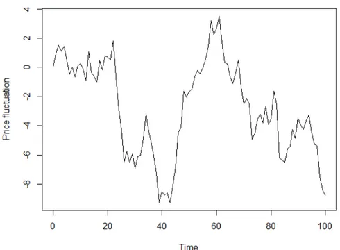
Louis Bachelier, in his thesis "Théorie de la Spéculation", made the first contri-bution of advanced mathematics to the study of finance in 1900. This thesis was well received by academics, including his supervisor Henry Poincaré, and was published in the prestigious journal Annales Scientifiques de l’École Normale Supérieure. In this pioneering work, the Brownian motion is used for the modelling of movements in stock prices. In the words of Louis Bachelier, in Bachelier 1900:

La détermination des mouvements de la Bourse se subordonne à un nombre infini de facteurs: il est dès lors impossible d’en espérer la prévision mathématique, [...] et la dynamique de la Bourse ne sera jamais une science exacte.

Mais il est possible d’étudier mathématiquement l’état statique du marché à un instant donné, c’est-à-dire d’établir la loi de proba-bilité des variations de cours qu’admet à cet instant le marché. Si le marché, en effet, ne prévoit pas les mouvements, il les consid-ère comme étant plus ou moins probables, et cette probabilité peut s’évaluer mathématiquement.

Bachelier argued that, over a short time period, fluctuations in price are inde-pendent of the current price and the past values of the price, and that these fluctuations follow a zero mean normal distribution with variance propor-tional to the time difference. He also assumed that the prices are continuous, therefore modelled as a Brownian motion (see Bachelier 2011).

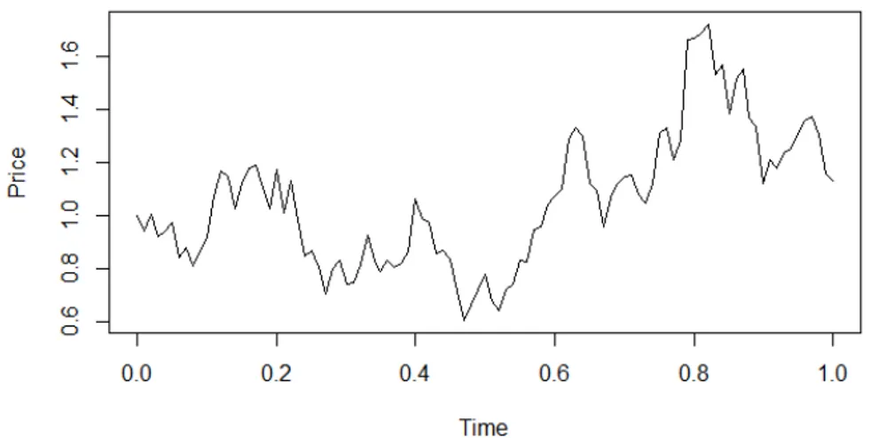
Many years later, in the famous article by Black and Scholes, Black and Sc-holes 1973, prices are modeled as a geometric Brownian motion, whose fluctua-tions have a lognormal distribution. This model is based on the assumption that the log returns of a stock price are independent and normally distributed, with variance proportional to the time difference. The log returns are defined as log(p_i) log(p_j), where p_iand p_j denote the prices at times i and j,

respec-tively, with i> j.

The returns of a stock price are defined as the increments r_i = pi pj

p_j Hence, the approxamation

Figure 1.1: Sample path of a standard Brownian motion, used by Bachelier to model fluctuations in stock prices

log(1+r) ⇡r, when r ⌧1 (1.1) Gives the approximation

p_i p_j

pj =ri ⇡log(1+ri) =log(pi/pj) =log(pi) log(pj) (1.2)

So that the lognormal distribution for the stock price increments proposed by Black and Scholes obeys to the intuitive idea that the price returns are inde-pendent and normaly distributed.

Explicitely, as stated in Black and Scholes 1973, the model proposed by Black and Scholes relies on the following assumptions of an "ideal" market:

(a) The interest rate is known and constant through time

(b) The distribution of stock prices at the end of any finite interval is lognor-mal

(c) The stock pays no dividends

(d) The variance rate of the return on the stock is constant (e) The stock price is continuous over time

Empirical observations of stock price distributions have motivated numerous extensions of the Black-Scholes model in which one or more of the previ-ous assumptions are relaxed. One of the main criticisms of the Black-Scholes model is that the normal distribution of stock price returns does not explain the significant presence of outliers in the distribution of returns (see, for ex-ample, Mandelbrot 1963). Conveniently, relaxing some of the previous as-sumptions results in distributions with a higher presence of outliers, or fatter

5

Figure 1.2: Sample path of a Geometric Brownian motion (with µ = s = 1),

used by Black and Scholes to model stock prices

tails, which better adjust to the reality of observed prices.

Examples of such extensions include models with dividend payments, stock prices with jumps (non-continuous over time), and models in which the distri-bution of returns is non-Gaussian, among others. These extensions are widely used by practitioners and are described in most text books on mathematical finance (see, for example, Musiela and Rutkowski 2006).

In this project we will concentrate on the stochastic volatility models, in which the assumption that the variance rate of the return is constant is relaxed.

Chapter 2

Stochastic Integration

Let (W,_F, P) be a probability space, and T an index set. Consider a

func-tion X(t, w) having two arguments in T and W. By fixing t, X(t,_{·) t2T} is

a family of random variables defined in W. On the other hand, by fixing w, X(·, w) _w2W can be seen as a family of ’random maps’. We will define a

stochastic process following the first point of view and show the equivalence between the two.

Definition 2.1 (Stochastic Process). Let E be a metric space with the borel s-field. A stochastic process is a family of E-valued random variables (Xt)t2T defined in a

probability space (W,F, P)

In order to define a random map as a function-valued random variable, we must specify the function space and a s-field in this space. The most natural function space to consider is the space ET of all maps from T to E. The s-field

G will be the product s-field, that is the one generated by cylinder sets of

the form p_t11(B1)\. . .\p_tn1(Bn), with B1, . . . , Bn 2 B(E) and pt being the

natural projection defined by the rule f _7! f(t).

Let (Xt)t2T be a stochastic process and define Y(w)(t) = Xt(w). Is the

map Y : (W,F, P) _{! (}ET,G) G-measurable? Indeed, for any cylinder set C = p_t11(B1)\. . .\p_tn1(Bn) 2 G, Y 1(C) = X_t11(B1)\. . .\X_tn1(Bn) 2 F.

Since_G is generated by the cylinder sets, we conclude that Y is_G-measurable. On the other hand, if Y : (W,_F, P) _{! (}ET,_G) is _G-measurable, for any

t 2 T and w 2 W define Xt(w) := Y(w)(t). Then, for any B 2 B(E),

X_t 1(B) ={w|Xt(w)2 B} = {w|Y(w)(t) 2 B} =Y 1(pt 1(B)) 2 F.

Given the equivalence between both definitions, we will consider E-valued stochastic processes on T as any of the definitions above. A sample path of X is a function x(t) = X(t, w). We say that a E-valued stochastic process on T has

paths in U ⇢ET _{if its sample paths are included in U. A stochastic process X}

is said to be continuous if its paths are included inC(T), the set of continuous

functions. The process X is continuous at t0 2 T if its sample paths x(t) are

continuous at t0 almost surely. Two stochastic processes X and Y are said to

be versions of each other if P(Xt =Yt) = 1 for all t2 T. The finite dimensional

distributions of a stochastic process X are the joint distributions of the random vectors (Xt1, . . . , Xtn), t1, . . . , tn 2 T.

2.1 Martingales and Brownian motion

We will now consider stochastic processes with the index set T = R₊, and

with values on R.

Definition 2.2 (Filtration, adapted process). A filtration(Ft)t 0is an increasing

family of s-algebras included in the s-algebra_F. A process is said to be adapted to the filtration(_Ft)t 0if for each t, Xt isFt measurable.

Given a process (Xt)t 0, we can define the natural filtration Ft =s({Xs, s 

t}), for which the process X is adapted to. Moreover, it is frequent to consider the completion of the filtration(_Ft)t 0- that is, the filtration in which all the

F-negligible sets areF0-measurable. We will refer to this filtration as the one

generated by the process X, without making explicit that it is the completion.

Definition 2.3 (Martingale). A process(Xt)t 0adapted to a filtration(Ft)t 0is a

martingale if E[_|Xt|] <• 8t 0 and E[Xt|Fs] = Xs a.s for all s <t.

The following result will be useful when defining the stochastic integral in the next section:

Theorem 2.4 (Doob inequality). If (Mt)t 0is a martingale with continuous

sam-ple paths, then:

E⇥sup tT |Mt|

2⇤

4E |MT|2

Proof. Refer to Lamberton and Lapeyre 2007 (page 58, exercise 13).

We will need some further concepts to define a Brownian motion. A stochastic process is said to have independent increments if for all 0_t1<. . . <tn, Xt1

Xt0, Xt2 Xt1, . . . , Xtn Xtn 1 are independent. It is said to have stationary

increments if for t1 <t2, Xt2 Xt1 ⇠Xt2 t1 X0.

Definition 2.5 (Brownian motion). A Brownian motion (also known as Wiener process) is a stochastic process (Wt)t 0 with continuous sample paths and

indepen-dent and stationary increments.

The following result shows further properties of the Brownian motion which are not explicit in the definition. For a proof of this result, refer to Corcuera n.d.

Proposition 2.6. Let Wt be a Brownian motion. Then Wt W0 ⇠ N(rt, s2t), for

some r2 R.

A standard Brownian motion is a Brownian motion such that W0 = 0 a.e and

Wt ⇠ N(0, t). From now on, we will usually refer to a standard Brownian

motion as a Brownian motion, without specifying that it is standard.

Proposition 2.7 (Martingale property of Brownian motion). A standard Brow-nian motion is a martingale.

Proof. Let X be a Brownian motion and s<t.

E[Xt|Fs] Xs =E[Xt Xs|Fs] =E[Xt Xs] = 0

The second equality is due to the fact that Xt Xs is independent to Fs due

to the independent increments property.

2.2 Integral of mean square integrable processes 9

Lemma 2.8. Let (Wt)t 0 be a Brownian motion under the probability P. For any

fixed M >0,

P(max

t 0 Wt(w) M) =0 P(min

t 0 Wt(w) M) = 0

Proof. This is a consequence of the distribution of the first passage time of a Brownian motion. We define the first passage time T_M to a level M ₂R as:

TM(w) =inf{t 0, Wt(w) = M}

It can be proved that the first passage time distribution has the following property (see Karatzas and Shreve 2012, p.80, equation 6.2):

P(TM <t) = 2P(Wt >M) _t !

!• 1

Since Wt is normally distributed. This proves the result, as any level M will

be reached almost surely.

2.2 Integral of mean square integrable processes

The fact that a Brownian motion is almost surely nowhere differentiable - a proof of this result can be found in Karatzas and Shreve 2012-, means that it is not possible to define the integral of a function f over a Brownian motion as

RT

0 f(s)|Ws0|ds, for any fixed T > 0. We will construct the stochastic integral

by defining it among a class of simple processes and then extend it to a larger class (as in the definition of the Lebesgue Integral). From now on, we will consider processes with an index set[0, T].

Definition 2.9 (Mean Square Integrable Process). An adapted process(Xt)t 0is

said to be mean square integrable if E(R₀TX2_tdt) < •. We will denote this class of processes as_S2.

We aim to define the integral for mean square integrable processes. By iden-tifying processes that are versions of one another and defining the natural norm _kX_k2_S2 = E(R₀TX_t2dt), it can be shown that _S2 is a Hilbert space, with

the scalar product <X, Y >=E(R₀TXtYtdt).

For constructing the integral, it is necessary to identify the so-called elemen-tary processes for which the integral can be defined trivially, and so that it can be extended to the whole_S2space.

Definition 2.10 (Simple Process). A process (Xt)tT 2 S2 is a simple process if

there exists a partition 0 = t0 < . . . < tn = T of [0, T] for which Xt = Xti for

t _{2 [}t_i, t_i+1[.

Definition 2.11. The integral of a simple process (Xt)0tT from 0 to T is defined

as:

I(X)_T =

Z _T

0 Xt dWt :=

Â

The integral process is defined as the process(I(X)t)tT, where I(X)t = I(Xs1{st}).

I(X)t = n 1

Â

Xti(Wti+1^t Wti^t)

So the integral process is pathwise continuous.

Let _{E ⇢ S}2 be the set of simple processes. Note that the integral of a simple

process is a random variable. In addition, it is in L2_{, and the integral is an}

isometry between these two spaces:

Lemma 2.12 (Isometry Property for Simple Processes). The integral defines an isometry between_E and a subspace of L2_(W,F

T, P).

Proof. Let I be the integral operator. We have to prove that:

kI(X)_k2_L2 =E h Z _T 0 Xt dW 2i =Eh Z _T 0 X 2 t dt i =_kX_k2_S2 Now, I(X)2= n 1

Â

Â

Where t0=0 and tn = T. Note that Wtj+1 Wtj is independent ofFtj and has

0 expectation.

E X_tiX_tj(Wti+1 Wti)(Wtj+1 Wtj) =E XtiXtj(Wti+1 Wti) E Wtj+1 Wtj =0

Now, applying a similar reasoning,

E[X2_ti(Wti+1 Wti)2] = E[Xt2i]E[(Wti+1 Wti)2] =E[X2ti](ti+1 ti)

Because Wti+1 Wti ⇠N(0, ti+1 ti). We obtain:

E[I(X)2] =

n 1

Â

E[X_t2_i](t_i+1 ti)

Since X is constant on every interval [ti, ti+1[, the expression above is equal

to: n 1

Â

The following result will allow us to extend the integral to the_S2 space: Lemma 2.13. The simple processes are dense inS2

The proof of this result requires several steps and will be omitted - it can be found in Karatzas and Shreve 2012 (page 134, problem 2.5). However, to give an idea on how it is accomplished, note that any continuous process(Xt)0tT

can be approximated inS2([0, T])by simple processes Xn_t defined as:

Xn_t =

T2n ₁

Â

2.2 Integral of mean square integrable processes 11

However, it is not trivial to obtain a similar result for more general adapted processes.

To extend the integral, we apply the general result that given two metric spaces X and Y and a dense subset A of X, any uniformly continuous map

f : A !Y can be extended in a unique way to X by defining ˆf(x) =lim

n f(an)

where an is any sequence in A converging to x, and this extension is well

defined and continuous. In addition, if Y is a vector space, the extension preserves the supremum norm. In our case, we can extend the integral I : E ! L2(W,FT,P) to ˆI : S2 ! L2(W,FT,P) and it remains an

isome-try.

Given a process(Xt)0tT, we define the process I(X) _tby I(X)t =R₀TXs1[0,t](s)dWs.

This process is a continuous martingale:

Lemma 2.14. [Martingale Property of the Integral] The process I(X) _t is a

mar-tingale.

Proof. Consider a first case in which X is a simple process, and let s <t. Then, we can assume tn =t and s 2 [tk, tk+1[.

Z _t 0 Xs dW = n

Â

Â

Â

Now, the first part of the last equation is an Fs measurable random variable,

so its conditional expectation toFs is the same variable.

For the second part, using the martingale property of the Brownian motion, E[Xtk(Wtk+1 Wtk)|Fs] =XtkE[Wtk+1 Wtk|Fs] = Xtk(Ws Wtk)

Finally, for j>k, and by the tower property of the conditional expectation,

E[Xtj(Wtj+1 Wtj)|Fs] = E[E[Xtj(Wtj+1 Wtj)|Ftj]|Fs] =E[Xtj(Wtj Wtj)|Fs] =0

So the last term in the equation is 0. Adding the results, we obtain: E[I(X)t|Fs] =

k 1

Â

Xti(Wti+1 Wti) +Xtk(Ws Wtk) = I(X)s

We have proven that the integral of a simple process is a martingale. To extend this result to the S2 space, it is sufficient to show that the martingale

property is preserved by limits in L2_{. This is a consequence of the fact that}

the conditional expectation is continuous in L2_{. To prove this, recall that for}

X, Y in L2_: E "_⇣ E[X|Ft] E[Y|Ft] ⌘2# =E "_⇣ E[X Y|Ft] ⌘2# EhE[(X Y)2|Ft] i =Eh(X Y)2i

Lemma 2.15 (Continuity of the integral). The process I(X) _t has almost surely

continuous sample paths.

The proof is based on the proof in Lamberton and Lapeyre 2007 (page 38, Proposition 3.4.4).

Proof. Let Xn be a sequence of simple processes converging to X inS2. Then,

by the Doob inequality,

Ehsup tT I(X n+p₎ t I(Xn)t 2 i 4E "_⇣Z T 0 X n+p s XnsdWs ⌘2# =4Eh Z _T 0 X n+p s Xns 2ds i ! n!• 0 Thus, sup tT I(X

n+p_{)t I(X}n_{)t converges to 0 in L}2_{(W,F,P), so there exists a}

subsequence f(n) such that:

sup

tT I(X

f(n+1)₎

t I(Xf(n))t _n!!_• 0, a.e

Hence, taking a subsequence if necessary, the simple (and continuous) pro-cesses I(Xf(n)) converge uniformly to I(X) almost surely, so X is almost

surely continuous.

2.3 Extension of the integral

We would like to extend the integral to the bigger space:

S = {X adapted process, P Z _T 0 |Xs| 2_{ds<• =1} } If EhR₀T_|Xs|2ds i

< •, then the set _{w,R₀T_|Xs(w)|2ds = •} must have

mea-sure zero, or otherwise the expectation of R₀T_|Xs|2ds would be infinity. So

there is an inclusionS2✓ S.

The extension can be achieved by using a technique called localization. For this, we will define the concept of a stopping time: a map t : W! T such that

{t _s_{} 2 F}s for all s 2 T . Moreover, given a process X 2 S, we say that a

sequence of stopping times tn is localising for X in S2if:

1. The sequence (t_n)n2N is increasing

2. ₈n, the stopped process X_tn = Xt1[ttn] 2 S2

3. lim

n!•tn =T, a.e.

Let X _{2 S}, and consider the increasing sequence of stopping times defined by: tn =in f n t_{2 [}0, T] Z _t 0 |Xs| 2_{ds n}o

Defined with the convention in f ∆ =T. These are indeed stopping times. To

show this, we begin by observing thatR₀t|Xs|2ds is measurable: Lemma 2.16. Given a process X 2 S,R₀tX_s2ds is _Ft-measurable.

2.3 Extension of the integral 13

Proof. Considering the integral as a Riemann integral, it can be expressed as a limit of partial sums. Then it is clear thatR₀tX2

sds is measurable, being a limit

of measurable functions almost surely. Now, for any t 2 T,

{tn >t} = {w|8st, Z _s 0 |Xu(w)| 2_{du <n} = {w|}Z t 0 |Xu(w)| 2_du<n}

Because R₀s_|Xu(w)|2du is an increasing function of s. So tn is a stopping time.

The sequence tn is localising for X in S2. Indeed, since X2 S,

a.e w 2 W, 9Nw 2 N, Z _T 0 |Xs(w)| 2_{ds <N} w So that lim

n!•tn = T, a.e. Clearly, the process Xnt = Xt1{ttn} is mean square

integrable, so we can define its integral as usual. Now, we would like to define the integral process of X as the following limit:

I(X)t = Z _t 0 XsdWs :=nlim!• Z _t 0 X n sdWs, 0 t T (2.3)

In order to prove that the integral is well defined, it is necessary to show that the limit exists, almost surely. We state this result in the following theorem:

Theorem 2.17. For any process X _{2 S}, the integral process of X as defined in 2.3 exists almost surely.

The proof is based on the one by Lamberton and Lapeyre 2007. We will need the following proposition:

Proposition 2.18. Let H 2 S2 and t be anFt-stopping time. Then,

I(H)t =

Z _T

0 1{st}HsdWs, a.s.

Proof. For any H 2 S2, we define

Z _T t HsdWs := Z _T 0 HsdWs Z _t 0 HsdWs

Let A2 Ft. The following property holds:

Z _T

0 1AHs1{s>t}dWs =1A

Z _T

t HsdWs

This is clearly true for simple processes, and the property can be extended to mean-square integrable processes by a density argument.

Now, let t = Ân

i=1ti1Ai, where all Ai are disjoint and Fti-measurable. In this

case, for each i, the process 1Ai1{s>ti}is adapted because 1Ai isFs measurable

if s>ti, and the process is zero otherwise. Hence,

Z _T 0 1{s>t}HsdWs = Z _T 0 n

Â

Â

= n

Â

Now, consider an arbitrary stopping time t and define a decreasing sequence

tn by: tn = 2n ₁

Â

Clearly, tn converges to t almost surely. Since the map t 7! R₀t HsdWs is

almost surely continuous, Rtn

0 HsdWs converges to

Rt

0 HsdWs almost surely.

By the previous discussion, we know thatRtn

0 HsdWs = RT 0 1{stn}HsdWs for all n 1. Now, E Z _T 0 1{stn}HsdWs Z _T 0 1{st}HsdWs 2! =E Z _T 0 1{t<stn}H 2 sds !

The last expression converges to 0 by the dominated convergence theorem. Consequently, Z _tn 0 HsdWs = Z _T 0 1{stn}HsdWs L2 ! n!• Z _T 0 1{st}HsdWs In particular, a subsequence ofRtn

0 HsdWsconverges almost surely to

RT

0 1{st}HsdWs.

This concludes the proof, because we also know thatRtn

0 HsdWs _n!!_•

Rt

0 HsdWs

almost surely.

Proof of the Theorem. To see that R₀tXn_{dW converges, note that because tn are}

increasing, Xn

t =1{ttn}Xtn+1. The previous proposition implies that

Z _t 0 X n sdWs = Z _t^tn 0 X n+1 s dWs

Hence, on the set_{w,R₀TXs(w)2ds <n},

I(Xn)t = I(Xm)t for all m n (2.4)

Since {w,R₀TXs(w)2ds < •} = S n2N{

w,R₀TXs(w)2ds < n} and the set has

probability 1, the sequence I(Xn)t converges almost surely.

By construction, and by 2.4, the extended integral has almost surely continu-ous sample paths. Note that the extended integral does not necessarily have the martingale property. However, we will show that it is a local martingale.

Definition 2.19. An adapted process Xt is a local martingale if there exists a

se-quence(tn)n2N of increasing stopping times such that P(lim_n tn =T) = 1 and such

that for each n, the stopped process Xtn₍t₎ :₌X_t

^tn is a martingale.

2.3 Extension of the integral 15

Proof. The proof is based on the one by Capinski, Kopp, and Traple 2012 (p.140, Proposition 4.25).

Consider again the sequence of stopping times

tn =in f n t _{2 [}0, T] Z _t 0 |Xs| 2_{ds n}o

Recall that I(X)t =_nlim

!•Mn(t), where Mn(t) := Rt 0 XsndWs is a martingale and Xn_t =Xt1{ttn}. Now, Xtk₍t_{) =} X₍t_{^tk) =} lim n Mn(t^tk) =limn Z _T 0 1[0,t^tk]X n sdWs =lim n Z _t 0 1[0,tk]1[0,tn]XsdWs = Z _t 0 1[0,tk]XsdWs = Mk(t) As for n k, tn tk.

The following result will be useful in the next sections:

Proposition 2.21. Let M be a non-negative local martingale. Then, M is a super-martingale. Moreover, if E[Mt] = M0 is constant, M is a martingale.

The proof is based on the one in Musiela and Rutkowski 2006 (p. 591, Propo-sition A.7.1). We will need the following result (see Musiela and Rutkowski 2006, p.580, Lemma A.1.2 for a proof):

Lemma 2.22 (Conditional Form of Fatou’s Lemma). Let(Xn)n2N be a sequence

of random variables in a probability space(W,F, P)and let G be a sub-s-field ofF. Suppose that there exists a random variable Z, such that Xn Z for all n, and such

that E[Z] > •. Then,

E[lim inf

n Xn|G]  lim infn E[Xn|G]

Proof. (Proposition)

Since M is a local martingale, there exists an increasing sequence of stopping times (tn)n2N such that P(lim_n tn = T) = 1 and such that for each n, the

stopped process Mtn

t is a martingale.

Let 0 _ s _ t _ T. Because M is non-negative, and by the conditional form of Fatou’s lemma,

E[Mt|Fs] = E[lim inf_n Mttn|Fs]lim inf_n E[Mttn|Fs]

=lim inf

n M

tn

s = Ms

So that M is a supermartingale.

Note that in particular, E[Mt] M0 <• for all t.

Finally, in the case of constant expectation, it is clear that if E[Mt|Fs]  Ms

Chapter 3

Fundamental Theorems

The standard results that follow are basic for the development of the mathe-matical finance theory.

Let(W,F, F= (Ft), P)be a filtered probability space, and WtanFt-Brownian

motion. We begin with the following definition:

Definition 3.1 (Itô Process). An Itô process is a process that satisfies the equation:

Xt = X0+ Z _t 0 asds+ Z _t 0 bsdWs Where: 1. X0isF0-measurable.

2. at and bt areFt-adapted and measurable processes.

3. R₀T|a_s|ds <•, a.s.

4. R₀T_|bs|2ds<•, a.s.

Equivalently, we say that the process satisfies the equation (in differential notation): dXt =atdt+btdWt

Lemma 3.2. The expression of an Itô process is unique.

Proof. Refer to Capinski, Kopp, and Traple 2012 (p. 98, Theorem 3.27).

3.1 Itô’s formula

Theorem 3.3 (Itô’s formula). Let g ₂ C1,2([0, t]_⇥R, R) and (Xt) be an Itô

pro-cess, with:

dXt =atdt+btdWt

Then Yt = g(t, Xt)is also an Itô process, and satisfies the formula:

dYt = gt+gxat+1₂gxxb2t dt+gxbtdWt (3.1)

Where all partial derivatives of g are evaluated at(t, Xt).

For a proof of Itô’s formula, refer to Capinski, Kopp, and Traple 2012 (p. 136, section 4.7). The following example will be particularly relevant:

Example 3.4. LetSt be an Itô process such that dSt =µStdt+sStdWt, and let

g(t, x) = log(x). Then, if Yt = g(t, St),

dYt = (µ 1₂s2)dt+sdWt

Or, equivalently:

St =exp (µ 1₂s2)t+sWt

We will also require a two-dimensional version of Itô’s formula, adapted from Musiela and Rutkowski 2006.

Theorem 3.5 (Itô’s formula, two dimensions). Let (W_t1), (W_t2) be Brownian

motions, g2 C1,2([0, t]⇥R2, R) and(Xt), (Yt) be Itô processes, with:

dXt =atdt+btdWt1

dYt =atdt+btdWt2

Then Zt = g(t, Xt, Yt) is also an Itô process, and satisfies the formula:

dZt = gt +gxat +gyat+1₂gxxb2t +1₂gyyb2t +gxybtbt dt (3.2)

+gxbtdWt1+gybtdWt2

Where all partial derivatives of g are evaluated at(t, Xt, Yt).

3.2 Stochastic differential equations

In the next chapter we will frequently consider stochastic differential equa-tions of the form:

dXt = a(t, Xt)dt+b(t, Xt)dWt (3.3)

X0= x0

In this situation, it is important to know if a solution to the equation exists, and in that case, if it is unique. The following theorem, adapted from Capin-ski, Kopp, and Traple 2012 (p.160, Theorem 5.8), provides sufficient conditions for this to happen.

Theorem 3.6. [Existence and uniqueness of stochastic differential equations] Con-sider the stochastic differential equation 3.3, and assume that the coefficient functions a(t, x), b(t, x) are Lipschitz with respect to x and uniformly continuous with respect

to t. Moreover, assume that they have linear growth. This means that there exists a constant C>0 such that:

|a(t, x)_{| + |}b(t, x)_{| }C(1+_|x_|), ₈x ₂R, t_{2 [}0, T] (3.4)

Then, 3.3 has a unique solution with continuous paths and that is mean square inte-grable.

3.3 Girsanov’s theorem 19

The natural extension of this result to multiple dimensions is also valid. That is, consider a multi-dimensional version of 3.3,

dXt =a(t, Xt)dt+b(t, Xt)dWt (3.5)

X0 =x0

Where (Xt) is a d-dimensional stochastic process (understood as d

compo-nents of one dimensional stochastic processes) and Wt is a d-dimensional

Brownian motion (understood as d components of one dimensional Brow-nian motions), and x0 2 Rd. Then, if the component functions a(t, x), b(t, x)

are Lipschitz with respect to x and uniformly continuous with respect to t, a unique regular solution to the stochastic differential equation exists (see Musiela and Rutkowski 2006, p.639, Theorem A.3.1).

An important property that we would like the solutions of stochastic differ-ential equations of the form 3.3 to satisfy is the Markov property.

Definition 3.7 (Markov Property). A stochastic process (Xt) in a filtered

probabil-ity space (W,_F, F, P) satisfies the Markov property if, for any bounded measurable

function f : R !Rand any s _t,

E[f(Xt)|Fs] =E[f(Xt)|FXs] (3.6)

Where (FXt)is the filtration generated by(Xt).

In our case, (_Ft) is the filtration generated by the Brownian motion (Wt).

The following result guarantees that under certain conditions on the coeffi-cient functions, this property is satisfied by solutions of stochastic differential equations. It has been adapted from Capinski, Kopp, and Traple 2012 (p.174, Theorem 5.14).

Theorem 3.8. [Markov Property] Consider a stochastic differential equation of the form 3.3, with coefficients a(t, x)and b(t, x)that are Lipshitz continuous with respect

to x, uniformly continuous with respect to t, and satisfy the linear growth condition 3.4. Then, the solution Xt has the Markov property 3.6. That is,

E[f(Xt)|FWs] = E[f(Xt)|FXs]

Proof. Refer to Capinski, Kopp, and Traple 2012 (p.174, Theorem 5.14).

3.3 Girsanov’s theorem

Theorem 3.9 (Girsanov, simple version). Let (Wt) be a standard Brownian

Mo-tion and g 2 R. Then, ˜W_t := Wt +gt is a standard Brownian motion under the

probability ˜P defined by: d ˜P

dP =exp gWT 1 2g2T

Proof. The proof has been adapted from Capinski and Kopp 2012.

It is clear that ˜W has continuous sample paths. We will prove directly that ˜

probability ˜P(A) where A = \n_i=1Ai and Ai = {W˜ti W˜ti 1  ai}, for any

given partition t0, . . . , tn ofT, and every a1, . . . , an 2 R. By definition,

˜P(A) = E_˜P⇥1_A⇤ =EP

h

exp gWT 1₂g2T 1A

i

Now, W_T can be expressed as Ân_i=1Wti Wti 1. Similarly, T =Âni=1(ti ti 1)

and 1A = n ’ i=11Ai. We obtain: ˜P(A) =E_P " _n

’

The increments Wti Wti 1 are independent, and the indicators sets Aican be

expressed as:

Ai ={Wti Wti 1+g(ti ti 1) ai}

So, because of the independence property, ˜P(A) = n

’

’

Now, because the increments Wti Wti 1 are distributed as N(0, ti ti 1),

P(A_i) = EP h exp g(Wti Wti 1) 1 2g2(ti ti 1) 1Ai i = Z { x+g(ti ti 1)ai} exp gx 1 2g2(ti ti 1) 1 p 2p(t_i t_{i 1})exp x2 2(ti ti 1) dx = Z { x+g(ti ti 1)ai} 1 p 2p(t_i t_{i 1})exp ⇣ _{x g(ti ti 1)} 2 2(ti ti 1) ⌘ dx = Z {zai} 1 p 2p(ti ti 1)exp ⇣ _z2 2(t_i t_{i 1}) ⌘ dz (3.8) Equation 3.8 proves that ˜Wti W˜ti 1 are distributed as N(0, ti ti 1), and

equation 3.7 proves that they are independent.

A generalized version of Girsanov’s theorem will be required in the Stochastic Volatility chapter. The theorem has been adapted from Musiela and Rutkowski 2006 (p.648, Theorem A.15.1).

Theorem 3.10 (Girsanov’s theorem, a generalized version). Let (Wt) be a

d-dimensional Brownian motion in the filtered probability space(W,F, F, P), and g be

an Rd_{-valued F-adapted stochastic process, such that:} E " exp⇣ Z T 0 gsdWs 1 2 Z _T 0 g 2 sds ⌘# =1 (3.9)

Define ˜Wt :=Wt+R₀tgsds, and define the probability ˜P by:

d ˜P dP =exp ⇣ Z _T 0 gsdWs 1 2 Z _T 0 g 2 sds ⌘ (3.10) Then,(W˜t)is a Brownian motion under the probability ˜P.

3.4 Martingale representation theorem 21

3.4 Martingale representation theorem

In this section, we will prove the martingale representation theorem. These re-sults have been adapted from Corcuera n.d., whose notations and arguments will be followed closely. We will need some preliminary results.

Theorem 3.11 (Martingale Lp_{-convergence). Let (Mn)}

n2N be a martingale in a

filtered probability space (W,F, F= (Fn), P). Assume that, for some p >1, Mn 2

Lp _=Lp_{(W,F, P) 8n2 N, and sup} n2N

kMnk_Lp <•. Then, for some M_• 2 Lp,

Mn L

p !

n!• M•

Proof. Refer to Kallenberg 2006 (p.109, Corollary 6.22).

Lemma 3.12. Let(Gn) be a filtration in a probability space (W,F, P) and let X 2

L2 =L2(W,_F, P). Then, E[X_|Gn] L 2 ! n!• E[X|G•] Where _G• =s(Gn, n2 N).

Proof. Define Xn := E[X|Gn]. Clearly, Xn is a martingale with respect to the

filtration (_Gn), and by the properties of the conditional expectation,

sup n2Nk Xnk_L2  kXk_L2 <• By theorem 3.11, Xn L 2 ! n!• Y

For some Y ₂ L2_{. It remains to show that Y = E[X|G}

•] =: X•. By the

continuity of the conditional expectation in L2 _{(this was proved in 2.14),} E[Y|Gn] = E[_mlim

!•Xm|Gn] =mlim!•E[Xm|Gn] = Xn

By the tower property of the conditional expectation, we also have that

E[X•|Gn] =EhE[X_|G•] Gn

i

=Xn

So that, for all n ₂ N,

E[Y|Gn] =E[X•|Gn]

Hence, for every G2 [n2NGn,

E[Y1_G] =E[X•1G] (3.11)

Define the collection

C = {G2 G• |E[Y1G] =E[X•1G]} (3.12)

Clearly, by 3.11,

[n2NGn ⇢ C ⇢ G• (3.13)

Now, if we prove thatC is a s-algebra, we will have, by equation 3.13 and the fact that_[nGn generatesG•, thatC = G•.

Condition (1) is clear since X_{2 [n2}NGn ⇢ C. For condition (2), if B⇢ A2 C,

E[Y1_A\B] =E[Y1A] E[Y1B] = E[X•1A] E[Y1B] =E[X•1A\B]

So that A\B 2 C. For condition (3) note that, if (An)n2N is a sequence in C,

by the dominated convergence theorem,

E[Y1_[nAn] =E[lim_n Y1[_m=1n Am] =lim_n E[Y1[n_m=1Am] =lim n E[X•1[nm=1Am] =E[X•1[nAn] Hence,[nAn 2 C, and C = G•. Now, Bn :={X• Y > _n1} 2 G•, so E[X•1Bn] =E[Y1Bn]

This implies that P(Bn) =08n 2N, so that P(_[nBn) =0. Hence X• Y a.s,

and a similar argument shows that X• Y a.s.

Lemma 3.13.Let(Wt)be a Brownian motion in the filtered probability space(W,F, F, P),

where F is generated by(Wt). Consider the setJ of stepwise functions f :[0, T] ! Rof the form: f = n

Â

With l_i 2 R and 0=t0<. . . <tn =T. For each f 2 J, define

E_Tf =expn Z _T 0 f(s)dWs 1 2 Z _T 0 f 2_(s)dso

Let Y 2 L2(FT, P), and assume that Y is orthogonal to E_Tf for all f 2 J. Then,

Y =0.

Proof. Let f 2 J and Y 2 L2(_FT, P)orthogonal toE_Tf. DefineGn :=s(Wt0, . . . , Wtn).

By assumption, E expn n

Â

Taking the conditional byGn we obtain: E expn n

Â

Let X : W !Rn be defined by:

X = (Wt1, Wt2 Wt1, . . . , Wtn Wtn 1) Decomposing Y as Y =Y+ Y , we get: E expn n

Â

Â

3.4 Martingale representation theorem 23

Applying the pushforward measure theorem to 3.14, and because of the fact that E[Y|Gn] =EhY _W1 =a1, . . . , Wn Wn 1=an i a1=W1,...,an=Wn Wn 1: Z Rnexp n n

Â

Â

Note that 3.15 and 3.16 are, respectively, the Laplace transforms of E[Y+|Gn](x1, . . . , xn)

and E[Y |Gn](x1, . . . , xn)with respect to the measure PX. We admit the result

on the uniqueness of the Laplace transform, which in this case implies that:

E[Y+|Gn](x1, . . . , xn) =E[Y |Gn](x1, . . . , xn), PX a.s (3.17)

So that E[Y+|Gn](x1, . . . , xn) =E[Y |Gn](x1, . . . , xn) for all(x1, . . . , xn) 2Rn\

A for some set A ⇢ Rn with PX(A) = 0. This means that E[Y+|Gn](w) = E[Y+|Gn](w), 8w 2 X 1(A). Finally,

E[Y+|Gn] =E[Y+|Gn] Pa.s. (3.18)

Since this is true for any Gn as defined above, by 3.12 we have that E[Y±|Gn] _n!!_• E[Y±|s(Gn; n2 N)] =Y±

Hence, Y =0.

Proposition 3.14. Let(W,_F, F = (_Ft), P)be a filtered probability space withF =

FT, let(Wt) be a Brownian motion and let F 2 L2(W,FT, P). Then, there exists an

adapted, mean square integrable process(Yt)such that

F =E[F] +

Z _T

0 YtdWt

Proof. Consider the Hilbert spaceHof centered random variables in L2_(W,F T, P),

and its subspace _I consisting of the random variables of the form R₀TYtdWt,

for some adapted, mean square integrable process(Yt). Note that proving the

proposition is equivalent to proving thatI = H.

If, on the contrary, I ( H, then there would exist a centered, non-trivial ran-dom variable Z 2 Horthogonal to I. We will prove that this is not possible. Indeed, suppose that such Z exists. Take Yt := E_tf, with E_tf as defined in

Lemma 3.13. Then, EhZ_· Z _T 0 E f t dWt i =0 And also EhZ_· 1+ Z _T 0 E f t dWt i =0 (3.19)

Now, a similar argument as the one in 3.4 shows thatE_tf is the solution to the following stochastic differential equation:

In particular, E_Tf =1+ Z _T 0 f(t)E f t dWt (3.20)

From 3.19 and 3.20 we conclude:

E[ZE_Tf] = 0 (3.21)

Since this is true for any f defined as in 3.13, by 3.13 we conclude that Z =

0.

Theorem 3.15 (Martingale Representation Theorem). Let(Mt) be a square

inte-grable martingale with respect to the filtration (Ft), and (Wt) a Brownian motion.

Then, there exists an adapted, mean square integrable process (Xt) such that, in

differential notation:

dMt = XtdWt, a.s

Proof. Applying the previous proposition applied to M_T, we obtain the exis-tence of a mean square integrable process(Yt) such that:

MT =E[MT] +

Z _T

0 YtdWt = M0+

Z _T

0 YtdWt

Since(Mt) is a martingale, for any t2 [0, T]we have:

Mt =E[MT|Ft] =E h M0+ Z _T 0 YtdWt Ft i =M0+ Z _t 0 YtdWt

Chapter 4

The Black-Scholes Model

The Black-Scholes model consists of two stocks S and b, in a time frame[0, T],

where b is a bank account such that b(t) = ert, and the risky stock S satisfies

the differential equation:

dSt =µStdt+sStdWt (4.1)

Where Wt is a Brownian motion in the filtered probability space(W,F, F, P),

and P represents the so-called empirical or physical probability. The dis-counted stock price is defined as S⇤

t =bt 1St.

Define F = (_Ft) to be the filtration generated by the Brownian motion (Wt).

We assume that F0 = {∆, W} and FT = F. The coefficients of the stochastic

differential equation 4.1, according to the notations in 3.3, are

a(t, x) =µx (4.2)

b(t, x) = sx

These functions clearly satisfy the regularity conditions in 3.6, so there exists a unique mean-square integrable solution St with continuous sample paths.

By theorem 3.8, this solution also satisfies the Markov property.

An explicit solution for this stochastic differential equation was found in 3.4: St =S0exp{ (µ 1₂s2)t+sWt} (4.3)

The following are some implicit assumptions of this model, as argued in Cor-cuera n.d.:

• it has continuous trajectories • its returns St Su

Su are independent of s(Ss, 0 su). Indeed,

St Su Su = St Su 1=exp{ (µ 1 2s2)(t u) +s(Wt Wu)} 1 Which is independent of s(Ss, 0 su).

• its returns are stationary:

St Su

Su ⇠

St u S0

S0

A trading strategy or strategy is a random vector f= (f1, f2)with values in R2,

adapted to the filtration (_Ft)0tT. The value of the strategy is the process

Vf(t) :=ft· (b(t), St).

A strategy is self-financing if:

dVf(t) =f1tdb(t) +f2tdSt (4.4)

This is a natural extension of the discrete time expression DnVf = f1nDnb+

f_n2DnS. The discounted value process is defined as Vf⇤(t) = ft· (1, S⇤t), where

S⇤

t =St/b(t) is the discounted stock price.

For 4.4 to make sense, we need to require that: 1. R₀T_|f1_t|dt <•, a.s

2. R₀T(f2_t)2dt<•, a.s

We will denote be the set of self-financing strategies as F. We will discuss further restrictions on the set of strategies considered in the model later on. The following characterization of self-financed strategies will be useful:

Lemma 4.1. Let f be a strategy satisfying integrability conditions (1) and (2). Then,

f₂ F iff

d ˜Vt(f) = ft2d ˜St

Proof. The proof has been adapted from Lamberton and Lapeyre 2007 (p. 65, Proposition 4.1.2).

Suppose that f is self-financing. The Itô formula gives d ˜Vf(t) = r ˜Vf(t)dt+e rtdVf(t)

Imposing the self-financing condition, we obtain:

d ˜Vf(t) = re rt(f1tert+f2tSt)dt+e rt(f1tdb(t) +f2tdSt)

=f2_t( re rtStdt+e rtdSt) =f2td ˜St

The converse can be proved similarly.

4.1 Risk-neutral measure

A risk-neutral measure is a measure ˜P equivalent to P such that the discounted stock price is a martingale under ˜P. The following results guarantee the exis-tence and uniqueness of a risk-neutral measure. We begin with the following lemma:

Lemma 4.2. Given a Brownian motion (Wt), the process Mt := S0⇤exp{ 12s2t+

4.1 Risk-neutral measure 27

Proof. For any s<t,

EhM_t/M_s|Fsi =Ehexp_{ 1 2s2(t s) +s(W˜t W˜s)}|Fs i =Ehexp_{ 1 2s2(t s) +s(W˜t W˜s)} i (because W˜t W˜s?Fs) Now, Ehexp_{ 1 2s2(t s) +s(W˜t W˜s)} i = Z Rexp 1 2s2(t s) +sx 1 p 2p(t s)exp n _x2 2(t s) o dx = Z R 1 p 2p(t s)exp n _{(x s(t s))}2 2(t s) o dx =1

Proposition 4.3. A risk neutral measure exists, defined by: ⇣dQ dP ⌘ t =exp ⇣ _{µ r} s W ⇤ T 1₂(r µ) 2 s2 T ⌘ (4.5) Where the process W⇤

t :=Wt+µ_srt is a Brownian motion under P.

Proof. In view of Girsanov’s theorem, we seek a value g such that by defin-ing W⇤

t := Wt+gt, the stock price is a martingale under the probability Q,

defined as in Girsanov’s theorem. The stock price evolves according to: dS⇤

t = (µ r+gs)St⇤dt+sS⇤tdWt⇤

It is a martingale under Q iff the drift term µ r+gs=0.

Indeed, let r =µ r+gs. Then,

S⇤

t =S0⇤exp{(r 1₂s2)t+sWt⇤} =exp{rt}S⇤0exp{ ₂1s2t+sWt⇤}

The previous lemma implies that exp_{ 1

2s2t+sWt⇤} is a martingale under Q, which proves the result.

Remark. The stock price St evolves according to the equation:

dSt =rStdt+sStdWt⇤ (4.6) Theorem 4.4. A unique neutral measure Q exists.

4.2 Arbitrage and admissibility

An arbitrage opportunity is an opportunity to have positive returns in an in-vestment with no risk. More specifically, an arbitrage strategy is defined as following:

Definition 4.5. An arbitrage strategy is a self-financing strategy f= (f1, f2) such

that Vf(0) = 0, Vf(T) 0, a.s and P(Vf(T) >0) > 0.

The following example shows that the market model described above, with the set of self-financing strategies, has arbitrage opportunities. In order to eliminate these opportunities, it will be necessary to restrict the set of so-called admissible strategies, introduced below.

Theorem 4.6. Arbitrage opportunities exist within the class of self-financing strate-gies.

This example is based on the suicide strategy described in Capinski and Kopp 2012 (p.24-27).

We begin by considering the strategy f given by:

f2_t = 1

s ˜StpT t

The risk free component is determined by the self-financing condition and an (arbitrary) initial value. Now, the strategy is not almost surely square integrable, but it will be modified later on. Firstly, we will study its properties.

Lemma 4.7. For each M 0,

P(min{t : ˜Vf(t) ˜Vf(0) M}  T) = 1 P(min{t : ˜Vf(t) ˜Vf(0)  M}  T) =1 Proof. d ˜Vf(t) = ft2d ˜St =f2ts ˜StdWt⇤ = p_T1 _tdWt⇤ So that: ˜Vf(t) ˜Vf(0) = Z _t 0 1 p T udWu⇤ Now, let g(t) = Z _t 0 1 p T udu

Then, ˜Vf(t) ˜Vf(0)and W⇤(g(t))have the same distribution. A proof of this

result can be found at Capinski and Kopp 2012 - here we will focus on its consequences. Recall that - see Lemmma 1.8, for any fixed M>0:

Q(max t 0 W ⇤ t  M) = 0 Q(min t 0 W ⇤ t M) =0

4.2 Arbitrage and admissibility 29 P(max t 0 W ⇤ t  M) = 0 P(min t 0 W ⇤ t M) =0 Clearly, g(t) _! t!T •, so that P(max tT ˜Vf(t)  M) = P(maxtT W ⇤_{(g(t)) M) =P(max} t 0 W ⇤_{(t) M) = 0} P(min tT ˜Vf(t) M) =P(mintT W ⇤_{(g(t)) M) =P(min} t 0 W ⇤_{(t) M) =0} Proof. (Theorem)

Let ˜Vf(0) =1 and take M =1, so that:

P(min{t : ˜Vf(t) 0}  T) =1

Let

t =min{t : ˜Vf(t) = 0}  T, a.s

Define the self-financing strategy q as:

q2_t =f_t21_{tt}

And such that Vq(0) =1. Since t T almost everywhere, it is clear that

Z _T

0 (q 2

t)2dt <•, a.e

So that q 2 F. This suicide strategy begins with a positive wealth and ends almost surely in bankrupcy. As we will see, this cannot be admissible. In-deed, we can construct a new strategy from q that is an arbitrage opportunity. Define:

c1_t = q_t1+1

c2_t = q_t2

Then Vc(0) = Vq(0) +1 =0 and Vc(T) = Vq(T) +erT = erT. Clearly c 2

F, because, just like q, it is self-financing and satisfies integrability conditions. The previous properties of c show that it is an arbitrage opportunity.

We will now define which strategies are considered admissible in the model. Although several alternatives have been proposed in the literature, here we follow the definition from:

Definition 4.8. A self-financing strategy f is admissible if it is bounded by below. We will denote the set of admissible strategies as F0 _⇢F.

The next result guarantees that no arbitrage opportunities exist within the admissible strategies:

Proposition 4.9. No admissible strategy is an arbitrage opportunity.

Proof. Suppose that f 2 F0 _{is an admissible strategy and an arbitrage}

oppor-tunity - we will argue by contradiction. In that case, Vf(t)is a local martingale

with respect to Q which is bounded by below, so there exists a constant L such that Vf(t) +L is non-negative. Hence, Proposition 1.21 implies that Vf(t) is

a super martingale under Q. In particular, EQ[Vf(T)]  Vf(0) = 0, which

combined with the fact that P(Vf(T) > 0) > 0 and that P and Q are

equiv-alent, implies that P(Vf(T) < 0) > 0, which condradicts the assumption

Vf(T) 0.

Definition 4.10 (European Option). A European option with maturity T is defined by a non-negative, FT-measurable random variable H = h(ST), that expresses its

payoff.

Definition 4.11. A strategy f₂ F0 _{replicates the derivative with payoff H if H =}

Vf(T). The market model is complete if every European option can be replicated.

We are now able to state a fundamental result in the Black-Scholes model, relating the price process of a derivative to the value process of the replicat-ing strategy. The proof of the result will be outlined - however, substantial technical details that have been omitted can be found at Capinski and Kopp 2012.

Theorem 4.12. Let H be the payoff of a derivative which is replicated by the strategy

f. Assuming that the option price is an Itô process, the No Arbitrage Principle

implies that the price of the option at time t, Vt, is equal to Vf(t) for all t2 T.

Proof. This proof is based on the one in Capinski and Kopp 2012 (p.21, Theo-rem 2.16). Assume that this is not the case, and let t0 be any time in which a

difference between Vf(t) and Vt appears with positive probability. Consider

a strategy y with zero initial value and that buys the cheaper of the two and sells the most expensive short at time t0 and invests the remaining money in

the bank account. The value Vy(T) of this strategy is positive with a positive

probability. Indeed, assuming without a loss of generality that Vf(t0) > Vt0,

Vy(T) = Vf(t0) Vt0 er(T t0) Vf(T) +VT (4.7)

= Vf(t0) Vt0 er(T t0) (because VT =H =Vf(T)) (4.8)

Which is greater than zero with positive probability. Now, if we show that y is an admissible strategy, this would violate the No Arbitrage Principle. The strategy is self-financing by construction, and it remains to show that it is bounded by below. The reader can refer to Capinski and Kopp 2012 (p.30, Theorem 2.16) for a proof of this detail.

4.3 Completeness

We aim to prove that any square integrable European option can be replicated by an admissible strategy. The proof of the following theorem is based on the proof in Capinski and Kopp 2012:

Theorem 4.13 (A Completeness Theorem). For any square integrable European option H with respect to Q, there exists an admissible strategy f that replicates H.

4.3 Completeness 31

Proof. We will see that, in fact, such a f exists that satisfies the additional property that V⇤

f(t)is a martingale under Q, and

Vf(t) =b(t)Vf⇤(t) = b(t)EQ

h

H⇤_(t)|Fti _(4.9)

Where H⇤_{(t) = H/b(t). Hence we seek an admissible strategy f with value}

given by the previous expression. The martingale representation theorem guarantees the existence of an adapted, mean square integrable process X(t)

such that:

d⇣E_QhH⇤(t)_|Ft

i⌘

=X(t)dW_t⇤ (4.10)

Returning to 4.9 and differentiating on both sides, we have:

dVf(t) =f1tdb(t) +f2tdSt =f1trb(t)dt+f2t(rStdt+sStdWt⇤) (Self-financing condition) d⇣b(t)E_QhH⇤(t)|Ft i⌘ =b(t)d⇣E_QhH⇤(t)|Ft i⌘ +E_QhH⇤(t)|Ft i db(t) (Itô Formula) =b(t)X(t)dW_t⇤+rb(t)E_QhH⇤(t)|Ft i dt Equating both sides and rearranging, we obtain:

0= " rb(t)f_t1+rf_t2St rb(t)EQ h H⇤_(t)|F t i# dt+ " f2_tsS_t b(t)X(t) # dW⇤ t

By the uniqueness of the expression of an Itô process, rb(t)f_t1+rf2_tSt rb(t)EQ

h

H⇤_(t)|Fti ₌₀

f_t2sS_t b(t)X(t) = 0 (4.11)

Isolating f2

t in the second equality gives:

f_t2= b(t)X(t)

sS(t) (4.12)

And substituting in the first equality gives:

f1_t =E_QhH⇤(t)|Ft

i

X(t)/s

We have obtained a unique strategy that may attain H - now we need to verify all the conditions in the theorem. Firstly, the following calculation shows that

fattains H: Vf(t) =ft⇤ (b(t), St) =b(t))EQ h H⇤_(t)|Fti _{b(t)X(t)/s+b(t)X(t)/s =b(t)E} Q h H⇤_(t)|Fti In particular, Vf(T) = H.

The strategy is admissible because V⇤

f(t) =EQ

h

H⇤_|Fti_{is clearly a martingale.}

dV⇤

f(t) = X(t)dWt⇤

Note that, from 4.12, we have:

X(t) = sf2_tS⇤_t

So that:

dV⇤

f(t) =sft2St⇤dWt⇤ =f2tdS⇤t

4.4 Pricing and hedging

We have shown that the Black Scholes model has no arbitrage opportunities and is complete in the sense that every european option that is square in-tegrable with respect to Q is replicable. We also know that the price of a replicable european option at any time is determined by the conditional ex-pectation of the value of the replicating strategy at the given time, under the risk neutral probability. In this section, we will develop pricing formulas for european options and to obtain the replicating strategy.

Let H be the payoff of a European option with maturity T. We will assume that H = h(S_T) for some function h. For a call option h(x) = (x K)+ and

for a put option h(x) = (K x)+. Recall that if f is an admissible strategy

that replicates H, then the value of the option at time t < T is equal to the

value of the strategy f at time t, Vf(t) (see Theorem 4.12). In particular, if Vt

denotes the value of the option:

Vt =ert ˜Vf(t) = ertEQ[ ˜Vf(T)|Ft] =ertEQ[e rTH|Ft] = EQ[e r(T t)H|Ft]

(4.13) Note that H should be square-integrable with respect to Q, due to the condi-tions in Theorem 4.13. In that case, the theorem guarantees the existence of a replicating strategy f, validating the previous argument. Now, if H = h(ST),

with h : R ! R being a bounded, measurable function, we can express V_t

as a function of St and t - the condition that h is bounded will be needed to

apply the Markov property. Indeed, following the arguments in Lamberton and Lapeyre 2007 (p. 69, Remark 4.3.3),

Vt =EQ[e r(T t)H|Ft] =EQ " e r(T t)_h⇣_S te(r s2/2)(T t)+s(WT⇤ Wt⇤) ⌘ Ft #

Note that St is Ft-measurable, and W_T⇤ W_t⇤ is independent of Ft under Q.

Hence, Vt =EQ " e r(T t)_h⇣_S te(r s2/2)(T t)+s(WT⇤ Wt⇤) ⌘ Ft # =E_Q " e r(T t)_h⇣_S te(r s2/2)(T t)+s(WT⇤ Wt⇤) ⌘ St #

4.4 Pricing and hedging 33 =EQ " e r(T t)_h⇣_xe(r s2/2)(T t)+s(W⇤ T Wt⇤)⌘ S_{t =}x # x=St =E_Q " e r(T t)_h⇣_xe(r s2_{/2)(T t)+s(W}⇤ T Wt⇤)⌘ # x=St

Where the last equality is a consequence of the fact that if W⇤

T Wt⇤ is

inde-pendent ofFt, then it is independent of St. Now, we can express Vt as:

Vt =P(t, St) (4.14) Where P(t, x) =E_Q " e r(T t)_h⇣_xe(r s2_{/2)(T t)+s(W}⇤ T Wt⇤)⌘ # (4.15) And, since W⇤

T Wt⇤ is distributed as N (0, T t) under Q, the previous

ex-pectation is expressed by the following integral: P(t, x) = e r(T t) Z _• •h ⇣ xe(r s2_{/2)(T t)+sy}p_{T t}⌘ e y2/2 p 2p dy (4.16) In the case of calls and puts, P(t, x) can be calculated explicitely, giving rise

to the Black-Scholes pricing formulas. Firstly, we will need to prove that call and put options are square integrable with respect to Q. The case of a put option with payoff H = h(ST) = (K ST)+, this is clear since the payoff is

bounded by K. We admit the following result, which shows that this is also the case for a call option, with payoff H =h(ST) = (ST K)+.

Lemma 4.14. The payoff H = h(S_T) = (St K)+ of a call option is square

inte-grable with respect to Q.

Proof. Refer to Capinski and Kopp 2012 (p.55-56, Call options).

4.4.1 Pricing a put option

We can apply the results obtained in 4.15 to the case of a put option with h(x) = (K x)+, since the function h is bounded. In this case,

P(t, x) =EQ " e r(T t)⇣_{K xe}(r s2_{/2)(T t)+s(W}⇤ T Wt⇤)⌘+ # Let q = T t and z = WT⇤_pWt⇤

q , a standard normal random variable under Q.

Then, P(t, x) =E " Ke rq ⇣xespqz s2q/2⌘+ # Define: d = log(K/x) (r s 2_/2)q spq (4.17)

Note that Ke rq _xespqz s2q/2 _{0 () z d. We obtain:}

F(t, x) =E

"_⇣

Ke rq xespqz s2q/2⌘₁

{zd}

= Z _d • ⇣ Ke rq xespqy s2q/2⌘ e y 2_/2 p 2p dy = Z _d •Ke rqe_py2/2 2p dy Z _d •xe spqy s2q/2e y 2_/2 p 2p dy

The value of the first integral is Ke rq _{times the cumulative distribution}

func-tion of a standard normal random variable evaluated at d: N(d). For the

second integral, the change of variable t = y+spq shows that its value is

xN(d spq). Finally,

P(t, x) = Ke r(T t)N(d) xN(d spT t) (4.18)

Figure 4.1: Black-Scholes pricing of a put option at time t=0, with K =100,

T =2, r=0.04 and s =0.1.

4.4.2 Pricing a call option

A call option has a payoff H = h(S_T), where h(x) = (x K)+. Because h is

not bounded, we can’t use the results in 4.15 to obtain a price for the option, as in the case of put options. However, the price will be obtained by means of a relationship between the price of a call option and the price of a put option for a given strike price K, known as the call-put parity. The following theorem has been adapted from Capinski and Kopp 2012 (p.56, Theorem 3.16):

Theorem 4.15 (Call-put parity). Let Ct, Pt be the price of a call option and a put

option, respectively, at time t, both with strike price K and maturity T. Then,

4.4 Pricing and hedging 35

Proof. We follow closely the arguments and notations in Capinski and Kopp 2012 (p.56, Theorem 3.16).

Note that

ST (ST K)++ (K ST)+ =K (4.20)

This equation can be deduced by separately considering the cases S_T K 0 and S_T K _0. Hence,

ST CT+PT =K (4.21)

Multiplying both sides by e rT, S⇤

T e rTCT+e rTPT =Ke rT (4.22)

Now, (S⇤_t), (e rtCt), and (e rtPt) are Q-martingales (this assertion relies on

the fact that call and put options are replicable), so

e rT =E[e rT_|Ft] = E[S⇤T e rTCT+e rTPT|Ft] = St⇤ e rtCt+e rtPt

(4.23) The result follows by multiplying both sides by ert_.

The price of a call option follows from 4.18 and the call-put parity. Indeed, Ct =Pt+St Ke r(T t) (by 4.19)

=Ke r(T t)N(d) StN(d spT t) +St Ke r(T t) (by 4.18)

=St(1 N(d spT t)) Ke r(T t)(1 N(d))

=StN( d+spT t) Ke r(T t)N( d) (4.24)

In particular, the price of a call option is a function of t and St:

Ct =C(t, St) (4.25)

Where

C(t, x) = xN( d+spT t) Ke r(T t)N( d) (4.26)

4.4.3 Hedging

Now that the pricing formulas have been justified, we aim to obtain explicit formulas for replicating (or hedging) strategies in the same setting of a Eu-ropean option with an FT-measurable payoff H = h(ST) which is square

integrable with respect to Q. We follow the arguments in Fouque, Papanico-laou, and Sircar 2000, which begin by recalling that the value of the option is equal to:

Vt =P(t, St) (4.27)

The fact that Vt is a function of t and St was proven in 4.15 assuming that h

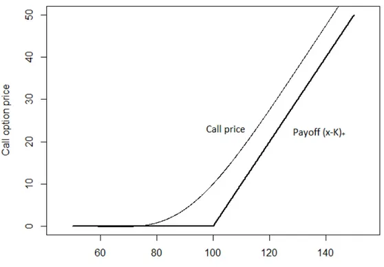
Figure 4.2: Black-Scholes pricing of a call option at time t=0, with K =100,

T =2, r=0.04 and s =0.1.

call options. Hence, for the following, we assume that either h is bounded or h(x) = (x K)+.

Now, let f be a replicating strategy for H. Such a strategy exists by theorem 4.13. By Theorem 4.12, P(t, St) is equal to the value of the strategy Vf(t):

ertf1_t +f2_tSt =P(t, St) (4.28)

Differentiating on both sides, and applying the self-financing condition on the left side, we obtain:

(rertf_t1+f2_tµSt)dt+f2tsStdWt = (Pt+µStPx+1₂s2St2Pxx)dt+sStPxdWt

(4.29) Where all the partial derivatives of P are evaluated at (t, St) - we will use

this abbreviation later on without further mention. By the uniqueness of the expression of an Itô process, we conclude that:

f2_t =Px(t, St) (4.30)

And from 4.28 we deduce that:

f_t1=e rt(P(t, St) Px(t, St)St) (4.31)

The previous argument also shows the relationship between the pricing func-tion P(t, x) and a certain PDE (the Black-Scholes PDE). Indeed, substituting

the value of the hedging strategy in 4.29, we obtain the formula: