To Ackermann-ize or not to Ackermann-ize? On Efficiently Handling Uninterpreted Function Symbols in SMT(EUF U T)

UNIVERSITY

OF TRENTO

DEPARTMENT OF INFORMATION AND COMMUNICATION TECHNOLOGY

38050 Povo – Trento (Italy), Via Sommarive 14

http://www.dit.unitn.it

TO ACKERMANN-IZE OR NOT TO ACKERMANN-IZE?

ON EFFICIENTLY HANDLING UNINTERPRETED FUNCTION

SYMBOLS IN SMT (EUF U T)

Roberto Bruttomesso, Alessandro Cimatti, Anders Franzén

Alberto Griggio, Alessandro Santuari, and Roberto Sebastiani

May 2006

To Ackermann-ize or not to Ackermann-ize?

On Efficiently Handling Uninterpreted Function

Symbols in SMT(

EUF

∪

T

)

Roberto Bruttomesso1_{, Alessandro Cimatti}1_{, Anders Franz´en}1,2_,

Alberto Griggio2_{, Alessandro Santuari}2_{, and Roberto Sebastiani}2

1_{ITC-IRST, Povo, Trento, Italy.{bruttomesso,cimatti,franzen}@itc.it}

2_{DIT, Universit`a di Trento, Italy.{griggio,santuari,rseba}@dit.unitn.it}

Abstract. Satisfiability Modulo Theories (SMT(T)) is the problem of deciding

the satisfiability of a formula with respect to a given background theoryT. When T is the combination of two simpler theoriesT1andT2(SMT(T1∪T2)), a

stan-dard and general approach is to handle the integration ofT1andT2by performing

some form of search on the equalities between the shared variables.

A frequent and very relevant sub-case of SMT(T1∪T2) is whenT1 is the

the-ory of Equality and Uninterpreted Functions (EUF). For this case, an alterna-tive approach is to eliminate first all uninterpreted function symbols by means of Ackermann’s expansion, and then to solve the resulting SMT (T2) problem.

In this paper we build on the empirical observation that there is no absolute win-ner between these two alternative approaches, and that the performance gaps be-tween them are often dramatic, in either direction.

We propose a simple technique for estimating a priori the costs and benefits, in terms of the size of the search space of an SMT tool, of applying Ackermann’s expansion to all or part of the function symbols. We have implemented a prepro-cessor which analyzes the input formula, decides autonomously which functions to expand, performs such expansions and gives the resulting formula as input to an SMT tool.

A thorough experimental analysis, including the benchmarks of the SMT’05 com-petition, shows that our preprocessor performs the best choice(s) nearly always, and that the proposed technique is extremely effective in improving the overall performance of the SMT tool.

1 Introduction

Satisfiability Modulo a Theory

T

(SMT(

T

)) is the problem of checking the satisfiabil-ity of a quantifier-free (or ground) first-order formula with respect to a given first-order theory

T

.1_{Theories of interest for many applications are, e.g., the theory of difference}

logic

DL

, the theory

EUF

of equality and uninterpreted functions, the quantifier-free

fragment of Linear Arithmetic over the rationals

LA

(Q) and that over the integers

LA

(Z), the theory of bit-vectors

BV

. A prominent approach to SMT(

T

), which

un-derlies several systems (e.g., CVCLITE[3], DLSAT [11], DPLL(T)/BarceLogic [13],

MATHSAT [6], TSAT++ [2], ICS/YICES[12]), is based on extensions of propositional

SAT technology: a SAT solver is modified to enumerate boolean assignments, and inte-grated with a decision procedure for sets of literals in the theory

T

(

T

-solver).

When

T

is the combination of two simpler theories

T

1and

T

2(SMT(

T

1∪

T

2)), a

standard and general approach is to handle the integration of

T

1and

T

2by performing

some form of search on the equalities between the variables which are shared between the theories (interface equalities): in the Nelson-Oppen [14] and Shostak [16] schemata (NO hereafter), the interface equalities are deduced by the

T

-solvers; in the Delayed

Theory Combination schema (DTC hereafter) [8, 9] all or part of them are assigned to truth values also by the underlying SAT solver.

A frequent and very relevant sub-case is when one of the two theories is that of equality and uninterpreted functions

EUF

. (Hereafter we refer to this problem as SMT (

EUF

∪

T

).) For this case, an alternative approach is to eliminate first all uninterpreted function symbols by means of Ackermann’s expansion [1], and then to solve the result-ing sresult-ingle-theory SMT(

T

) problem. (Hereafter we refer to this approach as ACK.)

In this paper we focus on SMT (

EUF

∪

T

). Comparing the performances of DTC

and ACKapproaches, we notice that not only there is no absolute winner, but also the

performance gaps are often dramatic, in either direction. We investigate the causes of this fact, and we introduce a technique for estimating off-line the costs and benefits, in terms of the size of the search space of an SMT tool, of applying Ackermann’s expan-sion to all or part of the function symbols.

We have implemented a preprocessor which analyzes the input formula, decides autonomously which functions to expand, performs such expansions and gives the re-sulting formula as input to an SMT tool.

A thorough experimental analysis, including the benchmarks of the SMT’05 com-petition, shows that our preprocessor performs the best choice(s) nearly always, and that the proposed technique is extremely effective in improving the overall performance of the SMT tool.

The paper is organized as follows. In §2 we introduce the necessary background

in-formation on SMT, SMT(

T

1∪

T

2), DTC and Ackermann’s expansion. In §3 we present

the main intuitions and ideas underlying our work. In §4 we present our new preproces-sor. In §5 we present the experimental evaluation of our work. In §6 we conclude and briefly present potential future developments.

2 Background

2.1 Satisfiability Modulo Theory

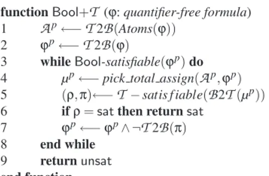
Fig. 1 presents Bool+

T

, (a much simplified version of) a standard schema of a decision

procedure for SMT(

T

). The function Atoms(ϕ) takes a ground formula ϕ and returns

the set of atoms which occur in ϕ. We use the notation ϕp_{to denote the propositional}

ab-straction of ϕ, which is formed by the function

T

2

B

that maps propositional variables to themselves, ground atoms into fresh propositional variables, and is homomorphic w.r.t. boolean operators and set inclusion. The function

B

2

T

is the inverse of

T

2

B

. We use µpto denote a propositional assignment, i.e. a conjunction (a set) of propositional literals. (If

T

2

B

(µ) |=

T

2

B

(ϕ), then we say that µ propositionally satisfies ϕ.)

function Bool+T (ϕ: quantifier-free formula)

1 Ap_{←−T2B(Atoms(ϕ))}

2 ϕp_{←−T2B(ϕ)}

3 while Bool-satisfiable(ϕp_{) do}

4 µp_{←− pick total assign(A}p_{, ϕ}p₎

5 (ρ, π)←−T− satis f iable(B2T(µp))

6 if ρ = sat then return sat

7 ϕp←− ϕp∧ ¬T2B(π)

8 end while

9 return unsat

end function

Fig. 1. A simplified view of enumeration-based T-satisfiability procedure: Bool+T

The idea underlying the algorithm is that the truth assignments for the propositional abstraction of ϕ are enumerated and checked for satisfiability in

T

. The procedure ei-ther returns sat if one such model is found, or returns unsat oei-therwise. The function

pick total assign returns a total assignment to the propositional variables in ϕp_{, that is,}

it assigns a truth value to all variables in

A

p_{. The function}

_T

_{-satisfiable(µ) detects if the}

set of conjuncts µ is

T

-satisfiable: if so, it returns (sat, /0); otherwise, it returns (unsat, π), where π ⊆ µ is a

T

-unsatisfiable set, called a theory conflict set. We call the negation of a conflict set, a conflict clause.

The algorithm is a coarse abstraction of the ones underlying most SMT tools

(includ-ing, e.g., TSAT++, MATHSAT, DLSAT, DPLL(T)/BarceLogic, CVCLITE, ICS/YICES).

In practice, the enumeration is carried out by means of efficient implementations of the DPLL algorithm [17], where a partial assignment µp_{is built incrementally, and}

unit propagation is used extensively to perform all the assignments which derive

de-terministically from the current µp_{. Conflict sets, generated because either the current}

µp_{falsifies the formula or because}

_T

_{-satisfiable(}

_B

₂

_T

_(µp_{)) fails, are used to prune the}

search tree and to backtrack as high as possible (backjumping), and learned as conflict clauses to avoid generating the same conflicts in future branches. Another important im-provement is early pruning: intermediate assignments are checked for

T

-satisfiability and, if not

T

-satisfiable, then are pruned (since no refinement can be

T

-satisfiable); finally, theory deduction can be used to reduce the search space by explicitly returning truth values for unassigned literals, as well as constructing/learning implications. The interested reader is pointed to [6, 7] for details and further references.

2.2 SMT(T1∪ T2) via theory combination

In many practical applications of SMT(

T

), the background theory is a combination

of two (or more) theories

T

1 and

T

2. Most approaches to SMT(

T

1∪

T

2) rely on the

adaptation of the Bool+

T

schema, by instantiating

T

-satisfiable with some decision

procedure for the satisfiability of

T

1∪

T

2, typically based on an integration schema like

Nelson-Oppen (NO) [14] (or its variant due to Shostak [16]), or on the more recent Delayed Theory Combination (DTC) schema [5, 9].

Both the NO and DTC schemata work only for combinations of stably-infinite and

signature-disjoint theories

T

iwith equality (we recall that

T

iis stably-infinite iff every

function DTC (ϕi: quantifier-free formula)

1 ϕ ←− purify(ϕi)

2 Ap_{←−T2B(Atoms(ϕ) ∪ interface equalities(ϕ))}

3 ϕp_{←−T2B(ϕ)}

4 while Bool-satisfiable (ϕp_{) do}

5 µp₁∧ µp₂∧ µep= µp←− pick total assign(Ap, ϕp)

6 (ρ1, π1)←−T1-satisfiable (B2T(µ1p∧ µpe))

7 (ρ2, π2)←−T2-satisfiable (B2T(µ₂p∧ µpe))

8 if (ρ1= sat ∧ ρ2= sat) then return sat else

9 if ρ1= unsat then ϕp←− ϕp∧ ¬T2B(π1)

10 if ρ2= unsat then ϕp←− ϕp∧ ¬T2B(π2)

11 end while

12 return unsat

end function

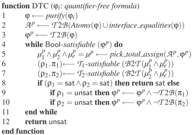
Fig. 2. A simplified view of the DTC procedure for SMT(T1∪T2)

they require the input formula to be pure: a formula ϕ is pure iff every atom ψ in ϕ is

i-pure for some i ∈ {1, 2}, that is ψ contains only =, variables and symbols from the

signature of

T

i. Every non-pure

T

1∪

T

2formula ϕ can be converted into an equivalently

satisfiable pure formula ϕ0 _{by recursively labeling terms t with fresh variables v} t, and

by conjoining the definition atom (vt= t) to the formula. E.g.:

( f (x+3y) = g(2x−y)) =⇒ ( f (vx+3y) = g(v2x−y))∧(vx+3y= x+3y)∧(v2x−y= 2x−y).

This process is called purification, and is linear in the size of the input formula. In a pure formula ϕ, an interface variable is a variable appearing in both 1-pure and 2-pure atoms. An interface equality is an equality between two interface variables.

In the NO schema, the two decision procedures for

T

1 and

T

2(

T

i-solvers)

coop-erate by exchanging (disjunctions of) interface equalities (ei j’s). In the DTC schema,

each of the two

T

i-solvers works in isolation, without direct exchange of information.

Their mutual consistency is ensured by augmenting the input problem with all interface equalities ei j, even if these do not occur in the original problem. The enumeration of

assignments includes not only the atoms in the formula, but also the interface equalities

ei j. Both theory solvers receive, from the boolean level, the same truth assignment µefor

ei j: under such conditions, the two “partial” models found by each decision procedure

can be merged into a model for the input formula.

A simplified view of the DTC algorithm is presented in Fig. 2. Initially (lines 1–3), the formula is purified, the ei j’s which do not occur in the purified formula are created

and added to the set of propositional symbols

A

p_{, and the propositional abstraction ϕ}p

of ϕ is created. Then, the main loop is entered (lines 4–11): while ϕp_{is propositionally}

satisfiable (line 4), a satisfying truth assignment µp_{is selected (line 5). Truth values}

are associated not only to atoms in ϕ, but also to the ei j atoms, even though they do

not occur in ϕ. µp _{is then (implicitly) separated into µ}p

1∧ µep∧ µp2, where

B

2

T

(µip) is

a set of i-pure literals and

B

2

T

(µep) is a set of ei j-literals. The relevant part of µpare

checked for consistency against each theory (lines 6–7);

T

i-satisfiable(µ) returns a pair

(ρi, πi), where ρiis unsat iff µ is unsatisfiable in

T

i, and sat otherwise. If both calls to

T

i

-satisfiable return sat, then the formula is -satisfiable. Otherwise, when ρiis unsat, then

to exclude truth assignments which may fail in the same way (line 9–10), and the loop is resumed. Unsatisfiability is returned (line 12) when the loop is exited without having found a model.

In practical implementations of DTC, as before, the enumeration is carried out by means of efficient implementations of the DPLL engine, where a partial assignment

µp_{is built incrementally, exploiting unit-propagation, backjumping and learning, early}

pruning, theory deduction. Moreover, if one or both

T

i-satisfiable have the capability of

deducing (disjunctions of) interface equalities which derive in

T

ifrom a partial

assign-ment µ,2_{then such a deduction is exploited to prune the boolean search on the interface}

equalities (ei j-deduction). To this extent, DTC extends the NO schema, in the sense that

it allows for using

T

i-satisfiable procedures with every deduction capability, trading ei j

-deduction power with boolean search, and allows for emulating the NO schema [10]. For the sake of simplicity, in this paper we do not consider ei j-deduction for DTC. We

refer the reader to [9, 10] for a more detailed discussion.

Example 1. Let ϕ be the following

EUF

∪

LA

(Z)-pure formula

ϕ ≡ w = h(x) ∧ a = h(y) ∧ c = f (z) ∧ d = f (b) ∧ f (c) = f (b) ∧

w = f (d) ∧ ¬(c = d) ∧ x ≥ y ∧ x ≤ y ∧ z = w − a ∧ b = 0. (1) x, y, z, w, a, b are the interface variables, so that there are 15 interface equalities: z = b, w = b, a = b, x = b, y = b, z = w, z = a, x = z, y = z, w = a, x = w, y = w, x = a, y = a, x = y.

The DPLL solver generates first the assignment µ := µEUF ∪ µLA(Z)satisfying ϕ, s.t.

µEUF := {w = h(x), a = h(y), c = f (z), d = f (b), f (c) = f (b), w = f (d), ¬(c = d)},

µLA(Z):= {x ≥ y, x ≤ y, z = w − a, b = 0}.

Then it tries to extend it with a total truth assignment µeto the interface equalities such

that µEUF ∪ µeand µLA(Z)∪ µeare consistent in

EUF

and

LA

(Z) respectively. This

requires some search on the 15 interface equalities.

E.g, if the DPLL engine is smart or lucky enough to select first x = y, w = a, z = b, then we have

µLA(Z)∪ {¬(x = y)} |=LA(Z)⊥, so that x = y is added to µ,

µEUF∪ {x = y, ¬(w = a)} |=EUF ⊥, so that w = a is added to µ,

µLA(Z)∪ {x = y, w = a, ¬(z = b)} |=LA(Z)⊥, so that z = b is added to µ,

µEUF∪ {x = y, w = a, z = b} |=EUF ⊥, hence ϕ is

EUF

∪

LA

(Z)-inconsistent. ¦

Notice that on a single-theory SMT(

T

) problem, DTC behaves as a standard SMT

tool, because there are no interface equalities.

2.3 SMT(

EUF

∪

T

) via Ackermann’s expansion

When one of the theories

T

iis

EUF

, another possible approach to the SMT(

T

1∪

T

2)

problem is to eliminate uninterpreted function symbols by means of Ackermann’s

ex-pansion [1] so to obtain an SMT(

T

) problem with only one theory. The method works

by replacing every function application occurring in the input formula ϕ with a fresh

variable and then adding to ϕ all the needed functional consistency constraints. The new formula ϕ0_{obtained is equisatisfiable with ϕ, and contains no uninterpreted}

func-tion symbols. First, each distinct funcfunc-tion applicafunc-tion f (x1, . . . , xn) is replaced by a fresh

variable vf (x1,...,xn). Then, for every pair of distinct applications of the same function,

f (x1, . . . , xn) and f (y1, . . . , yn), a constraint

(

arity( f )_^ i=1

ack(xi) = ack(yi)) → vf (x1,...,xn)= vf (y1,...,yn), (2)

is added, where ack is a function that maps each function application g(z1, . . . , zn) into

the corresponding variable vg(z1,...,zn), each variable into itself and is homomorphic wrt.

the interpreted symbols. The atom ack(xi) = ack(yi) is not added if the two sides of the

equality are syntactically identical.

Example 2. Let ϕ be the pure formula (1) of Example 1. Then, replacing every function application with a fresh variable, and adding all the functional consistency constraints, we obtain the formula

ϕACK ≡ w = vh(x)∧ a = vh(y)∧ c = vf (z)∧ d = vf (b)∧ vf (c)= vf (b)∧ w = v_{f (d)}∧ ¬(c = d) ∧ x ≥ y ∧ x ≤ y ∧ z = w − a ∧ b = 0 ∧ (x = y → vh(x)= vh(y)) ∧ (z = b → vf (z)= vf (b)) ∧ (z = c → vf (z)= vf (c)) ∧ (z = d → vf (z)= vf (d)) ∧ (c = b → v_{f (c)}= v_{f (b)}) ∧ (c = d → v_{f (c)}= v_{f (d)}) ∧ (b = d → vf (b)= vf (d)). (3)

The DPLL solver first deterministically selects the truth assignment

µ_LA(Z):= { w = vh(x), a = vh(y), c = vf (z), d = vf (b), vf (c)= vf (b), w = vf (d),

¬(c = d), x ≥ y, x ≤ y, z = w − a, b = 0} ,

which is consistent in

LA

(Z). Then, it performs some search on the remaining 12

equalities.3

E.g., if it is smart or lucky enough to select first x = y, z = b, then we have:

µLA(Z)∪ {¬(x = y)} |=LA(Z)⊥, so that x = y is added to µ,

µLA(Z)∪ {x = y, vh(x)= vh(y), ¬(z = b)} |=LA(Z)⊥, so that z = b is added to µ,

µ_LA(Z)∪{x = y, vh(x)= vh(y), z = b, vf (z)= vf (b)} |=LA(Z)⊥, hence ϕ is

EUF

∪

LA

(Z)-inconsistent. ¦

Notice that, for simplicity, in Example 1 we have considered a pure formula ϕ, which might be the result of purifying some non-pure formula ϕ0_{. If so, applying}

Ack-ermann expansion directly to ϕ0might result into a more compact formula than (3). Henceforth, we call respectively Ackermann constraints or Ackermann

implica-tions the functional consistency constraints added by Ackermann expansion, Acker-mann equalities the equalities occurring in the AckerAcker-mann constraints, and AckerAcker-mann variables the variables occurring in the Ackermann equalities.

3_{The remaining equalities are only 12 because v}

f (c)= vf (b)causes the removal of the 5th

Wisa Hash D T C 0.1 1 10 100 1000 10000 0.1 1 10 100 1000 10000 D T C 0.1 1 10 100 1000 10000 0.1 1 10 100 1000 10000 ACK ACK

Fig. 3. Execution time ratio (in logarithmic scale) for DTC and ACKon the benchmarks Wisa

and Hash, using MATHSAT. A dot above the diagonal line means better performance of ACK

and vice versa. The horizontal and vertical dashed lines represent time-out.

3 To Ackermann-ize or not to Ackermann-ize?

We start from a simple empirical observation: neither DTC or ACKalways prevails in

the task of solving SMT(

EUF

∪

T

) problems, and the performance gaps between the

two approaches may be dramatic, in either direction. As an example, Figure 3 shows the execution times of the two approaches on two different groups of benchmarks, for the MATHSAT [7] solver (both tests will be described in §5). For the Wisa benchmarks

(left), ACK is up to 1000 times4 _{faster than DTC, whilst for the Hash benchmarks}

(right) the converse is true.

By tracing the behavior of MATHSAT on these tests, we notice that the performance gaps mirror the different amount of boolean search performed by the two techniques. From which we argue that one of the main reasons of such big performance gaps is the different size of the boolean search space that each technique has to explore in order to decide the satisfiability of its input.

Thus, we look to both techniques from the perspective of the boolean search only.

Both DTC and ACK require the SAT solver to perform an extra boolean search on

equalities which did not occur in the original formula (i.e., on the interface equalities and on the Ackermann equalities respectively). Thus the enlargement of the boolean search space with the two techniques depends directly to the number of these new equal-ities introduced.

3.1 Enlargement of the search space with DTC

In the DTC approach it may necessary to assign a truth value to up to all the interface equalities. If ϕ is a pure

EUF

∪

T

formula, then the number of interface equalities is given by

|

V

| · (|

V

| − 1)

2 ,

where |

V

| is the number of interface variables in ϕ. (Notice that this is an upper bound

for the number of the new equalities introduced, since some of them might already appear in ϕ.) Thus, with DTC, the number of boolean atoms the SAT solver may have to explore is enlarged by a factor that is quadratic in the number of the interface variables. Example 3. The formula ϕ of Example 1 has 6 interface variables, so that the number of atoms the SAT solver may have to explore is increased by (6 · 5)/2 = 15 interface

equalities, all of which are new. ¦

Notice that, in general, the input problem ϕ must be purified to be handled by DTC. The purification process adds a number of new variables and atoms that is linear in the size of ϕ. However, this does not cause an enlargement of the boolean search space, because all the atoms added are definitions of terms like (vt = t) and occur as unit

clauses in the resulting formula, so that they are assigned a priori and deterministically to true by the SAT solver.

3.2 Enlargement of the search space with ACK

In the ACKapproach, the increase in the boolean search space depends on the number

of (new) equalities in the Ackermann constraints introduced.

Let

F

be the set of (distinct) function symbols occurring in ϕ, and let

O

f be the set

of all (distinct) applications of the function f in the input formula ϕ. Then the number of new Ackermann equalities introduced is less or equal than

∑

f ∈F

|

O

f| · (|

O

f| − 1)

2 · (arity( f ) + 1). (4)

In fact, for each f ∈

F

and for each of the (|

O

f| · (|

O

f| − 1))/2 pairs of distinct

occur-rences of f , Equation (2) causes the introduction of up to (arity( f ) + 1) new Ackermann equalities. (As with DTC, this is an upper bound, both because some of the equalities in one constraint could already occur in the formula or in other constraints, and because identities like x = x are dropped by construction.)

Thus, with ACK, the number of boolean atoms the SAT solver may have to explore

is enlarged by a factor that is quadratic in the number of occurrences of each function symbol, and linear in the number of distinct function symbols and in their arity. Example 4. In the formula ϕ (1) of Example 1,

O

h= 1 and

O

f= 4. Thus the Ackermann

constraints introduced in the formula ϕACK(3) of Example 2 contain (2·1)/2·(1+1)+

(4 · 3)/2 · (1 + 1) = 14 equalities. Since v_{f (c)}= v_{f (b)}is not new, the new equalities are 13. Notice that also c = b does not really increase the boolean search space, because the

5th implication is immediately removed by the DPLL solver (Footnote 3). ¦

3.3 Intuition: the “frontier” between

EUF

and

T

in DTC and ACK

Both DTC and ACKintroduce an enlargement of the search space of the input problem

ϕ. Intuitively, we can think of this extra boolean search as the cost associated to each of the two approaches for handling the interaction between the two theories. We notice

T

f

f

g

g

T

f

f

g

g

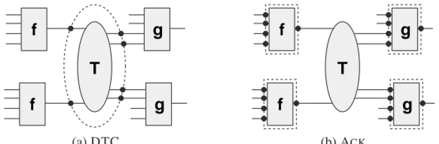
(a) DTC (b) ACK

Fig. 4. Schemas of the frontier betweenEUF andT in the DTC and ACKapproaches.

function DECIDE(ϕ: quantifier-free formula)

1 ack eq ←− countAckEqualities(ϕ)

2 int eq ←− countInterfaceEqualities(ϕ)

3 if ack eq < int eq then

4 return ackermanize(ϕ)

5 else

6 return ϕ

7 end if

end function

Fig. 5. High-level description of the DECIDEalgorithm

that the set of new equivalences introduced by either approach corresponds to a distinct

notion of “frontier” between

EUF

and

T

in the two approaches.

In DTC, the frontier is given by the interface variables (see Figure 4.a). As the cost of DTC depends quadratically on the size of the frontier, DTC is expected to perform better for those examples where the two theories are loosely coupled, and worse when there is a strong connection between them.

With ACK, the frontier between the two theories is potentially much larger, because

it consists in the inputs and outputs of all (distinct) function applications (i.e, the Acker-mann variables), including those which do not interact with terms of the theory

T

(see Figure 4.b). However, in this case the cost is not quadratic on the number of variables in the frontier; rather, it depends on the number of different functions and of distinct

occurrences of each function invocation (4). Thus ACK is expected to perform better

when the number of distinct function invocations for the same function is low.

4 Cost-driven Ackermann-ization

When we want to check the satisfiability of an SMT(

EUF

∪

T

) formula ϕ, no matter

which of the two approaches (DTC or ACK) we use, we must pay a price in terms

of enlargement of the boolean search space. We believe that this cost is one of the main factors which influence the performance of the two methods. Thus, being able to estimate this cost a priori can drive the choice of which technique to apply.

4.1 A global-decision approach: DECIDE

Our first, basic idea is that of trying to estimate a priori the difference of costs of

first idea “a global-decision approach” because here the decision involves all function symbols altogether.

The resulting algorithm DECIDEis outlined in Figure 5. Let ϕ be a (possibly

non-pure) SMT(

EUF

∪

T

) formula. The function countAckEqualities returns the number

of new Ackermann equalities added by the Ackermann’s expansion of ϕ. The func-tion countInterfaceEqualities returns the number of new interface equalities in (the for-mula resulting from purifying) ϕ. Notice that both functions return the exact number of equalities introduced, avoiding counting repeated equalities, identities x = x, etc. Both functions are straightforward to implement, and their complexity is linear in the size of ϕ.

DECIDE works as a preprocessor for an SMT solver for SMT(

EUF

∪

T

) which

uses DTC: the algorithm either returns an Ackermann-ized version of the input ϕ (if ACKcosts less), or leaves the input untouched. As noticed in §2, in the first case DTC

behaves as a standard single-theory SMT tool, so that the two options correspond to

ACKand DTC respectively.

Example 5. Consider again the formulas (1) and (3) of Examples 1 and 2 respectively.

DTC would introduce 15 new interface equalities, whilst ACKwould introduce 13 new

Ackermann equalities. Therefore DECIDEin this case would choose ACK.

4.2 A local-decision approach: PARTIAL

The idea just described can be generalized in the following way. From §3 we know that the cost of DTC depends quadratically on the global number of interface variables, whilst the cost of ACK, for each function symbol f , depends quadratically on the

num-ber of the distinct occurrences of f and linearly on its arity. Thus, we can decide to apply Ackermann’s expansions only to subsets of the function symbols, according to their relative costs. We call this second idea “a local-decision approach” because here the decision involves subsets of function symbols.

Let f be a function in ϕ with very few occurrences but many arguments shared be-tween

EUF

and

T

. Then f causes a low increase of the ACKcosts and a big increase of the DTC costs, because Ackermann’s expansion will introduce few constraints, whilst the high number of interface variables would make DTC generate many new equalities. On the other hand, a function g with many occurrences but few or no arguments shared among the theories is going to cost much less for DTC than for ACKfor the very same reason. Thus, if we consider a formula which contains both f and g, then applying Ack-ermann’s expansion only partially, so that to remove only f , and solving the resulting

problem with DTC, is going to cost less than pure ACKor pure DTC.

Example 6. Consider again the formula (1) of Example 1. If we expand only h, we get the following formula:

ϕ0 _{≡ w = v}

h(x)∧ c = f (z) ∧ d = f (b) ∧ f (c) = f (b) ∧ w = f (d) ∧

¬(c = d) ∧ x ≥ y ∧ x ≤ y ∧ z = w − vh(y)∧ b = 0 ∧

x = y → vh(x)= vh(y),

(5)

which has only 3 interface variables (z, b and w). Using DTC on ϕ0 would then

function PARTIAL(ϕ: quantifier-free formula) 1 A←− /0 2 ψ ←− puri f y(ϕ) 3 do 4 B←− selectFunctionsToAckermanize(ψ) 5 ψ ←− ackermanizeFunctions(ψ,B) 6 A←−A∪B 7 whileB6= /0 8 ϕ0_{←− ackermanizeFunctions(ϕ,A)} 9 return ϕ0 end function

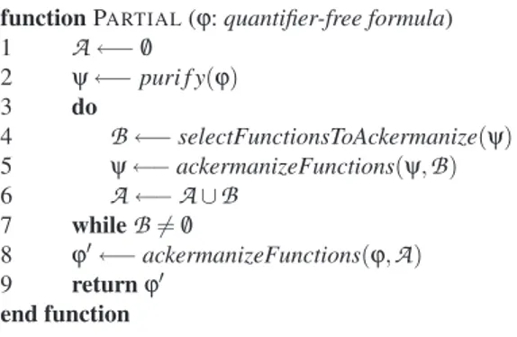
Fig. 6. High-level description of the PARTIALalgorithm

cost in total 5 new equalities (2 for the Ackermann constraints and 3 for the interface

equalities), which is less than with ACK(13) and DTC (15). ¦

The ideal solution would be to develop an algorithm that applies Ackermann’s ex-pansion to the subset of the function symbols corresponding to a global minimum in the number of new equalities to add. Unfortunately, finding such a global optimal solution seems to be very expensive. Intuitively, this is because both the cost and the bene-fit of applying Ackermann’s expansion to each function symbol —in terms of more Ackermann equalities and less interface equalities to add respectively— depend on the previous eliminations of some other functions. (For example, as a consequence of the elimination of a function f , it may become convenient to eliminate also g because they had many pairs of corresponding arguments in common.) Thus, finding the global opti-mum may require exploring up to all the 2|F|_{possible subsets of function symbols.}

For this reason, we have conceived instead the algorithm PARTIAL(outlined in

Fig-ure 6) which finds a local optimum. PARTIALis a greedy algorithm that starts from the

purified formula and that finds at each step a set of function symbols

B

whose removal causes a reduction in the number of equivalences to add. When this set is empty, a local minimum has been reached, and the algorithm terminates. Then the Ackermann’s ex-pansion on the set of selected functions

A

is performed on the original input formula ϕ, and the result is returned.

The core of PARTIALis the function selectFunctionsToAckermanize, which returns

the set of functions to remove in order to reduce the number of new equalities to add, according to the following heuristic. The function symbols occurring in ϕ are divided into (possibly overlapping) subgroups

G

v’s, one for every interface variable v in ϕ,

G

v

consisting in the set of all the function symbols that cause v to be an interface vari-able. Then it is returned the group

G

vwhich causes the maximum reduction gainGv in

terms of equivalences to add. (That is, gain_Gv is defined as the difference between the number of interface equalities to remove and the number of equalities in the functional consistency constraints to add, if all the functions in the group were removed with Ack-ermann’s expansion.) If for no group

G

vthe value gainGv is positive, then the empty set

is returned.5

5_{As a direct consequence of how the groups are built, removing the functions in a group removes}

Example 7. Consider the pure formula (1) used in all the previous examples. When invoked for the first time, selectFunctionsToAckermanize constructs for the set of func-tions { f , h} in (1) six groups, one for each interface variable:

G

x=

G

y=

G

a= {h}

G

w=

G

z=

G

b= { f }.

Then, for each of them, the associated gain (i.e. the difference between the number of interface equalities to remove and the number of equalities to add for the functional consistency constraints) is computed:

gainGx= gainGy= gainGa = 12 − 2 = 10, gainGw= gainGz= gainGb = 12 − 11 = 1

because removing h makes x, y and a loose the status of interface variables, whilst re-moving f the same happens for w, z and b. Thus selectFunctionsToAckermanize selects

{h} only, causing the generation of the formula (5) of Example 6. At the next iteration

of the main loop of PARTIAL, the only function symbol is f , which is not removed since

all gainGv’s are negative. ¦

5 Empirical Evaluation

We implemented both DECIDE and PARTIAL in a preprocessor program, written in

C++. It handles SMT(

EUF

∪

LA

) problems, and has four different operational modes:

transparent (DTC), which simply reads a problem from its standard input (in either MATHSAT or SMT [15] format) and outputs it to its standard output without doing anything;

ackermanize, which removes every uninterpreted function symbol;

decide, which applies the DECIDEalgorithm; and

partial, which applies the PARTIALalgorithm to remove a subset of the uninterpreted

function symbols.

We tested our preprocessor with the MATHSAT [7] solver, which handles SMT(

EUF

∪

LA

) problems with DTC. We used different benchmark suites, coming from different

domains:

QF UFIDL comes from the SMT-LIB [15], and is made of formulas with

EUF

and integer difference logic. It is a superset of the QF UFIDL set used in the SMT-COMP’05 competition [4];

Wisa are software verification benchmarks from the Wisconsin Safety Analyzer,

cre-ated with a slightly modified version of the generator available at http://www.cs. wisc.edu/wisa/papers/icse05/wisa-benchmarks.html;

EufLaArithmetic are simulations of arithmetic operations (succ, pred, sum) modulo

N, using

EUF

and

LA

(Z). This and the following groups of benchmarks were

introduced in [9];

Hash are problems over hash tables, modeled with a combination of

EUF

and

LA

(Z);

It may be the case that more than one interface variable is removed: e.g., ifGx⊆Gy, then

RandomCoupled are randomly generated SMT(

EUF

∪

LA

(Q)) problems, with a propositional 3-CNF structure. In this group, there is a high coupling between the two theories, that is there is a high probability that for instance an argument of a function is a

LA

(Q) term;

RandomDecoupled are tests generated in the same way as the previous group, but

where the coupling between

EUF

and

LA

(Q) is low.

The tests were run on a machine with an Intel Xeon 3GHz processor running Linux.

The memory limit was set to 1GB, and the time limit to 1000 sec. 6

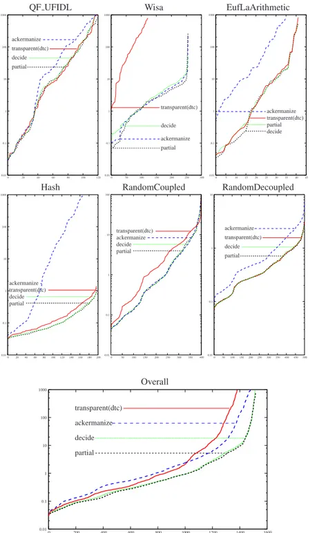
Figure 7 shows the results, both for the individual suites singularly and for the union of all the suites. A point in hX,Y i states that X problems have been solved each in less or equal than Y seconds. (Notice the logarithmic scale of the Y axis.) A higher number of tests solved means better performance. When this number is the same, the lowest line is the best.

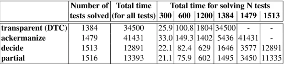
The following table summarizes the total results. The rows are sorted from the worst to the best, while the columns show details of the performances in terms of total number of tests solved, total running time, and total time to solve a fixed amount N of tests, for various values of N.

Number of Total time Total time for solving N tests tests solved (for all tests) 300 600 1200 1384 1479 1513 transparent (DTC) 1384 34500 25.9 100.8 1804 34500 - -ackermanize 1479 41431 33.0 149.3 1402 5436 41431 -decide 1513 12891 22.1 82.4 629 1646 3577 12891 partial 1516 13393 21.1 75.9 602 1495 3450 11335

We can see from both Figure 7 and the above table that different suites show very

different performance gaps between transparent (DTC) and ackermanize (ACK), as

observed in §2, and that both decide (DECIDE) and partial (PARTIAL) always behave

quite similarly to the best of the two. (E.g., looking at the data, we noticed that decide chooses the most efficient option nearly always, and that the few samples for which it

does not are such that the performance gaps between ACKand DTC are minor.)

The overall result shows that both DECIDEand PARTIALare globally much more

efficient than both ACKand DTC, with PARTIALbeing the best technique.

6 Conclusions

In this paper we have focused on the SMT(

EUF

∪

T

) problem. We have proposed a

simple technique for estimating a priori the costs and benefits, in terms of the size of the search space of an SMT tool, of applying Ackermann’s expansion to all or part of the function symbols; we have implemented a preprocessor which analyzes the input formula, decides autonomously which functions to expand, performs such expansions and gives the resulting formula as input to an SMT tool; we have performed a thorough

experimental analysis with MATHSAT on SMT(

EUF

∪

DL

), SMT(

EUF

∪

LA

(Q))

6_{In order to make the results reproducible, the binaries of the tools used and the benchmarks}

QF UFIDL Wisa EufLaArithmetic 0.01 0.1 1 10 100 1000 0 20 40 60 80 100 120 ackermanize transparent(dtc) decide partial 0.01 0.1 1 10 100 1000 0 50 100 150 200 250 300 transparent(dtc) decide ackermanize partial ackermanize transparent(dtc) partial decide 0.01 0.1 1 10 100 1000 0 5 10 15 20 25 30 35 40 45

Hash RandomCoupled RandomDecoupled

ackermanize transparent(dtc) decide partial 0.01 0.1 1 10 100 1000 0 20 40 60 80 100 120 140 160 180 200 transparent(dtc) ackermanize decide partial 0.01 0.1 1 10 100 0 50 100 150 200 250 300 350 400 0.01 0.1 1 10 0 50 100 150 200 250 300 350 400 450 500 ackermanize transparent(dtc) decide partial Overall 0.01 0.1 1 10 100 1000 0 200 400 600 800 1000 1200 1400 1600 transparent(dtc) ackermanize decide partial

Fig. 7. Results of the benchmarks for the MATHSAT solver. For each technique, the X axis

rep-resents the number of tests solved and the Y axis the time required (in log scale). The labels in the plots are sorted according to performance: from the worst to the best.

and SMT(

EUF

∪

LA

(Z)), showing that the proposed technique is extremely effective in improving the overall performance of the SMT tool.

As future developments, we plan to experiment the effectiveness of our techniques also with other SMT tools (e.g., CVCLITE[3], ICS/YICES[12]), and with other theo-ries (e.g.,

EUF

with the theory of bit-vectors

BV

).

References

1. W. Ackermann. Solvable Cases of the Decision Problem. North Holland Pub. Co., 1954.

2. A. Armando, C. Castellini, E. Giunchiglia, and M. Maratea. A SAT-based Decision Proce-dure for the Boolean Combination of Difference Constraints. In Proc. SAT’04, 2004.

3. C.L. Barrett and S. Berezin. CVC Lite: A New Implementation of the Cooperating Validity Checker. In Proc. CAV’04, volume 3114 of LNCS. Springer, 2004.

4. Clark Barrett, Leonardo de Moura, and Aaron Stump. SMT-COMP: Satisfiability modulo theories competition. In CAV ’05, volume 3576 of LNCS, pages 20–23. Springer-Verlag, 2005.

5. M. Bozzano, R. Bruttomesso, A. Cimatti, T. Junttila, P.van Rossum, S. Ranise, and R. Sebas-tiani. Efficient Satisfiability Modulo Theories via Delayed Theory Combination. In Proc. Int. Conf. on Computer-Aided Verification, CAV 2005., volume 3576 of LNCS. Springer, 2005.

6. M. Bozzano, R. Bruttomesso, A. Cimatti, T. Junttila, P.van Rossum, S. Schulz, and R. Se-bastiani. An incremental and Layered Procedure for the Satisfiability of Linear Arithmetic Logic. In Proc. TACAS’05, volume 3440 of LNCS. Springer, 2005.

7. M. Bozzano, R. Bruttomesso, A. Cimatti, T. Junttila, P.van Rossum, S. Schulz, and R. Sebas-tiani. MathSAT: A Tight Integration of SAT and Mathematical Decision Procedure. Journal of Automated Reasoning, 2005. to appear.

8. M. Bozzano, R. Bruttomesso, A. Cimatti, T. Junttila, P. van Rossum, S. Ranise, and R. Se-bastiani. Efficient Satisfiability Modulo Theories via Delayed Theory Combination. In Proc. CAV 2005, volume 3576 of LNCS. Springer, 2005.

9. M. Bozzano, R. Bruttomesso, A. Cimatti, T. Junttila, P. van Rossum, S. Ranise, and R. Se-bastiani. Efficient Theory Combination via Boolean Search. Information and Computation, 2005. To appear.

10. R. Bruttomesso, A. Cimatti, A. Franz´en, A. Griggio, and R. Sebastiani. Delayed Theory Combination vs. Nelson-Oppen for Satisfiability Modulo Theories: a Comparative Analysis. Technical report, DIT, University of Trento, 2006. Submitted for publication. Available at http://www.dit.unitn.it/˜rseba/papers/DTCvsNO.pdf.

11. S. Cotton, E. Asarin, O. Maler, and P. Niebert. Some Progress in Satisfiability Checking for Difference Logic. In Proc. FORMATS-FTRTFT 2004, 2004.

12. J.-C. Filliˆatre, S. Owre, H. Rueß, and N. Shankar. ICS: Integrated Canonizer and Solver. In Proc. CAV’01, volume 2102 of LNCS, pages 246–249, 2001.

13. H. Ganzinger, G. Hagen, R. Nieuwenhuis, A. Oliveras, and C. Tinelli. DPLL(T): Fast deci-sion procedures. In Proc. CAV’04, volume 3114 of LNCS, pages 175–188. Springer, 2004.

14. G. Nelson and D.C. Oppen. Simplification by Cooperating Decision Procedures. ACM Trans. on Programming Languages and Systems, 1(2):245–257, 1979.

15. S. Ranise and C. Tinelli. The SMT-LIB standard: Version 1.1. Technical report, 2005.

16. R.E. Shostak. Deciding Combinations of Theories. Journal of the ACM, 31:1–12, 1984.

17. Lintao Zhang and Sharad Malik. The quest for efficient boolean satisfiability solvers. In Proc. CAV’02, number 2404 in LNCS, pages 17–36. Springer, 2002.