COMPLEX SYSTEMS FOR THE ECONOMIC EVALUATION OF HEALTHCARE IN ONCOLOGY

1

UNIVERSITÀ DEGLI STUDI DI MACERATA DIPARTIMENTO DI ECONOMIA E DIRITTO

CORSO DI DOTTORATO DI RICERCA IN

METODI QUANTITATIVI PER LA POLITICA ECONOMICA CICLO XXXI

COMPLEX SYSTEMS FOR THE ECONOMIC EVALUATION OF HEALTHCARE IN ONCOLOGY

RELATORE DOTTORANDA

Chiar.mo Prof. Roy Cerqueti Dott.ssa Francesca Tartari

COORDINATORE

Chiar.mo Prof. Maurizio Ciaschini

2

INDEX

CHAPTER 1 – I

1.1 Introduction 5

1.2 Aim and Structure 9

CHAPTER 2 – U

V

CORRELATION BETWEEN FINANCIAL AND CLINICAL TOXICITY

2.1 Cluster analysis and health economic evaluation 11

2.2 Materials and Methods 14

2.3 Results 17

2.4 Result Interpretation 23

CHAPTER 3 – C

A

N

N

TO PREDICT THE NUMBER OF FUTURE CANCER CASES

3.1 Predictions of future tumor burden 25

3.2 Artificial Neural Network algorithms (ANN) 27

3.3 Materials and Methods 31

3.3.1 Construction of the data sets 31

3.3.2 Implementation of ANNs 32

3.4 Results 35

3.4.1 Prostate cancer 35

3.4.2 Breast cancer 36

3

3.4.4 Lung cancer 38

3.5 Result Interpretation 40

CHAPTER 4 – E

FUTURE COSTS OF BREAST CANCER

4.1 Therapeutic and socio-economic landscape of breast cancer 43

4.2 Materials and Methods 45

4.3 Results 46

4.3.1 Estimated per patient cost with HER2 positive tumours 46

4.3.2 Estimated per patient cost with HER2 negative tumours 47

4.3.3 Estimated total cost for HER2 positive and negative tumours (2015-2050) 48

4.4 Result Interpretation 51

CHAPTER 5 – A

E

IMMUNOTHERAPY IN CANCER CARE

5.1 The clinical and economic impact of immunotherapy in cancer scenario 55

5.2 Materials and Methods 59

5.2.1 Improved survival with immunotherapy in NSCLC 60

5.3 Results 60

5.3.1 The cost of Immunotherapy in NSCLC 60

5.4 Result Interpretation 66

4

REFERENCES

79

FIGURE

LEGENDS

97

5

CHAPTER 1

INTRODUCTION AND AIM OF THE STUDY

1.1 Introduction

The Health Economy is a discipline that studies input and output variables within a health system to assess their sustainability through an economic evaluation model (Figure 1). The birth of this interdisciplinary science is commonly associated with the publication of a paper entitled “Towards the definition of health economics” by Selma Muskin in 1958 [1]. In this manuscript, Muskin was the first underlining that investments in the health system may have long-term beneficial consequences for the entire community [1].

Figure 1. Structural model of Pharmacoeconomics.

Successively, Kenneth Arrow published in 1963 a manuscript entitled “Uncertainty and the welfare economics of medical care”, thus extending Muskin’s view in this setting.

In the last 50 years, Health Economy has been enriched by the development of novel technical tools, which have represented a milestone essential to cost-effectiveness analysis

6

of emerging medical technologies. These progresses parallel with the global economic changes encurred from 1989 to 2018, characterized by globalization and rising of newly industrialized markets worldwide, which have contributed to the creation of a huge diversity of methodological techniques to assist resource allocation processes.

Figure 2. Cost distribution in the Health System [2]

The evolution of Health Economy has also led to the development of algorithms and tools aimed to predict the future cost of the health system in the different sub-settings. This analysis has become absolutely fundamental in order to guide the allocation of economic resources and to guarantee the access to cure for all patients. An annual increase of + 4.1% in healthcare costs is expected up to 2021, unlike the 1.3% increase [2] that has been up to now, due to the aging of the population, technological development in the medical field, increase in labor costs in the medical field and the introduction of new generation drugs. Pharmacoeconomics is a branch of health economics elected to evaluate the costs of drugs used in the treatment of the various clinical pathologies associated with their relative

7

survival benefit. The necessity of developing a specific branch of Health Economy dedicated to the evaluation of drug costs has become crucial in the next two decades due to the introduction of a series of technologically more advanced (but even progressively more expensive) agents in different medical settings. This has led to the evidence that drug costs represent the most relevant expense in the health system, thus underlining the need for a careful evaluation (Figure 2).

In this discipline, efficiency and planning are two characteristic elements to evaluate a choice in the medical-clinical field. Through efficiency we want to achieve full economic sustainability using the fewest available resources, while with programming we choose priorities knowing the alternatives available.

Health Care can be considered as a complex system [3]. Indeed, differently from mechanical systems that are characterized by the possibility of controlling the outputs through the manipulation of single components, Health Care system is dynamic and includes networks of elements (i.e. hospitals, rehabilitation departments, patients and families). These components can interact nonlinearly on different scales (patients, families, hospitals and Governement). For example, pay-for-results and value-based payment models, aimed to optimize health care at lower cost may suggest aggressive treatments without considering their impact on life expectancy and relative toxicities. Differently from expectations, these payment models did not lead to benefits in terms of mortality [4] and spending [5]. In the same view, the development of clinical practice guidelines aimed to increase the quality of Health assistance and to reduce the variations among different centers have not had an impact in reducing the socioeconomic disparities reported, for example, in treating patients with diabetes [6]. Otherwise, the introduction of clinical practice guidelines have been associated with an increase in the cost of management of patients with multiple chronic conditions [7].

8

Among all the medical disciplines, Oncology is the one where the increase in costs has been an important element, due to the introduction of new molecular target drugs that have represented a change of game in the therapeutic scenario, improving cancer patients' life expectancy and their quality of life (Figure 3).

Figure 3. Rapid increase of costs due to the introduction of novel oncological drugs [2]

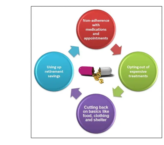
Compared to this excellent result in clinical terms, the problem of the increasing economic impact due to the high costs of targeted and immunotherapeutic drugs has raised in order to guarantee the access to patient care and the economic sustainability of the health system. In this regard, in 2013, Amy Abernethy created the term "Financial Toxicity" referred to the problem related to the cost of new therapies that can significantly influence the patient's financial balance, causing a reduction of both quality of life and access to care due to economic reasons (Figure 4) [8].

This increase in the oncological expenses is not only related to the introduction of new drugs but also due to the absence of an agreement between pharmaceutical companies and the Government concerning price stabilization, causing an increase in private insurance policies of 170% from 1999 to 2011 [9]. The difficulties in reaching an agreement not only

9

lead to an increase of insurance policies but also can cause delays in the approval and clinical applicability of emerging drugs, with direct and indirect consequences on patients’ Quality of Life.

Figure 4. Financial toxicity and its impact on patients’ Quality of Life

1.2 Aim and Structure

The aim of this study is the cost assessment in the field of oncology through the adoption of complex models, such as cluster analysis and artificial neural network, for the prediction of future costs in this area. This is more necessary day by day due to the rapidly changing therapeutic scenario of cancer patients, which corresponds to a crucial change in the cost of management in this field.

To achieve this goal, we performed a multistep analysis focused on the clinical and financial toxicity of new generation oncology drugs in order to evaluate the sustainability

10 of the health system in future years.

To assess the cost-effectiveness and predict the economic future tumor burden, we structured our study in four different sections:

 In the first section we studied the existence or not of a relationship between the costs of new generation cancer drugs and their relative toxicity through the application of a Voronoi model.

 The second section concerns the creation of a model to predict the number of new cases of cancer patients up to 2050 in the United States through the use of an artificial neural network algorithm (ANN). This step results absolutely fundamental in order to foresee the future expense associated with novel agents in different tumor types.

 The third section concerns the analysis of the costs of breast cancer, the most common tumor type among women, In particular, we compared the costs associated with the use of new targeted agents for the treatment of the two main types of breast cancer (HER2-positive and negative) in the United States with a forecast of costs up to 2035.

 The fourth section concerns the comparison of the costs of immunotherapeutic drugs (pembrolizumab and nivolumab) used in three of the most developed types of cancer, namely melanoma, lung cancer and kidney cancer by a cost-effectiveness analysis and a prediction of the expense related to the use of immunotherapy in cancer patients.

11 CHAPTER 2

USE OF VORONOI MODEL TO EVALUATE THE CORRELATION BETWEEN

2.1 Cluster analysis and health economic evaluation

In the oncological therapeutic scenario of the last two decades, new targeted drugs have been introduced, being characterized by recognizing particular molecular targets of tumor disease. Precisely for this aspect, they generally have a lower toxicity compared to traditional chemotherapeutic drugs, thus becoming a standard of care in clinical practice for the majority of tumor types. Alongside this benefit, however, the introduction of targeted drugs has greatly increased international cancer spending [10] augmenting the pharmaceutical costs by 43% in the last ten years [11].

Although new generation therapies are generally better tolerated, their toxicity can not be considered negligible. Indeed, the list of related serious adverse events includes cardiovascular, respiratory and neurological adverse events that may vary among different molecularly targeted drugs. The main challenge of researchers will be to minimize the degree of toxicity related to the use of cancer drugs to improve patients’ quality of life. This fundamental element from a medical point of view is also very important from an economic point of view. In fact, by reducing the toxicity and improving the quality of life of cancer patients, the costs related to the medical interventions necessary to manage toxicity and increase the patient's economic productivity, for example by reducing the days of absence from work, will also decrease. [12-16].

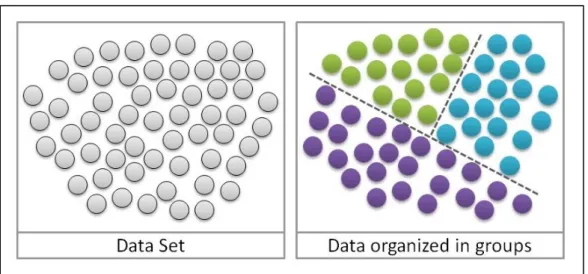
In this section, a cluster analysis has been carried out on the costs of targeted drugs and their relative toxicity profile to evaluate a possible correlation between these two variables.

12

This type of study is a set of multivariate analyzes of data whose purpose is to divide the elements into a set of data based on the similarity among them [Figure 5] [17].

Figure 5. Data distributed in cluster

Clustering is one of the techniques used in evaluating the cost-effectiveness and economic sustainability of emerging drugs [18]. In this regard, Perrier et al. in 2014 compared the costs of oncology in Italy and France, using cluster analysis and dividing data referring to diagnosis, surgery, chemotherapy, and follow-up. In this study, the authors showed a wide heterogeneity between costs between Italian and French health care [19].

On the other hand, in 2016 Liao and his group performed a non-interventional study of more than 18,000 terminal patients with kidney cancer. The research underlined, through the identification of 4 clusters, the increasing costs associated with the presence of different pathologies in the same patient [20].

In addition to the medical field, this type of statistical analysis has been applied in different areas of scientific research given its versatility such as, for example, the epidemiological, economic or engineering fields [21,22].

In our study, we created a toxicity dataset by collecting data on serious adverse events and the rate of treatment interruption of all targeted cancer drugs that were registered through

13

the approval of phase II and III studies by the United States Food and Drug Administration. The creation of the dataset was a rather complex phase and it was possible to collect the values present in the PubMed portal and represents a basic step in the research for the analysis of clinical studies. Through the cluster analysis application we have selected groups of homogeneous data that have led to the choice of suitable variables for their comparison. For the visualization of the subgroups chosen by the cluster study we used the Voronoi diagram [23] named after Georgij Voronoj, a Russian mathematician of the second half of the 1800s [Figure 6].

This type of model divides a given metric space on the basis of different types of mathematical distances from well-defined points called centroids [23].

Figure 6. Example of a Voronoi diagram [23]

Specifically these points, considering the type of distance chosen, have the ability to collect close to them the most similar data compared to those more distant. With the application of the Voronoi diagram, we investigated the way in which the data related to the toxicity behave with respect to those related to the cost, thus succeeding in giving a useful information concerning the type of relationship existing between them. In this

14

regard, Liu and his group in 2009, using the Voronoi diagram, studied the rural subdivision of a territory demonstrating that the distance between the motorways and the rivers of some land parcels was the element that mostly influenced the distribution of settlements rural [24]. Five years later, Vaz et al, showed using the same method a significant difference between the various regions of Portugal that had different models of institutional innovations [25].

Therefore, in this chapter, we evaluated the existence or not of a correlation between the cost of targeted drugs and their relative toxicity translated in terms of adverse events related to treatment and the interruption rates of therapy due to serious side effects. This study was carried out through the creation of the dataset, description of the methodological tools used in particular an explanation of the cluster analysis used and discussion of the results obtained. A peculiar element of the work is the creation of the dataset, as it has been created through a revision of the literary and represents a novelty in the oncological studies.

2.2 Material and Methods

The search and selection of a large number of clinical trials has made possible to create the database necessary for our work. Initially, through the indications contained in the PRISMA (Preferred Reporting Items for Systematic Reviews and Meta-Analyses) statement (Figure 7) [26] we selected the appropriate studies to perform the analysis through the search for key words such as "cancer", "neoplasia" and "clinical trial" on the scientific research engine PubMed since 1990 (year of development of first studies on the efficacy of these drugs) to 2018.

The second step was constituted by the choice of phase III clinical trials. These studies, if the final data reach the endpoints in terms of effectiveness predetermined a priori result,

15

lead to the approval of the experimental drugs by government agencies such as AIFA (Italian Drug Agency [27]), FDA (U.S. Food and Drug Administration [11]) and EMA (European Medicines Agency [28]).

Figure 7. Diagram of Preferred Reporting Items for Systematic Reviews and Meta-Analyses (PRISMA) [26]

For each clinical study, we collected all the fundamental information related to its drafting (authors, year of publication, reference pages etc.) and data on the efficacy and tolerability of targeted agents. Among the reported measures, we chose the time without disease progression, indicated in the studies as “Progression-Free Survival (PFS)”, the rate of severe side effects (SAE) and the rate of interruption of treatment related to toxicity (D). The currency chosen for the study analysis was the US dollar.

Regarding the clustering of data and the Voronoi diagram, we used the R 3.5.1 software for Windows (62 megabytes, 32/64 bits).

The key data for our study were those related to the toxicity of drugs, considering as important variables the SAE and D rates, included together in the Toxicity Index (TI) and their relative cost.

16

In our analysis, we have chosen five centroids that most characterize the most significant groups by combining SAE and D rates such as:

𝜙₁ = (10; 5); 𝜙₂ = (30; 15); 𝜙₃ = (45; 10); 𝜙₄ = (60; 20); 𝜙₅ = (75; 25)

The SAE rate is represented by the first value of each centroid, while the second value indicates the D rate. Specifically, the five centroids have been chosen on the basis of the different levels of SAE and D that lead to different levels of toxicity (TI): low (𝜙₁), medium-low (𝜙₂), intermediate (𝜙₃), medium-high (𝜙₄), high (𝜙₅).

The cluster 𝜙ℎ is defined by Ch, for each h = 1,2,3,4,5 and express the SAE and D rates

through the variables x and y, which are defined by the elements of the centroid (φ (h, x), φ (h, y)), for each h = 1, 2,3,4,5.

We consider the Euclidean distance, that is the original one of the Voronoi diagram, because the data groups of our analysis are characterized by the distance of the drug toxicity with the centroids. At the formal level, we can state that for each targeted agent j = 1,2,...,37 with the rate SAExj and the rate Dyj, we define:

𝑑_𝐸(𝑗, 𝜙_ℎ) = √(𝑥_𝑗− 𝜙_ℎ,𝑥)2+ (𝑦_𝑗− 𝜙_ℎ,𝑦)2

And we calculated the clusters related to targeted drugs as established by

𝐶_ℎ𝐾 _{= {𝑗 = 1, … , 37|𝑑}

𝐾(𝑗, 𝜙ℎ) < 𝑑𝐾(𝑗, 𝜙ℎ̅), ∀ℎ̅ ≠ ℎ}, ∀ 𝐾 = 𝐸, 𝑀, 𝑚, ∀ ℎ = 1,2,3,4,5.

17

the cost of one month of treatment and the costs related to each patient related to the median duration of PFS. Considering the first, we divided the data into three groups: group A (cost less than $7,000), group B (cost between $7,000 and $11,000) and group C (cost over $11,000). Regarding the cost of each treated patient for the median PFS, we have grouped the costs into 3 groups: group D with a value of less than $40,000, group E with a value between $40,000 and $80,000 and group F with a value over $80,000.

2.3 Results

At the end of PRISMA process, we have found more than 4,800 trials regarding the application of targeted agents in patients with solid tumor (Table 1) [29-65].

Target Agent

Study Characteristics Drug

Efficacy Drug Toxiciy Drug Cost

Ref Tumor Type N. of Patients Median PFS (Months) SAE (%) D Rate (%) For 1 month For median PFS

Abiraterone acetate (first

line therapy) Prostate 546 16.5 48 10 8,627 142,346 24 Abiraterone acetate

(successive line-therapy) Prostate 797 5.6 7 19 8,627 48,311 25 Afatinib NSCLC 230 11.1 49 8 6,970 77,367 26 Bevacizumab GBL 82 5.6 65.8 17.7 4,400 24,640 27 Bevacizumab RCC 327 10.2 29 28 4,400 44,880 28 Bevacizumab (first line

therapy) Colorectal 411 10.6 84,9 8.4 2,680 28,408 29 Bevacizumab (successive line-therapy) Colorectal 409 5.7 64 16 2,680 15,276 30 Cabozantinib Thyroid 219 11.2 69 16 14,300 160,160 31 Cetuximab Head &Neck 222 5.5 82 20 7,000 38,500 32 Cobimetinib+Vemurafenib Melanoma 247 9.9 62 12 26,300 260,370 33 Crizotinib NSCLC 173 7.7 33 6 11,500 88,550 34 Enzalutamide (first line

therapy) Prostate 800 8.3 28 8 7,450 61,835 35 Enzalutamide (successive

line-therapy) Prostate 872 5.7 43 6 7,450 42,465 36 Erlotinib Pancreas 282 3.8 61 10 2,450 9,310 37 Erlotinib (first line therapy) NSCLC 86 9.7 45 13 3,000 29,100 38

Erlotinib (maintainance

therapy) NSCLC 438 2.9 11 16 3,000 8,700 39 Everolimus Breast 482 7.8 23 19 7,000 54,600 40

18 Lenvatinib Thyroid 261 14.7 75.9 14.2 13,945 204,992 41 Nivolumab Squamous NSCLC 135 3.5 7 3 12,600 44,100 42 Nivolumab Non-Squamous NSCLC 292 2.3 10 5 12,600 28,980 43 Nivolumab Melanoma 210 5.1 11.7 2.4 12,600 64,260 44 Nivolumab RCC 410 4.6 19 8 6,984 32,126 45 Palbociclib (+letrozole) Breast 84 20.2 76 33 9,850 198,970 46 Palbociclib (+fulvestrant) Breast 347 9.2 69,3 2.6 9,850 90,620 47 Pembrolizumab Melanoma 277 4.1 75 6.9 23,017 94,370 48 Ramucirumab Gastric 238 2.1 57 11 13,000 27,300 49 Ramucirumab NSCLC 628 4.5 79 15 11,000 49,500 50 Ramucirumab Colorectal 536 5.7 36 11 13,000 74,100 51 Regorafenib Colorectal 505 1.9 54 44.8 7,600 14,440 52 Sonidegib BCC 79 13.1 31 22 12,000 157,200 53 Sorafenib RCC 451 5.5 34 10 6,600 36,200 54 Sunitinib RCC 375 11 7 38 7,000 77,000 55 Sunitinib GIST 207 6.4 20 9 7,000 44,800 56 T-DM1 Breast 495 9.6 15,5 5 9,800 94,080 57 Temsirolimus RCC 209 3.8 11 7 2,960 11,248 58 Trametinib+Dabrafenib Melanoma 211 9.3 32 9 16,300 151,590 59 Ziv-Aflibercept Colorectal 612 6.9 83,5 26.8 11,000 75,900 60

Table 1. Characteristics of targeted agents: Efficacy, Toxicity and Cost. The different colors in the columns related to cost refer to the different cost groups

described below in Figure 10.

BCC = Basal-cell Carcinoma; GBL = Glioblastoma; GIST = Gastrointestinal Stromal Tumor; NSCLC = Non Small Cell Lung Cancer; PFS = Progression-Free Survival;

RCC = Renal Cell Carcinoma.

Of them, 2,914 were excluded due to several reasons (i.e. phase I or in vitro studies, reviews), while 1,852 were phase II trials or studies without available data on toxicity and drug interruptions. At the and of the process, 37 studies resulted candidate to be included in this cost analysis.

The mean SAE and D rates were 44% and 14%, respectively while their mean/standard deviation were 1.68 and 1.42. Minimum and maximum SAE rate were 7% and 84.9%, while minimum and maximum D rate were 2.4% and 45%. Skewness was 0.10 for SAE and 1.48 for D rate. Kurtosis was -1.38 and 2.19, respectively.

19 targeted agents selected for this analysis.

Figure 8. Cluster analysis based on SAE and D rates

The results of the cluster analysis based on Euclidean distance are illustrated in Figure 8. These findings show clearly that five different clusters based on SAE and D rates can be identified as demonstrated by the lack of overlap between the colored areas in Figure 8. In order to represent the spatial dynamicity of the cluster analysis based on Euclidean distance we constructed a Voronoi diagram, as reported in Figure 9. This method will allow to easily collocate the future targeted agents that will be approved in next years into one of the five spatial areas only basing on their SAE and D rates.

Considering that all the drugs in each area of Voronoi diagram have resulted similar in terms of toxicity, we decided to assess if the cost of these agents is proportional to their cost. This notion results crucial to quantify the impact of oncological therapies on patients’ quality of life, which is a crucial component of the concept of “Financial Toxicity”.

20

Figure 9. Voronoi diagram based on Euclidean distance

The first step of cost analysis has been constituted by the division of drug costs into three different groups considering both the cost for one month of therapy (Figure 10A) and the cost for the entire median duration of therapy based on median PFS reported in the clinical trials (Figure 10B).

21

In the second step, we analyzed the cost of each drug in the five clusters, observing that every cluster is characterized by the presents of low, medium and high cost agents, differently distributed if we consider the cost for one month or for the entire therapy of each patient (Figure 11,12).

Figure 11. The distribution of the cost for 1 month of therapy in the five clusters:

low toxicity (cluster 1), low toxicity (cluster 2), intermediate toxicity (cluster 3), medium-high toxicity (cluster 4), medium-high toxicity (cluster 5)

Considering the cost of one month, the major percentage of low cost drugs is reported in cluster 3, while cluster 5, characterized by the maximum SAE and D rates, shows the lower rate of low cost agents (14%) and the highest rate of the most expensive drugs (58%,

Figure 11). As for the cost for median PFS cluster 4 was characterized by the major

percentage of low cost drugs (63%), while cluster 5 presented the highest rate (42%) of expensive drugs even in this setting (Figure 12).

22

Figure 12. The distribution of the cost for entire treatment of therapy in the five clusters low toxicity (cluster 1), low toxicity (cluster 2), intermediate toxicity (cluster 3),

medium-high toxicity (cluster 4), medium-high toxicity (cluster 5)

23

Through the application of the cluster analysis we observed that a three clusters based on drug cost are almost completely overlapped in both the one month (Figure 13A) and PFS

(Figure 13B) cost analysis.

2.4 Result Interpretation

In our paper, to assess the relationship between the toxicity and cost of all the oncological targeted agents approve by FDA, we considered the results coming from both the cluster analyses based on the Euclidean distance and the Voronoi Tessellation model. Our findings clearly demonstrated the lack of a relationship between the variables related to drug toxicity and the cost.

The evidence that the majority of high cost agents belong to cluster 5 (high toxicity) underlines that the price evaluation is completely independent from assessing the impact on patients quality of life. The consequences of the lack of this relationship are even more dramatic if we consider that agents with a high rate of SAE (cluster 5) are not only the most expensive but also require additional costs for the management of adverse events. At this regard, Roncato and his group [66] have tried to quantify the cost of this management. In particular, they investigated the economic amount of the adverse events associated with irinotecan, a chemotherapeutic agent commonly used in patients with colorectal or pancreatic cancer and glioblastoma. They estimated that, for each patients, over 4,800 € are required to treat the adverse event.

In the same view, Arondekar et al. [67] reported by using multivariate generalized linear models with a log-link function and gamma distribution a cost of $9,000 for the management of metabolic adverse events, $8,450 for hematologic toxicity, $6,476 for cardiovascular and $6,638 for gastrointestinal adverse events for each patients affected by metastatic melanoma. Furthermore, Bilir and his colleagues [68] classified the cost for the

24

treatment of SAE in patients with advanced melanoma, estimating that the most expensive management is associated with myocardial infarction, sepsis and coma (from $31,000 to $47,000). In their study, they also estimated a mean amount for hospitalization related to adverse events ranging from $19,000 to about $26,000) [68].

Among the limitation presented by our study, the major bias is related to the nature of this analysis, based on data of clinical studies and not from individual patients. In addition every study focused on drug toxicity may be affected by a variety of factors, including patients’ comorbidities or interactions with concomitant treatments. Moreover, patients who result eligible for clinical trials represent only a selection characterized by usually normal organ function, thus probably underestimating the real rate of adverse events in daily clinical practice. Finally, we are aware that the various adverse events differently influence patients’ quality of life, with absolutely distinct clinical, social and economic consequences.

Beyond these limitations, our study based on the construction of a dataset on toxicity and economic data on targeted agents shows the absence of a regular path, suggesting the need for a more strict connection between drug costs and their impact on patients’ quality of life.

25

CHAPTER 3

CREATION OF AN ARTIFICIAL NEURAL NETWORK TO PREDICT

3.1 Predictions of future tumor burden

In the United States, cancer is still considered the second leading cause of death (Figure

14) [69], with around 1,600 victims every day and an estimated total of over 600,000 in

2018 [70].

Figure 14. Leading causes of death in the United States (2011-2012) [69]

Despite this, over the past 25 years, there has been a real improvement of the mortality rates in cancer patients. In fact, since 1991, mortality has fallen by 25% in relation to the four most common cancers, including breast, colorectal, lung and prostate tumors [71]. In fact, as studied by de Santis and his group in their paper published in 2014, in the

26

coming years there will be more and more patients who will survive from cancer, estimated at about 18 million survivors in 2020 [72] (Figure 15).

Figure 15. Increasing rate of cancer survivors in the United States [72]

This success is related to several factors in the oncological field, such as scientific research and health choices that have had a direct effect on patients' lives and on the choice of the best available treatments. Specifically, the elements that are reducing the mortality rate include all the awareness and prevention campaigns aimed to reduce the incidence of cancer (i.e. the campaign against smoking and obesity). Moreover, research and development of new effective diagnostic techniques and the introduction of new molecular and immunotherapeutic drugs have also played a crucial role in this setting. On this scenario, a very important element for a more efficient distribution of the available economic resources and for a more detailed planning of the costs necessary for treatment, is represented by the prediction of cancer incidence rates.

27

Important elements that most influence the increase in health costs are represented both by the introduction of high expensive treatments and by the increasing demographic trend and life duration, considering that the incidence of cancer diseases are related to the age of patients [73].

The future estimate of new cases of tumors can be made by referring to different forecasting techniques. For example, the most common models in this field are the classical models based on available national registers [74-78], the Poisson linear regression model that uses contingent tables to model data [79,80] and the Bayesian age-period-cohort models [81]. Although analytical techniques are widely used to make predictions, they nevertheless have limitations that have led researchers to investigate new models of more precise future predictions.

3.2 Artificial Neural Network algorithms (ANN)

In this work, we decided to use an Artificial Neural Network (ANN) algorithm that allowed us to investigate the links between input and output variables to create predictions of future tumor incidences. This analytic technique takes into account neural networks, which are models based on the mechanisms used by the human brain for problem solving and are able to extract important information from raw data.

The first real contribution to the birth of neural networks was in 1943 when the neurophysiologist Warren Sturgis McCulloch and the mathematician Walter Pitts tried to create a first artificial neuron called "linear combinator of threshold" in their publication "A logical calculus of the ideas immanent in nervous activity". The creation of the network, in this model, was given by the combination of an appropriate number of data that were able to create simple Boolean functions, i.e. binary mathematical functions with two values (0 and 1) [82]. A new attempt was made in 1949, when the Canadian

28

psychologist Donald Olding Hebb tried to explain the complex mechanisms of the brain. It is thanks to his intuitions that "the Hebbian learning" was created, an algorithm based on the weight of the connections, that is the fact that the simultaneous activation of two neurons entails their strengthening. [83].

But the real definition of the first neural network model is found in 1958 when the psychologist Frank Rosenblatt designed the network called "Perceptron" composed of input and output variables, interconnected through an algorithm for minimizing errors (error back-propagation). Specifically, this mathematical formula modifies the weights of the connections (called synapses) based on the input and output values, creating a variation between the actual input and desired output [84].

29

During this period, up until the 1970s, the first programming languages related to artificial intelligence were introduced. The real step forward is in the 80s with the introduction of new and powerful processors on the market that have been able to run more intensive applications for analysis and simulations. From those years to today the process of technological advancement has grown so much new software programs able to really simulate the functioning of the human brain are continuously developed.

David Rumelhart (1986) defined the third layer of neural networks called the Hidden layer (H) that serves to identify learning patterns for multi-layer perceptron networks. The scholar introduced the error backpropagation that varies the weights of the edges between the nodes, bringing the real response closer to the desired one more and more.

The ANN is not an algorithm but rather a framework for parallel learning algorithms that cooperate to analyze and process complex data inputs [85]. An ANN is structured by a series of connected units called “nodes” or “artificial neurons”, with each connection, called “edge”, that can be activated according to the input and transmit a signal from a node to another. In this way, the information can be processed and transmitted by other connections (Figure 16).

In particular, each connection can transfer the output of a node i to the input of a node j [86]. The constant wi is the weight of input node i.

Mathematically, an ANN is composed by a series of functions gi(x) that can be further

divided into different functions dependent on each other (Figure 16B). A commonly used form of composition is the non linear weighted sum:

where K (tansig) is defined as the activating function (i.e. hyperbolic tangent or sigmoid function). K refers to a vector of functions gi, say:

30

g = ( g

, g

, … … , g

)

The model arising from this series of edges can analyze the short-term or long-term behavior of single neurons or networks, leading to the two main activities of ANNs: “learning” and “memory”. Learning constitutes the main function of ANN and has attracted great attention to this method. Learning is based on the ability to perform tasks by considering examples, generally with a programming not based on task-specific rules. Starting from a specific task, “learning” means to find among the set of observations the function f*∈ F, where F represents the class of functions, that optimally solve the task. Specifically, the optimal solution have to minimize the cost (C) according to the function:

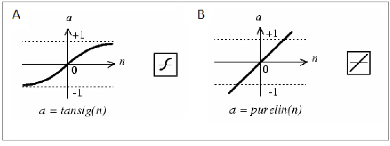
To the nodes of our ANN we have associated two activation functions: “tansing” and “purelin”. The first one in the Matlab language corresponds to the function of hyperbolic tangent "tanh(X)".

In Matlab the function “tansing” is not implemented as tanh(N) but as:

K(X) = tansig(X) = 2/(1+exp(-2*X))-1

in order to calculate the results in a faster way.

The function “purelin” corresponds to the linear function Y=X (Figure 17), which transforms the output in a set of quantities spanning in desired ranges.

31

Figure 17. Tan-Sigmoid Transfer Function (A) Linear Transfer Function

Otherwise, Matlab uses the function “TrainBR” as the training function.

Due to its flexibility of training, these types of modeling algorithms are used in different fields, including Health care, Finance and Economy [87-90]. The application of ANNs includes a series of functions:

1) System control (i.e. trajectory prediction, management of natural resources) 2) Structure or sequence identification (face, object or text recognition, radars) 3) Decision making (i.e. chess, poker)

4) Automated trading systems (i.e. Finance)

5) Filtering activity (i.e. Social Networks and e-mail spam)

Specifically, in this work, we made a prediction of the amount of new cancer cases for the most widespread neoplasms, such as prostate, breast, colon and lung cancers, through the study and development of an ANN algorithm aimed to predict the future incidence of these tumors in the United States until 2050.

3.3 Materials and Methods

3.3.1 Construction of the data sets

32

from Gapminder [91]. On the other hand, data on number of new cancer cases in the United States from 1975 to 2013 were extracted from the online public archives of National Cancer Institute [92]. As for risk factors, data on tobacco consumption were extracted from the paper published by Ng et al. [93], taking into account that the best fitting polynomial for predicting and interpolating missing data (X = year and Y = tobacco consumption) was Y = -0.3737 * X^2 – 3.7956 * X + 2363. Otherwise, the incidence of obesity were obtained from the data published by Wang et al. [94].

3.3.2 Implementation of ANNs

For each tumor type, we constructed an ANN based on the main risk factors internationally recognized. For the prediction of the future incidence of prostate cancer in the United States, we included in our ANN algorithm the three main risk factors identified by the WHO: (1) the demographic trend, (2) the life expectancy data and (3) race/ethnicity [95−97]. Due to the absence of historical series dedicated the family history of prostate cancer in the United States, we decided to not consider this as a risk factor for our analysis. We trained our ANN by using data from 1992 to 2013 on the number of new cancer cases to predict the incidence till 2050.

Breast cancer incidence grows with age [98], reaching a risk of developing this tumor in 11% of females older than 85 years [98]. In the same view, obesity correlates with an augmented risk of breast cancer [99,100] and has been associated with a worse survival in all breast tumor subtypes. In order to optimize the prediction of breast cancer new cases in the United States, we constructed an ANN based on the three risk major risk factors associated, according to WHO, to the development of this tumor: (1) the demographic trend, (2) the life expectancy and (3) the incidence of obesity. Data from 1992 to 2013 were employed for the training phase and allowed the prediction of new prostate cancer

33

cases till 2050. Concerning prostate cancer, we took into account the total population as an input variable.

Colorectal cancer can be classified as an age-dependent disease due to the notion that over 90% of these tumors occur in patients older than 50 years [101]. It has been reported that over 29% of colorectal tumors can be correlated to a Body Mass Index (BMI)>22.5 [102], with significant differences related to gender [103]. For the prediction of the incidence of colorectal cancer in the United States, we considered three main input variables in the ANN algorithm: (1) the demographic trend, (2) the life expectancy data and (3) obesity. As for prostate cancer, we used data from 1975 to 2013 for the training phase in order to validate and predict data from 2014 to 2050.

Tobacco consumption represents, as well known, the leading cause of the majority of lung cancer cases [104]. Based on the variety of pulmonary carcinogens (i.e. ionizing radiation, radon gas, etc), age can be considered as an indirect measure of exposure in both smokers and never-smokers patients [105]. In fact, several studies have evidenced the correlation between age and lung cancer incidence in non-smokers [106-108]. For the prediction of the number of new cases of lung cancer in the United States, we constructed our ANN including three input variables: (1) the demographic trend, (2) the life expectancy data and (3) the rate of tobacco consumption. The training phase was based on data from 1975 to 2013 and lung cancer incidence was predicted till 2050.

We choose as a forecasting model a layered feed forward network named “multilayered perceptrons (MLP)”, which are trained by back propagation algorithm that can adjust the connection strength between adjacent nodes. In particular, a perceptron presents distinct inputs and one output connected by a nonlinear function. This method is generally easy to use but requires a large amount of data for the thaining phase. The structure of our algorithm is illustrated in Figure 18.

34

The Learning Rate (LR) and Learning Momentum (LM) have been calculated by many trials based on the trial-and-error method. The performance of each typology was investigated by the Mean Square Error. We tried to improve the quality of our results by choosing the minimum number of nodes in order to avoid the memorization of data by the ANN and optimize their learning for generalization. The structure of our ANNs was based on three layers that have as many neurons as input variables, while the output layer has one neuron. The ANNs for colorectal, lung, breast and prostate tumors are constituted by 10, 25, 20 and 20 neurons, respectively, to implement the “tansig” function in the hidden layer.

Figure 18. The structure of our artificial neural network algorithm (ANN)

Our analysis was performed by using the Software package Matlab R2014b (Mathworks Inc.). Inputs were classified by “mapminmax” function of Matlab, to be inserted between -1 and +-1 for accounting the differences and degrees of magnitude of these variables. Taken together, about 70% of data for used to train our model and 30% to validate our predictions.

35 3.4 Results

3.4.1 Prostate cancer

The incidence of this tumor has decreased from 200cases/100,000 habitants observed in the 1990s in the United States to less than 150/100,000 in 2010. Based on our predictions, the incidence will go down till 50/100,000 from 2025 (Figure 19A).

Figure 19. Trend and predicted new cases of prostate cancer overall (A) and by Ethnicity (B=White; C=Black; D=Hispanic; E=Asian/Pacific Islander;

F=American Indian/Alaska Native)

Based on the evidence that the output also depends on races, we retrained this ANN with prostate cancer cases of White, Black, Hispanic, Asian/Pacific Islander and American

36

Indian/Alaska Native ethnicities. Regarding all the different races, our predictions show a fast decrease starting from 2010 to 2018, becoming slower from 2020 till the plateau obtained in 2050 (Figure 19A). The trend reported in the overall population is similar to that observed in White patients, which shows an incidence of less than 200/100,000 cases in the 1990s, further decreasing under 50/100,000 in 2020s (Figure 19B). The incidence is higher in Black patients (Figure 19C), who register an incidence lower that 200/100,000 only since 2012 and will fall down under 50/100,000 only after 2020 (Figure 19C). On the other hand, Asian/Pacific and American Indian/Alaska native patients are associated with a lower incidence (Figure 19E, 19F), with only American Indian/Alaska Native Races showing a decreasing trend almost steady (Figure 19F).

The fading in prostate cancer reduction from 2018 could be a consequence of the fading in life expectancy and population increase. The racial differences are related to behavioral distinctions and unequal access to high-quality health systems, although this difference is quickly diminishing.

3.4.2 Breast cancer

The incidence of this tumor can be considered almost constant in the last 25 years, considering that from 1990s has gone from 133 cases/100,000 to 124/100,000 habitants in 2015 (Figure 20).

According to our predictions, the incidence of breast cancer will fall to 123/100,000 in 2020, with a plateau in 2030 (Figure 20). Performance of Train and Validation phases showed that the ANN algorithm gained worst results (Performance of Train = 0.641; Validation phases = 0.577) in comparison with prostate, colorectal and lung cancer, may be due to the huge variety of cancer-related risk factors associated with the development of breast cancer.

37

Figure 20. Trend and predicted new cases of breast cancer. Our calculations are based on population, life expectancy and obesity data for female

3.4.3 Colorectal cancer

The incidence of this tumor has progressively augmented from 1970s (60 cases/100,000 habitants), reaching a maximum in 1985 (66/100,000, Figure 21A). Since late 1980s, the decreasing trend led to an incidence of 55/100,000 in 2000 and to 35/100,000 in 2015 (Figure 21A). According to our predictions, the incidence will account for a minimum of 30/100,000 in 2025, reaching a plateau till 2050 (Figure 21A).

Based on the role of gender in this tumor [109], we successively predicted the incidence in men (Figure 21B) and women (Figure 21C). We observed that the incidence reached its maximum in both males (79/100,000) and females (57/100,000) in 1985 (Figure 21B,

20C). Notably, our predictions show that the decrease of the incidence will reach a plateau

in 2030 in men (30/100,000), whilst the incidence will drop under 20/100,000 in 2050 in women (Figure 21B, 21C).

38

Figure 21. Trend and predicted new cases of colon cancer overall (A) and by gender (B=males; C=females). Our calculations are based on population, life expectancy and obesity

for males and females

3.4.4 Lung cancer

Since 1970s, the incidence of lung cancer has augmented from 53 cases/100,000 habitants, to a maximum of 69/100,000 in 1992 (Figure 22A). After this year, the gradually reduction in tobacco consumption has caused a decrease in the incidence of lung cancer, as evidenced in Figure 22A.

39

Figure 22. Trend and predicted new cases of lung cancer overall (A) and by gender (B=males; C=females).

This positive trend, according to our predictions, will lead to a reduction till 42/100.000 in 2030 and till 32/100,000 in 2050 (Figure 22A).

After this step, we decided to focus on the different incidence of lung cancer registered in males (Figure 22B) and females (Figure 22C), mainly due to the distinct time changes in the smoking attitude in the last 40 years.

While the maximum incidence was observed in 1984 in men (102/100,000), the highest value (54/100,000) in women was registered in 2005,may be related to the fast augment of tobacco consumption among females about 20 years later than men (Figure 22B, 22C). Of

40

note, the fall of the incidence seems to be slower in males than in females, with a plateau from 2050 (25/100,000), differently from the plateau predicted for females from 2035 (28/100,000, Figure 22B, 22C).

3.5 Result Interpretation

The variety of factors that influence the risk of developing cancer has led to the necessity of developing novel predicting tools with the ability of training from historical series of data. On this scenario, ANNs seem to represent the best candidate due to the possibility of continuously implementing the accuracy of this model by increasing the series of included input variables. Moreover, ANNs take into account the time changes of included variables, which represent a typical feature of cancer-related risk factors, such as smoking attitude, obesity or racial migrations, and can be an indirect tool to measure the impact of prevention campaigns, screening programs and innovation technologies.

Among the four tumors with the highest incidence, we observed a general decrease of tumor burden in the United States. The incidence trend of prostate cancer registered in the 1980s and early 1990s (Figure 19A) were probably associated with the introduction of prostate-specific antigen (PSA) screening, which allowed the detection of asymptomatic diseases [110]. The reduction in tumor incidence from 2010 to 2013 can be correlated with the limitations in PSA testing. Indeed, the US Preventive Services Task Force (USPSTF) published a recommendation on the use of PSA as a screening tool for prostate cancer. The task force, basing on data from Prostate, Lung, Colorectal and Ovary cancer screening study (PLCO) and the European Randomized Study of Screening for Prostate Cancer (ERSPC) trial, recommended that the potential harms of testing (erectile dysfunction, incontinence and serious surgical complications) were major than the benefits (PSA screening reduced cancer-related mortality by 4 men for every 1000 men, after 14 years of

41 follow-up) [111].

In breast cancer, the ANN did not reach good performances. The low data variability since 1990 till 2050, together with the huge series of risk factors associated with the development of this disease, ,can partially give a reason to the worst performance of our algorithm in this disease. This evidence indicates that the number of new cases does not parallel with the trends observed for age and obesity in the United States (i.e. the peak from 1995 to 2002 in cancer incidence in a time-interval characterized by the reduction of both risk factors) and support the need for identifying more effective input variables beyond the risk factors recognized by the WHO.

Regarding colorectal cancer, the reduction of the incidence rates before 2000 should be correlated with the changes in risk factors and the diffusion of screening (fecal occult blood testing (FOBT) and endoscopy) [112]. The prevalence results distinct between males and females due to a series of variables including estrogen exposure, menopausal status, insulin resistance, chronic inflammation and steroid hormones [113, 114].

As for lung cancer, it is the leading cause of cancer-related death in both men and women [115]. Decreasing its incidence constitutes a major objective for cancer researchers worldwide, and both the results of these enforces and the global prevention campaigns aimed to reduce smoking attitude are represented in Figure 22A, which show a drop in the incidence of lung cancer. This progressive decrease would be even faster as an effect of the global policy towards the 2040 tobacco-free world goal [116]. Concerning the gender differences (Figure 22B, 22C), they parallel with the historical attitudes in tobacco consumption, with females starting to smoke in large number later and at older ages than men.

However, our study has a series of limitations, including: (1) biases related to data selection, although partially decreased by performance analysis and validation phase; (2)

42

the variety of cancer-associated risk factors, which may be only partially represented by the three major risk factors reported by WHO for the four most frequent tumours.

In conclusion, our model based on ANN algorithm to predict tumor burden in US could represent a crucial resource to plan and evaluate cancer-control programs. Urgent worldwide policies towards a dramatic decrease of cancer-related risk factors are absolutely needed and will contribute to the drop of incidences and the route to cancer eradication in future decades.

43

CHAPTER 4

ESTIMATION OF PRESENT AND FUTURE COSTS OF BREAST CANCER

4.1 Therapeutic and socio-economic landscape of breast cancer

Breast cancer is the most common cancer among women in the world and is the leading cause of death in developing countries with an estimated increase of 6 million new cases in the next 20 years [117]. It has been estimated that 266,120 new cases of invasive breast cancer and 63,960 of non-invasive tumors in 2018 in the United States [118] (Figure 23).

Figure 23. Annual breast cancer incidence rate per 100,000 people [118]

In Italy, the Italian Association of Tumor Registry (AIRTUM) together with the Italian Association of Medical Oncology (AIOM) estimated in 2018 52,800 new cases of breast cancer, with an increase of about 8,000 new cases compared to 2011 [119].

In 2017, Stefano Capri and his group, using the data from the cancer register of the Agency of Health Protection of the Province of Milan, estimated how the costs of cancer are distributed in the different stages of the disease with the aim of evaluating the variables

44

that influence the average cost of treatment of breast cancer. Through a generalized linear model they studied the costs related to 12,580 cases of breast cancer with a total cost of € 22,515 per patient inclusive of average costs for diagnosis, treatment, follow-up and for medical dedicated to the treatment of patients [120] (Figure 24).

Figure 24. Distribution of costs related to the volume of hospital in Italy [120]

An important element in breast cancer treatment has been the introduction, even in this type of disease, of "molecular target" drugs, which are directed towards specific targets expressed in cancer cells, increasing patients’ life expectancy. Alongside this success, however, these new drugs have a much higher cost than previous agents. This can be explained by the higher costs related to the research and development of these drugs, leading to both an increase of the investment in the development of new drugs from $10,000 (1960) to $70,000 (2010) and a reduction of the death rate from 1,300/100,000 to 800/100.000 patients [121].

45

In recent years, the study and research of molecular targets associated with a better prognosis for cancer patients and fewer side effects of therapies is becoming more and more important. Specifically, it was discovered that a part of breast tumors express the oncogene called HER2. This allowed to identify two well-defined disease classes, HER2-positive and HER2-negative tumors. The progress in understanding the role of presents of HER2 has allowed, in this type of disease, to develop drugs such as Trastuzumab, Pertuzumab and Lapatinib that are targeted towards this genetic alteration. In contrast, in the HER2 negative patients, drugs such as Bevacizumab, Everolimus and Palbociclib have been developed, leading to an advantage in terms of overall survival and quality of life. The purpose of the following work is to identify and estimate the different costs of the use of these drugs by making a prediction on the costs incurred for their employment.

4.2 Materials and Methods

We estimated a cost for each patient basing on an ideal height 1.60 m and an ideal weight of 60 kg and considering every patient as a candidate to receive all the drugs approved for the specific type of breast cancer (for HER2 positive: Pertuzumab + Trastuzumab, T-DM1 and Lapatinib; for HER2 negative: Bevacizumab, Everolimus and Palbociclib). The doses of Lapatinib, Everolimus and Palbociclib are fixed and orally administered for all patients, independently from their height and weight. The dose of Bevacizumab is calculated considering 5 mg of drug for each kg of patient weight. As for Pertuzumab plus Trastuzumab and T-DM1, the doses are calculated based on the body surface obtained by Mosteller formule:

46

To estimate the cost of the entire treatment for each patient, we considered the median duration of treatment expressed in the clinical trials as Progression-Free Survival (PFS), defined as the time from the start of targeted therapy to tumor progression or death.

We used to estimate the total number of patients treated in the United States from 2015 to 2050 the results obtained by ANN reported in Chapter 3. To quantify the number of patients who will receive a treatment through targeted approaches, we have to consider that only the 20% of the total number of patients with a diagnosis of breast cancer will develop metastases during their life [122]. Of them, 20% will result affected by breast cancer tumors harboring HER-2 positivity, while the 80% will be affected by HER2 negative tumors [123].

4.3 Results

4.3.1 Estimated per patient cost with HER2 positive tumours

As previously reported, patients affected by HER2 positive breast tumors can receive three different target therapies: (1) the combination of Pertuzumab and Trastuzumab, (2) T-DM1 and (3) Lapatinib. The first combination is characterized by a median duration of treatment of 18.5 months in the 808 patient enrolled in the clinical trial [124]. Otherwise, the administration of T-DM1 was associated with a median disease control of 9.6 months in the clinical trial that has led to its approval by FDA [125], while Lapatinib registered a median PFS of 8.4 months [126].

Taking into account the ideal height and weight reported in the Materials and Methods, we calculated the cost for one month of therapy and for the median duration of treatment expressed by median PFS for each agent. The highest cost is registered by the combination of Pertuzumab and Trastuzumab. Indeed, the monthly cost of this therapeutic approach can be estimated in $9,390 ($4,890 + $4,500), with a cost for the median entire treatment

47 of $173,715 (Figure 25).

Figure 25. Estimated per patient cost with different drugs ($)

On the other hand, the costs for the median duration of target therapy with T-DM1 and Lapatinib result lower and can be estimated in $94,080 and $24,360, respectively (Figure

25).

4.3.2 Estimated per patient cost with HER2 negative tumours

As previously in the Materials and Methods, patients affected by HER2 negative tumors can receive three different therapeutic approaches: (1) Bevacizumab, (2) Everolimus (3) Palbociclib. The first drug registered a median duration of treatment of 11.8 months in the clinical trial that led to its approval by FDA [127]. On the other hand, treatment with Everolimus reported a median time of disease control of 6.9 months [128]. As for Palbociclib, two different studies [129,130] showed a median duration of treatment of 20.2 and 9.2 months, respectively.

48

$90,620 considering both the clinical trials focused on this agent [129,130], with an average per patient cost of $144,795 (Figure 25). On the other hand, the costs for the median duration of target therapy with Bevacizumab and Everolimus result lower and can be estimated in $31,860 and $48,300, respectively (Figure 25).

4.3.3 Estimated total cost for HER2 positive and negative tumours (2015-2050)

Firstly, we compared the per patient cost of the two subpopulations given by the addiction of the cost of each drug, which was $292,155 for HER2 positive and $224,955 for negative tumours, respectively. As for the number of metastatic patients estimated by our ANN algorithm and reported in Table 2, it is evident that the incidence will decrease till 2030 and successively slowly increase from 2035 to 2050 (Table 2).

YEAR Estimated N. of patients Pertuzumab and Trastuzumab

T-DM1 Lapatinib Bevacizumab Everolimus Palbociclib

2015 24856 863,572,008 467,690,496 121,098,432 633,529,728 960,435,840 2,879,219,616 2020 24704 858,291,072 464,830,464 120,357,888 629,655,552 954,562,560 2,861,612,544 2025 24622 855,442,146 463,287,552 119,958,384 627,565,536 951,394,080 2,852,113,992 2030 24511 851,585,673 461,198,976 119,417,592 624,736,368 947,105,040 2,839,256,196 2035 24551 852,975,393 461,951,616 119,612,472 625,755,888 948,650,640 2,843,889,636 2040 24560 853,288,080 462,120,960 119,656,320 625,985,280 948,998,400 2,844,932,160 2045 24567 853,531,281 462,252,672 119,690,424 626,163,696 949,268,880 2,845,743,012 2050 24568 853,566,024 462,271,488 119,695,296 626,189,184 949,307,520 2,845,858,848

Table 2. Estimated total cost with different drugs ($)

Starting from HER2 positive tumors, treatment with Pertuzumab and Trastuzumab is associated with the highest cost in 2015, accounting for $863,572,008, which is

49

approximately two folds and seven folds the estimated cost of treatment with T-DM1 ($467,690,496) and Lapatinib ($121,098,432), respectively (Table 2, Figure 26). Based on these results, the estimated total cost for the treatment of patients with HER2 positive breast tumours in 2015 is $1,452,360,936 (Table 3, Figure 27), with Pertuzumab and Trastuzumab representing the 59.5% of the total amount. Concerning the predictions for 2050, the total cost for patients with HER2 positive tumours is estimated at $1,435,532,808 (Table 3, Figure 27), registering a reduction of about 1% compared to 2015.

Figure 26. Estimated total cost with different agents (expressed in one hundred million $)

Regarding the expense for patients with HER2 negative breast tumours, the highest estimated cost in 2015 is associated with the use of Palbociclib ($2,879,219,616, Table 2,

Figure 28), while the lowest is registered by Bevacizumab ($633,529,728, Table 2, Figure 28).

50

YEAR Estimated N. of patients HER 2 POSITIVE HER 2 NEGATIVE

2015 24856 1,452,360,936 4,473,185,184 2020 24704 1,443,479,424 4,445,830,656 2025 24622 1,438,688,082 4,431,073,608 2030 24511 1,432,202,241 4,411,097,604 2035 24551 1,434,539,481 4,418,296164 2040 24560 1,435,065,360 4,419,915,840 2045 24567 1,435,474,377 4,421,175,588 2050 24568 1,435,532,808 4,421,355,552

Table 3. Estimated total year cost for HER2 positive and HER2 negative breast tumors ($)

The total cost for HER2 negative tumours in 2015 is estimated in $4,473,185,184, with Palbociclib, Everolimus and Bevacizumab accounting for the 64.4%, 21.5% and 14.1%, respectively (Table 3, Figure 27).

Figure 27. Estimated total year cost for HER2 positive and HER2 negative breast tumors (expressed in one hundred million $)

51

As for HER2 positive tumours, we estimate that the total cost will decrease by about 1% in 2050 (Table 3, Figure 27).

Figure 28. Estimated total cost with different agents (expressed in one hundred million $)

Taken together, these data show that the cost for the HER2-negative patients was $3,0208,24,248 higher that for HER2-positive tumors in 2015, and this difference will decrease to $2,985,822,744 in 2050 (Table 3, Figure 27).

4.3 Result Interpretation

In recent years the therapeutic scenario in the field of cancer is completely changing. In particular, therapeutic treatments for breast cancer are evolving towards specific therapies no longer generalized, for example through the use of targeted drugs. In our study, we estimated the increasing costs of breast cancer treatment in the United States. This is mainly due to the entry into clinical practice of combinations of drugs such as Pertuzumab and Trastuzumab together with Palbociblib for the treatment of HER2 positive and