PAPER • OPEN ACCESS
Efficiency of quantum controlled non-Markovian
thermalization
To cite this article: V Mukherjee et al 2015 New J. Phys. 17 063031
View the article online for updates and enhancements.
Related content
Quantum non-Markovianity: characterization, quantification and detectionÁngel Rivas, Susana F Huelga and Martin B Plenio
-Foundations and measures of quantum non-Markovianity
Heinz-Peter Breuer
-Simulation of indivisible qubit channels in collision models
Tomáš Rybár, Sergey N Filippov, Mário Ziman et al.
-Recent citations
Time-optimal control of the purification of a qubit in contact with a structured environment
J. Fischer et al
-Experimental emulation of quantum non-Markovian dynamics and coherence protection in the presence of information backflow
Deepak Khurana et al
-Quantum speed limits: from Heisenberg’s uncertainty principle to optimal quantum control
Sebastian Deffner and Steve Campbell
PAPER
Efficiency of quantum controlled non-Markovian thermalization
V Mukherjee1,2, V Giovannetti1, R Fazio1,3, S F Huelga4, T Calarco2and S Montangero21 NEST, Scuola Normale Superiore & Istituto Nanoscienze-CNR, I-56126 Pisa, Italy 2 Institute for Complex Quantum Systems & IQST, Universität Ulm, D-89069 Ulm, Germany 3 Centre for Quantum Technologies, National University of Singapore, 117543, Singapore 4 Institut für Theoretische Physik & IQST, Universität Ulm, D-89069 Ulm, Germany
E-mail:[email protected]
Keywords: optimal control of quantum systems, open quantum systems, non-Markovian dynamics, quantum speed limit
Abstract
We study optimal control strategies to optimize the relaxation rate towards the
fixed point of a
quantum system in the presence of a non-Markovian (NM) dissipative bath. Contrary to naive
expectations that suggest that memory effects might be exploited to improve optimal control
effectiveness, NM effects influence the optimal strategy in a non trivial way: we present a necessary
condition to be satisfied so that the effectiveness of optimal control is enhanced by NM subject to
suitable unitary controls. For illustration, we specialize our
findings for the case of the dynamics of
single qubit amplitude damping channels. The optimal control strategy presented here can be used to
implement optimal cooling processes in quantum technologies and may have implications in
quantum thermodynamics when assessing the efficiency of thermal micro-machines.
1. Introduction
Controlling quantum systems by using time-dependentfields [1] is of primary importance in different branches of science, ranging from chemical reactions [2,3], NMR [4], molecular physics [5] to the emergent quantum technologies [6–8]. Investigations on optimal control of open quantum systems mostly focus on memoryless environments [9–11] and specifically on those situations where the reduced dynamics can be described by a
Markovian master equation of the Lindblad form [12]. In this context, optimal control applications to open quantum systems have been explored in different settings [5,13–18] and recently the ultimate limits to optimal control dictated by quantum mechanics in closed and open systems [19–22] and the complexity of dealing with many-body systems [23–25] have been determined. Time-optimal quantum control has been extensively discussed for one qubit systems in a dissipative environment [9,26] and the optimal relaxation times determined in [27]. These studies might have both fundamental and practical applications, for example in assessing the ultimate efficiency of quantum thermal machines [28], or to implement fast cooling schemes which have already proven to be advantageous [29,30].
However, introducing a Markovian approximation requires some constraints on system and environment, which may not be valid in general [31,32]. Consequently, incorporating non-Markovian (NM) effects of the environment, in a sense that will be defined more precisely below, might be a necessity in a many experimental situations. Recently, the possible influence of memory effects on the orthogonality catastrophe [33], on
quantum speed of evolution [34] and on quantum control [35,36] have been analyzed. Here, we present a study of the optimal control strategies to manipulate quantum systems in the presence of NM dissipative baths and compare the performance of optimal control with the case of operating subject to a Markovian (M)
environment.
Intuitively, the absence of memory effects in the dynamics of open quantum systems is linked to the possibility of identifying well separated time scales in the evolution of system and environment. Recently, a number of proposals have been put forward to quantitatively characterize this effect in terms of explicit NM measures [37–40]. In this light, one can define an evolution to be Markovian if described by a quantum dynamical semigroup (time-homogeneous Lindbladian evolution) [41], which would be the traditional
OPEN ACCESS
RECEIVED
3 February 2015
REVISED
5 May 2015
ACCEPTED FOR PUBLICATION
26 May 2015
PUBLISHED
23 June 2015
Content from this work may be used under the terms of theCreative Commons Attribution 3.0 licence.
Any further distribution of this work must maintain attribution to the author(s) and the title of the work, journal citation and DOI.
Markovianity considered in most previous work on open system control. However, other definitions encompass this as a special case while allowing for more general, non-homogeneous generators, albeit still ensuring the divisibility of the associated dynamical map and the unidirectionality of the system–environment information flow, and therefore the absence of memory effects in the dynamics of the system [42–45]. Relevant for our analysis is the definition of Markovian evolution in terms of the divisibility of the associated dynamical map [46]. When the dynamics is parametrized using a time-local master equation, the requirement of trace and hermiticity preservation, yields a generator of the form
)
(
t H t t t t H t t t A t t A t A t A t t ˙ ( ) i ( ), ( ) ¯ ( )( ( )) i ( ), ( ) ( ) ( ) ( ) ( ) 1 2{ ( ) ( ) ( )} , (1) s s s k k k k k k † † ⎡⎣ ⎤⎦ ⎡⎣ ⎤⎦∑
ρ ρ ρ ρ γ ρ ρ = − + = − + − where¯ ( )t is a time dependent Lindblad superoperator,γk( )t are generalized (i.e. not necessarily positive) decay rates, the Ak(t)ʼs form an orthonormal basis for the operators for the system, see e.g. [47] (hereafterℏ has been set equal to one for convenience) and Hs(t) is the effective Hamiltonian acting on the system. Equation (1) generalizes the familiar Lindbladian structure to include NM effects while maintaining a time-local structure. However, apart from same special cases, it not known which are the conditions which Hs(t), Ak(t), andγk( )t have to satisfy in order to guarantee complete positivity (CP) [47–51], i.e. the fundamental prerequisite which under fairly general assumptions is needed to describe a proper quantum evolution [31,32]. In what follows we will focus on a simplified scenario where theγk( )t ʼs either are null or coincide with an assigned function tγ( ), and where the Ak(t)ʼs are explicitly time-independent. Accordingly, in the absence of any control Hamiltonian applied during the course of the evolution, we assume a dynamical evolution described by the equation
t t t
˙ ( ) ( ) ( ( )), (2)
ρ =γ ρ
where is a (time-independent) Lindblad generator characterized by having a unique fixed pointρfp(i.e. ( )ρ =0
iffρ=ρfp). For this model, in the absence of any Hamiltonian term (i.e. H ts( )=0) CP over a time interval[0,T]is guaranteed when [48]
t t t T
( )d 0, [0, ], (3)
t 0
∫
γ ′ ′ ⩾ ∀ ∈while divisibility (i.e., Markovianity) is tantamount to the positivity of the single decay rate at all times [47]: if there exists a time interval whereγ( )t becomes negative, the ensuing dynamics is no longer divisible and the evolution is NM. In this context we will assume a control Hamiltonian Hs(t) to represent time-localized infinitely strong pulses, which induce instantaneous unitary transformations at specific control times. This corresponds to writing H ts( )=
∑
jδ(t− tj)Θs( )j, whereΘs( )j are time independent operators which actimpulsively on the system at t=tj(δ( )t being the Dirac delta-function), at which instants one can neglect the
contribution from the non-unitary part, and represent the master equation byρ˙ ( )t ≈ −i⎡⎣H ts( ),ρ( )t ⎤⎦.
Therefore the resulting dynamics is described by a sequence of free evolutions induced by the noise over the intervals t∈ [ ,t tj j 1+ ]interweaved with unitary rotations Uj=exp[ i−Θs( )j], i.e.
t ( ) ( (0)), (4) j j j fin 1 1 0 in ρ ρ = ◦ ◦ ◦ ◦ ⋯ ⋯ ◦ ◦ ◦ − where j exp[ ¯ ( )]t t t j j 1
∫
= + ,( )⋯ =U( )⋯ U†and‘◦’ is the composition of super-operators. When only
two control pulses are applied (thefirstinat the very beginning and the second at the very end of thefin
temporal evolution), the non-unitary evolution is described by equation (2) and CP of the trajectory (4) is automatically guaranteed by equation (3), the scenario corresponding to the realistic case where one acts on the system with very strong control pulses at the state preparation stage and immediately before the measuring stage. When morejʼs are present, the situation however becomes more complex. There is no clear physical
prescription which one can follow to impose the associated dynamics on the system at least when the dissipative evolution is assumed to be NM. Consider for instance the casefin◦1◦1◦0◦in( (0))ρ , where1is a
non-trivial unitary. Even admitting that the latter is enforced by applying at time t1a strong instantaneous control pulse, there is absolutely no clear evidence that the open dynamics fort ⩾t1should be still described by
the same generalized Lindbladianγ( )t , the system environment being highly sensitive to whatever the system itself has experienced in its previous history.
We note that in a more realistic scenario, any control pulse will have a non-zero widthδtin time. Clearly, a sufficiently largeδtcan invalidate the assumption of applying control pulses only at the very beginning and the very end, thereby modifying the dynamics significantly as described above. However, one can expect the
2
assumption of instantaneous pulses to be valid as long asδtis negligible compared to the time scale associated with the dynamics in absence of any control.
Keeping in mind the above limitations, in this work we attempt for thefirst time a systematic study of optimal control protocols which would allow one to speed up the driving of a generic (but known) initial state
(0)
ρ toward thefixed pointρfpof the bare dissipative evolution for the model of equation (2) which explicitly includes NM effects. We arrive at the quantum speed limit times when application of only two control pulsesin
and , at initial and final times respectively, is enough to follow the optimal trajectory. On the other hand, wefin
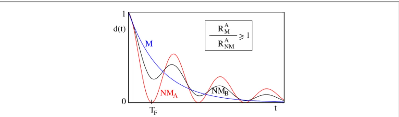
present lower bounds to the same when optimal control strategy demands unitary pulses at intermediate times as well. We show that the efficiency of optimal control protocols is not determined by the M/NM divide alone but it depends drastically on the behavior of the NM channel: if the system displays NM behavior before reaching thefixed point for the first time, NM effects might be exploited to obtain an increased optimal control efficiency as compared to the M scenario. On the contrary, NM effects are detrimental to the optimal control effectiveness if information back-flow occurs only after the system reaches the fixed point (see figure1). These results are valid irrespective of the detailed description of the system, i.e. its dimension, Hamiltonian, controlfield, or the explicit form of the dissipative bath.
2. The model
The divisibility measure for the model equation (2) is equivalent to the characterization of memory effects by means of the time evolution of the trace distance [52]. This provides an intuitive characterization of the presence of memory effects in terms of a temporary increase in the distinguishability of quantum states as a result of an information back-flow from the system and into the environment that is absent when the evolution is divisible [53]. As a result, a divisible evolution for which the single decay rateγ( )t ⩾ 0at all times will exhibit a monotonic decrease of the trace distance of any input state towards a (assumed to be unique)fixed pointρfpof the Lindblad generator [54]. On the contrary, as illustrated infigure1, the behavior of the trace distance can be non-monotonic when the dynamics is NM. In this case, there exist time interval(s) whereγ( )t becomes
negative. Denoting by d t( )= ∣∣ρ( )t −ρfp∣∣the trace distance betweenρ( )t and thefixed pointρfp, it straightforwardly follows that d t˙ ( )⩽0∀tin the M limit. Looking at this quantity one can classify NM dynamics into two distinct classes (seefigure1): thefirst one (class A) is defined by those dynamics where the system reaches thefixed point at time TFbeforeγ( )t changes sign i.e.,γ( )t ⩾ 0and d t˙ ( )⩽0for0⩽t <TF. In
this case, the NM dynamics reaches thefixed pointρfpand then start to oscillate. On the other hand, class B dynamics is characterized byγ( )t that changes sign (and correspondingly d t˙ ( )>0) at some time t<TF, that is
the solutions of the equationγ( )ts =0are such that ts< TFfor at least one s. In contrast, in the M dynamics d(t)
always decreases monotonically and asymptotically to d t( → ∞ =) 0.
NM channels of class A/B arise from different physical implementations. As an illustration, the damped Jaynes–Cummings model exemplifies a class A dynamics. Here a qubit is coupled to a single cavity mode which in turn is coupled to a reservoir consisting of harmonic oscillators in the vacuum state (see equation (6)) [31,55– 57]. On the other hand, dynamics similar to class B can arise for example in a two level system in contact with an environment made of another two level system, as realized recently in an experimental demonstration of NM dynamics [58].
Figure 1. Schematic diagram of NM dynamics in class A (red line) and class B (black line). The instantaneous trace distance
d t( )= ∣∣ρ( )t −ρfp∣∣starts increasing only after the system reaches thefixed point when∣ ∣ → ∞γt in case of class A, while it shows oscillatory behavior even before it reaches thefixed point in case of class B. In comparison dynamics for a M channel is shown by the blue line where d(t) decreases monotonically and assymptotically to d t( → ∞ =) 0. The speedup obtained by M dynamics is always bigger than that obtained for the NM one, i.e., RMARNMA ⩾1in case the NM evolution is of class A, while the Markovian limit can be surpassed by NM of class B.
As we will see hereafter, the difference between class A and B appears to drastically affect the performance of any possible optimal control strategy to improve the speed of relaxation of the system towards thefixed point.
We assume full knowledge of the initial state and we allow for an error tolerance of 0< ϵ≪1, considering that the target is reached whenever the condition d t∣ ( )∣ ⩽ϵis satisfied. To obtain a lower bound on the minimum time TQSLneeded to fulfill such constraint we restrict our analysis to the ideal limit of infinite control which allows us to carry out any unitary transformation instantaneously along the lines of (and with all the limitations associated with) the formalism detailed in equation (4). In the limit of infinite control an important role is played by the Casimir invariantsΓj(j =2, 3,…,Nfor a N level system). The Casimir invariants of a
stateρ are related to the trace invariantsTr( )ρj (j =2, 3 ,...,N) and they cannot be altered by unitary
transformation alone [10,59]. For example, a two level system has a single Casimir invariant—its purity P=Tr ( )ρ2, which remains unchanged under any unitary transformation. Consequently, any optimal strategy
with the controls restricted to unitary transformations only, would be to reach a stateρ characterired by all Casimir invariants same as those ofρfpin the minimum possible time. Following this we can apply a unitary pulse to reach thefixed point instantaneously. Clearly, any constrained control will at most be as efficient as the results we present hereafter, based on the analysis we have presented previously for the case of M
dynamics [5,27].
In what follows, we will analyse class A and B channels independently.
Class A: as shown infigure1, in the NM regime d(t) goes to zero at t=TFwhenρ= ρfpand(ρfp)= 0. At
the same time we expect∣γ( )t ∣ → ∞at t ≈TFin order to havefinite tρ˙ ( )= γ( ) ( ( ))t ρ t even for
t
( ( ))ρ ≈ (ρfp)= 0
, as is required for a non-monotonic d of the form shown infigure1. Notice thatγ( )t and hence the time t=TFat whichγ( )t → ∞are in general independent ofρ. Consequently any optimal control
protocol which involves unitary transformation ofρ( )t generated by Hs(t) at earlier times t<TFfollowed by
non-unitary relaxation toρfpis expected to be ineffective in this case and we have TQSL= TF. That is, the gain (or
efficiency) of optimal trajectory in the NM class is RNMA =T TF QSL=1. One can easily see T TF QSL =1implies
absence of any speed up, whereas any advantage one gains by optimal control can be quantified by T TF QSL>1. On the other hand in the M limitγ( )t =γ0isfinite and constant, and the system relaxes asymptotically to the fixed point in the absence of any control. In this case we introduce an error toleranceϵ ≪1, such that we say the target state is reached if d T∣ ( F)∣ ⩽ϵ. Clearly, TFincreases with decreasingϵ diverging to TF→ ∞in the limit
0
ϵ → , as can be expected forfiniteγ0. Therefore the above argument of∣γ( )t ∣ → ∞at t≈TFdoes not apply in
this case and in general one can expect the time of evolution to depend on the initial state. Consequently the quantum speed up ratio RMAcan exceedRNMA ≈1, as is explicitly derived below in the case of a two level system in
presence of an amplitude damping channel. Similar arguments apply also in the case when an additional unitary transformation is needed at the end of the evolution to reachρfp, where RMA→ ∞forϵ →0[27].
Our above result RMA⩾RNMA can be expected to be valid in a more generic scenario with
t t t
˙ ( ) ( ) ( ( ))
k k k
∑
ρ = γ ρ as well, where not allγkʼs (≠0) are same,kʼs are the time independent Lindblad
generators and the uniquefixed pointρfpis defined byk(ρfp)=0for all k. In this case at least one of theγkʼs
can be expected to diverge at time t=TFin order to ensure class A NM dynamics as shown infigure1thus
making any optimal control ineffective as detailed above. We note that one can have dynamics with time dependent Lindblad generators and uncontrollable drift Hamiltonians acting on the system during the course of the evolution, in addition to the instantaneous control pulses, as well. The drift Hamiltonians can be expected to modify the Lindblad generators thus making the problem more complex; however the analysis in this case is beyond the scope of our present work.
Class B: here we focus on systems of class B where as already mentionedγ( )t changes sign for ts<TFwith
s=1 ,...,Ns. Clearly, in this case∣γ( )t ∣does not necessarily diverge for any t. Consequently the arguments
presented above for class A fails to hold any longer and the time of relaxation to thefixed point can in general be expected to depend onρ( )t (and hence on Hs). Furthermore, it might be possible to exploit the NM effects such that even though d t˙ ( )>0for t1⩽t⩽ t2one can, by application of optimal control, make sure thatΓ˙ ( )j t >0
and maximum∀t j, (where we have assumedΓj(t= 0)<Γjf ∀jandΓjf denotes the jth Casimir invariants for
thefixed pointρfp). This presents the possibility of exploiting NM effects to achieve better control as opposed to the M dynamics, as is presented below for the case of a two level system in the presence of an amplitude damping channel. However we stress that this is not a general result and explicit examples can be constructed where this is actually not true.
2.1. Generalized amplitude damping channel
Let us now analyze in detail the generic formalism outlined above for the specific case of a two level system in contact with NM amplitude damping channels of the two classes introduced before.
We consider the non-unitary dissipative dynamics described by the time local master equation acting on a 2 × 2 reduced density matrixρ( )t of a qubit and we consider the time independent Linbladian given by
4
{
}
{
}
t t t t t t ( ( )) ( ) 1 2 , ( ) , ( ( )) ( ) 1 2 , ( ) , (5) 1 2 ⎜ ⎟ ⎜ ⎟ ⎛ ⎝ ⎞⎠ ⎛ ⎝ ⎞⎠ ρ σ ρ σ σ σ ρ ρ σ ρ σ σ σ ρ = − = − + − − + − + + − withσ±being the raising/lowering qubit operators and1 βgives the temperature of the bath. The system
evolution is given by equation (2), and we will focus on two different functional dependence of the parameter
t
( )
γ corresponding to the class A and B dynamics. We will analyze the system evolution following the Bloch vector r ⃗ representing the stateρ=(I+ ⃗r. ) 2σ⃗ inside the Bloch sphere, where the unitary part of the dynamics generated by Hsinduce rotations, thus preserving the purity P= (1+ ∣ ⃗ ∣r 2) 2. In contrast, in general the action of the noise is expected to modify the purity as well.
Class A: an example of this class of dynamics is obtained under the assumption
t
tg
g tg tg
its width in time tδ ≪1 ⎡⎣γ0(eβ +1)⎤⎦in the M limit of
0
λ≫γ, while in the NM limitλ≪γ0one has
t 1 0(e 1)
δ ≪ λγ β+ .
Class B:finally, we investigate a particular case belonging to the class B dynamics and compare it to the previous case. As in the previous case we consider a time evolution described by a master equation equation (2) with given by equation (5); however for our present purpose we formulate aγ( )t given by
t t
( ) e tcos( ) , (8)
γ = −ζ Ω
withζ Ω, being two positive constants satisfying the CP condition equation (3). With this choice, in the absence of the control Hamiltonian, NM effects manifest themselves for(2n+1)π 2<Ωt<(2n+ 3)π 2for integer
n⩾0asγ( )t changes sign atΩt= (2n+1)π 2, simultaneously altering the sign of d t˙ ( ) to d t˙ ( )> 0. With a proper choice of parameters one can makeγ( )t (and hence d(t)) exhibit oscillatory dynamics for1> d>0. As for the previous example, also in this case the extremals of v are independent ofγ( )t and determined by( ( ))ρ t
only. Therefore they occur at exactly the same points as for class A (6), i.e., atθ =0,πandarccos(r rf). In this case an instantaneous pulse would correspond to its time width tδ ≪min{1ζ, 1/ , 1/(eΩ β +1)}.
The unconstrained optimal strategies are now modified as follows. In the case of cooling, the optimal strategy is to follow the pathθ=πfor0⩽ t<TQSLcool, during which time the purity increases monotonically,
where we have assumed the system reaches the target at t=TQSLcool<π (2 )Ω for simplicity. Consequently the optimal strategy demands a single pulse at time t = 0 only to makeθ= π, which corresponds to an evolution operator of the formfin◦D◦ . Clearly, this evolution is CPT as already discussed in sectionin 1with D
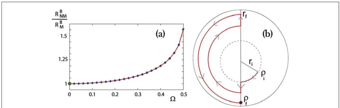
depending onγtand (see equations (5) and (8)) and is thus possible to implement physically. Infigure3(a) we report the speedup obtained by such optimal strategy for different values ofΩ in equation (8), where we have takenϵ =0.01large enough so thatΩTQSLcool< π 2. In this case we arrive at the M limit by settingΩ =0; as can be clearly seen the speed up in the NM limit is such that RNMB >R ,MB ∀Ω>0showing that there exist scenarios where NM effects can be exploited to improve the control effectiveness. On the contrary, if the system does not reach the target forΩTQSLcool<π 2, the optimal strategy changes: atΩt= π 2,γ( )t and hence v change sign, leading to decrease (increase) of purity forθ=π(θ =0). Interestingly, we can take advantage of this effect by makingθ =0at t= π (2 )Ω , where v exhibits a maximum forγ( )t < 0. As mentioned before, application of a unitary pulse during the course of an evolution may change the form ofγ( )t and (see equation (4)). However, for simplicity let us assume v changes sign at t=(2n+ 1)π 2and assumes extremum values atθ =0,πand
r r
arccos(− fp)even in presence of unitary control. One can easily extend our analysis to a more generic case where the simplifying assumptions do not hold by following the path of maximum (minimum) v for cooling (heating). Let usfirst consider the case where the system reaches the target rz=rf − ϵat t =TQSLcool<3 (2 )π Ω.
In such a scenario, as depicted infigure3(b), we let the system evolve freely forπ(2 )Ω <t⩽ TQSLcool, following which we take the system toθ= πand rz= −rf +ϵ, thus obtaining the desired goal. Clearly, an optimal path
exists in case of the class B NM channel, which if possible to be followed by application of suitable unitary controls, helps in cooling and in particular might make it possible to reach thefixed point in finite time (if
0
ϵ = ). Generalization to the caseΩTQSLcool>3π 2where multipleπ rotations are needed is straightforward. However, we emphasize that the strategy presented above forΩTQSLcool>π 2follows an evolution operator of the
Figure 2. (a) Parametric plot showing variation of timeTQSLcoolof reaching thefixed point with λ andγ0forβ = , r2 i= 0.5 andϵ =0.01.
The Markovian (M) and non-Markovian (NM) regions are separated by the blue line on theλ−γ0plane. (b) Plot showing variation of quantum speed up ratio RAwithλ and
0
γforβ = ,2 rxi=0.3, ryi=0,rzi=0.4andϵ =0.01. RAsaturates to RMA≈2(RNMA ≈1)
in the extreme M (NM) limit.
6
form equation (4) with unitary pulses applied at intermediate times. Consequently our analysis gives a lower bound to TQSLcoolonly, achieved by following the optimal path shown infigure3(b), for which at present we do not have any implementation strategy.
Finally, we address the problem of heating the system in the shortest possible time, which amounts to minimizing v∀t. Therefore, the optimal path dictates to setθ =0at t = 0 and then let it evolve freely till
t 2
Ω =π , whereγ( )t and hence v change sign. Unfortunately in contrast to the cooling problem, nowv> 0 θ
∀ making it impossible to take advantage of the NM effects to accelerate the evolution. However, even in this case one can always minimize the unwanted effect of information backflow forγ( )t < 0by increasingθ to
r r
arccos( fp )
θ = − where v has a minimum.
3. Conclusion
We have studied the effectiveness of unconstrained optimal control of a generic quantum system in the presence of a NM dissipative bath. Contrary to common expectations, the speedup does not crucially depend on the Markovian versus NM divide, but rather on the specific details of the NM evolution. We showed that the speed up drastically depends on whether the system dynamics is monotonic or not before reaching thefixed point for thefirst time, as determined by the trace distance to the fixed point (class A and B dynamics respectively). Indeed, in the former case, the speed up obtained via optimal control is always higher in presence of a Markovian bath as compared to a NM one, while the reverse can be true in the latter case. Finally, we have presented some specific examples of these findings for the case of a two level system subject to an amplitude damping channel. Note that, in the more realistic scenario where one can apply control pulses offinite strength only, the presented results serve as theoretical bounds to the optimal control effectiveness.
Acknowledgments
The authors acknowledge Andrea Mari, Andrea Smirne, Alberto Carlini and Eric Lutz for helpful discussions. We ackowledge support from the Deutsche Forschungsgemeinshaft (DFG) within the SFB TR21 and the EU through EU-TherMiQ(Grant Agreement 618074), QUIBEC, SIQS, the STREP project PAPETS and QUCHIP.
Appendix. Class A optimal strategy
Analysis of v r( , , )t ( )(et 1)r cos r (1 cos )
r 2
2
fp
⎡⎣ ⎤⎦
θ = −γ β − θ+ + θ shows the optimal strategy in case of
cooling is to apply a unitary pulse at t = 0 so as to rotate r ⃗ toθ =π. Following this we switch off the control and allow the qubit to relax by the application of the dissipative bath alone for a time t=TQSLcool, till it reaches
r T( QSLcool)=rfp− ϵ. In contrast, while considering the problem of minimizing the time taken to heat the qubit,
the optimal strategy is tofirst rotate the Bloch vector toθ =0. As before, we then turn off the unitary control and let it relax till it reaches(0, 0,rfp), following which we apply a second unitary pulse to take the system to thefixed pointrfp⃗ [27].
Figure 3. (a) Plot showing the variation of the ratio of the gains RNMB R
MBof the optimal trajectory as a function ofΩ in case of class B
(cooling) withγ( )t =exp(−t)cos(Ωt),β=2,ϵ=0.01and initial state given by rxi=0.3,ryi=0,rzi=0.4. Clearly gain RMB
( 3.4= ) in the M limitΩ =0, shown by the green dot, is less than that (RNMB ) in the NM limitΩ >0. (b) Schematic diagram showing
optimal path in the x–zplane of the Bloch sphere (red curve) in case of cooling a qubit in class B (equation (8)), when we start from an arbitrary stateρi. Thefixed pointρfis denoted by brown star.
We use the optimal strategy formalism presented above to arrive at the minimum time TQSLcoolneeded to cool the system in the different limits. The time for cooling in the M limitλ γ → ∞0 is given by
T r r lim 1 (1 e )ln , (9) i QSLcool 0 fp 0 γ ϵ ≈ + − λ γ→∞ β
whereas the same in the NM limit is
T r r lim 2 2 i . (10) 0 QSL cool 0 fp 0 1 [2(exp( ) 1)] ⎡ ⎣ ⎢ ⎢ ⎢ ⎛ ⎝ ⎜⎜ ⎞⎠⎟⎟ ⎤ ⎦ ⎥ ⎥ ⎥ λγ π ϵ ≈ − − λ γ → β +
On the other hand, following the optimal strategy to heat the qubit one gets
T r r r lim 1 (1 e ) ln 2 (11) i QSLheat 0 fp fp 0 ⎡ ⎣ ⎢ ⎢ ⎤ ⎦ ⎥ ⎥ γ ϵ ≈ + + + λ γ→∞ β
in the M limit, while in the NM limit it is
T r r r lim 2 cos 2 . (12) i 0 QSL heat 0 1 fp fp 0 1 2(exp( ) 1) ⎡ ⎣ ⎢ ⎢ ⎢ ⎛ ⎝ ⎜⎜ ⎞⎠⎟⎟ ⎤ ⎦ ⎥ ⎥ ⎥ λγ ϵ ≈ + + λ γ → − β +
As can be easily seen, one needs to consider a non-zeroϵ in order to keep the time of cooling finite in the M limit while we can set it exactly to 0 in the other cases and yet reach thefixed point in finite time.
In contrast to the results derived above, the advantage one gains by application of optimal control presents a completely different picture. As before, one can understand this from the the quantum speed-up ratio
RA=T TF QSL. In the M limitλ γ → ∞0 ,γ( )t ≈ γ0one gets
(
)
T 2 r 1 e ln , (13) F xi 0 γ ϵ ≈ + βwhere we have assumed rxi≫ϵ, which is typically the case forϵ →0. In the case of cooling, as can be seen from
equations (9) and (13), RMA≈2in the M limit as long as rxi, (rfp−ri)≫ϵandϵ →0. On the other hand, the NM limit ofλ γ →0 0yields T r 2 2 , (14) F x 0 0 2 (exp( ) 1) ⎡ ⎣ ⎢ ⎢ ⎛ ⎝ ⎜ ⎞ ⎠ ⎟ ⎤ ⎦ ⎥ ⎥ λγ π ϵ ≈ − β +
thus reducing the gain toRNMA ≈1in the limit ofϵ →0(seefigure2(b)). In case of heating we have
R r r r lim 2 ln ln 2 (15) i 0 M A fp fp ⎡ ⎣ ⎢ ⎢ ⎤ ⎦ ⎥ ⎥ ϵ ≈ + ϵ→
in the M limit, while the same in the NM limit is
R r r r lim 2 cos 2 , (16) i 0 NM A 1 fp fp 1 2(exp( ) 1) ⎡ ⎣ ⎢ ⎢ ⎢ ⎛ ⎝ ⎜⎜ ⎞ ⎠ ⎟⎟ ⎤ ⎦ ⎥ ⎥ ⎥ π ≈ + ϵ→ − β +
which again implies the gain is much higher in the M limit forϵ →0.
References
[1] Krotov V F 1996 Global Methods in Optimal Control Theory (New York: Dekker) [2] Bloembergen N and Yablonovitch E 1978 Phys. Today31 23
Zewail A H 1980 Phys. Today33 25
[3] Brif C, Chakrabarti R and Rabitz H 2010 New J. Phys.12 075008
[4] Stefanatos D, Khaneja N and Glaser S J 2004 Phys. Rev.A69 022319
Stefanatos D, Khaneja N, Glaser S J and Khaneja N 2005 Phys. Rev.A72 062320
[5] Tannor D J and Bartana A 1999 J. Phys. Chem. A103 10359
[6] Warren W, Rabitz H and Dahleb M 1993 Science259 1581
[7] Torrontegui E, Ibáñez S, Martinez-Garaot S, Modugno M, del Campo A, Guéry-Odelin D, Ruschhaupt A, Chen X and Muga J G 2013 Adv. At. Mol. Opt. Phys.62 117
[8] Walmsley I and Rabitz H 2003 Phys. Today56 43
8
[9] Sugny D, Kontz C and Jauslin H R 2007 Phys. Rev. A76 023419
[10] Sauer S, Gneiting C and Buchleitner A 2013 Phys. Rev. Let.111 030405
[11] Chancellor N, Petri C, Campos Venuti L, Levi A F J and Haas S 2014 Phys. Rev. A89 052119
[12] Lindblad G 1976 Commun. Math. Phys.48 119
Gorini V, Kossakowski A and Sudarshan E C G 1976 J. Math. Phys.17 821
[13] Lloyd S and Viola L 2000 arXiv:quant-ph/0008101
Lloyd S and Viola L 2001 Phys. Rev. A65 010101(R)
[14] Rebentrost P, Serban I, Schulte-Herbrüggen T and Wilhelm F K 2009 Phys. Rev. Lett.102 090401
[15] Hwang B and Goan H S 2012 Phys. Rev. A85 032321
[16] Roloff R, Wenin M and Pötz W 2009 J. Comput. Theor. Nanosci.6 1837
[17] Carlini A, Hosoya A, Koike T and Okudaira Y 2006 Phys. Rev. Lett.96 060503
[18] Carlini A, Hosoya A, Koike T and Okudaira Y 2008 J. Phys. A: Math. Theor.41 045303
[19] Caneva T, Murphy M, Calarco T, Fazio R, Montangero S, Giovannetti V and Santoro G E 2009 Phys. Rev. Lett.103 240501
[20] del Campo A, Egusquiza I L, Plenio M B and Huelga S F 2013 Phys. Rev. Lett.110 050403
[21] Taddei M M, Escher B M, Davidovich L and de Matos Filho R L 2013 Phys. Rev. Lett.110 050402
[22] Andersson O and Heydari H 2014 J. Phys. A: Math. Theor.47 215301
[23] Doria P, Calarco T and Montangero S 2011 Phys. Rev. Lett.106 190501
[24] Caneva T, Silva A, Fazio R, Lloyd S, Calarco T and Montangero S 2014 Phys. Rev. A89 042322
[25] Lloyd S and Montangero S 2014 Phys. Rev. Lett.113 010502
[26] Lapert M, Zhang Y, Braun M, Glaser S J and Sugny D 2010 Phys. Rev. Lett.104 083001
[27] Mukherjee V, Carlini A, Mari A, Caneva T, Montangero S, Calarco T, Fazio R and Giovannetti V 2013 Phys. Rev. A88 062326
[28] Kosloff R 2013 arXiv:1305.2268
[29] Machnes S, Plenio M B, Reznik B, Steane A M and Retzker A 2010 Phys. Rev. Lett.104 183001
Machnes S, Cerrillo J, Aspelmeyer M, Wieczorek W, Plenio M B and Retzker A 2012 Phys. Rev. Lett.108 153601
[30] Hoffmann K H, Salamon P, Rezek Y and Kosloff R 2010 Europhys. Lett.96 60015
[31] Breuer H P and Petruccione F 2002 The Theory of Open Quantum Systems (Oxford: Oxford University Press) [32] Rivas A and Huelga S F 2011 Open Quantum Systems: An Introduction (Berlin: Springer)
[33] Sindona A, Goold J, Gullo N Lo, Lorenzo S and Plastina F 2013 Phys. Rev. Lett.111 165303
[34] Deffner S and Lutz E 2013 Phys. Rev. Lett.111 010402
[35] Reich D M, Katz N and Koch C P 2014 arXiv:1409.7497
[36] Addis C, Ciccarello F, Cascio M, Palma G M and Maniscalco S 2015 arXiv:1502.02528
[37] Apollaro T J G, di Franco C, Plastina F and Paternostro M 2011 Phy. Rev. A83 032103
[38] Lorenzo S, Plastina F and Paternostro M 2013 Phys. Rev. A88 020102(R)
[39] Rivas A, Huelga S F and Plenio M B 2014 Rep. Prog. Phys.77 094001
[40] Addis C, Bylicka B, Chruściński D and Maniscalco S 2014 Phy. Rev. A90 052103
[41] Wolf M M, Eisert J, Cubitt T S and Cirac J I 2008 Phys. Rev. Lett.101 150402
[42] Chruscinski D, Kossakowski A and Rivas A 2011 Phys. Rev. A83 052128
[43] Bernardes N K, Carvalho A R R, Monken C H and Santos M F 2014 Phys. Rev. A90 032111
[44] Chruscinski D and Wudarski F A 2015 Phys. Rev. A91 012104
[45] Bernardes N K, Cuevas A, Orieux A, Monken C H, Mataloni P, Sciarrino F and Santos M F 2015 arXiv:1504.01602
[46] Rivas A, Huelga S F and Plenio M B 2010 Phys. Rev. Lett.105 050403
[47] Hall M J W, Cresser J D, Li L and Andersson E 2014 Phys. Rev. A89 042120
[48] Chruscinski D and Kossakowski A 2010 Phys. Rev. Lett.104 070406
[49] Hall M J W 2008 J. Phys. A: Math. Theor.41 205302
[50] von Wonderen A J and Lendi K 2000 J. Stat. Phys.100 633
[51] Maniscalco S 2007 Phys. Rev. A75 062103
[52] Breuer H-P, Laine E-M and Piilo J 2009 Phys. Rev. Lett.103 210401
[53] Breuer H-P 2012 J. Phys. B: At. Mol. Opt. Phys.45 154001
[54] Liu B-H, Wimann S, Hu X-M, Zhang C, Huang Y-F, Li C-F, Guo G-C, Karlsson A, Piilo J and Breuer H-P 2014 arXiv:1403.4261.
[55] Garraway B M 1997 Phys. Rev. A55 2290
[56] Breuer H-P, Kappler B and Petruccione F 1999 Phys. Rev. A59 1633
[57] Madsen K H, Ates S, Lund-Hansen T, Lo ffler A, Reitzenstein S, Forchel A and Lodahl P 2011 Phys. Rev. Lett.106 233601
[58] Souza A M, Li J, Soares-Pinto D O, Sarthour R S, Oliveira S, Huelga S F, Paternostro M and Semião F L 2013 arXiv:1308.5761