Unraveling the molecular mechanisms of aging in Nothobranchius furzeri using high-throughput techniques

(1)

Page | 1

SCUOLA NORMALE SUPERIORE

CLASSE DI SCIENZE

TESI DI PERFEZIONAMENTO IN NEUROSCIENZE

MARIATERESA MAZZETTO

UNRAVELING THE MOLECULAR MECHANISMS OF AGING IN NOTHOBRANCHIUS FURZERI USING HIGH-THROUGHPUT TECHNIQUES

RELATORI

CANDIDATA

PROF. ALESSANDRO CELLERINO MARIATERESA MAZZETTO

DR. ALESSANDRO ORI

(2)

Page | 2

Introduction

___________________________________

1. Aging and proteostasis

1.1. What is aging?

Aging is defined as age-dependent increase in mortality. The improvement of medical cares, as well as living conditions, have increased health and life expectancy, from more or less 50 years in the early 1900s to over 80 years today. However, the aging rate (defined as the doubling time of the mortality risk) remained stable. Aging is also the main risk factor for the prevalent diseases of developed countries: cancer,

cardiovascular disease

and neurodegeneration (Figure 1).

Natural selection is expected to exert a negative selection against ageing (because an organism that does not age would leave more offspring increasing fitness), but

extrinsic factors such as parasites, mortality and accidents curb natural lifespan. Therefore, the pressure of selection against mutations that cause detrimental phenotypes at advanced age, like in Huntington’s disease, is negligible and mutations with late phenotypes can accumulate as quasi-neutral mutations (Medawar’s theory). An alternative theory posits that natural selection exerts a

Figure 1. Aging and disease. The aging process is

characterized by the decrease in the adaptive response and in the increase of cellular damage, which lead to a higher probability of developing different kinds of diseases.

(7)

Page | 7 positive selection for alleles that increase fitness effects in youth, but the same alleles have deleterious phenotypes later in life (antagonistic pleiotropy).

Different types of interventions have been shown to prolong lifespan and retard physiological decay in model organisms: dietary restriction (DR) can increase lifespan in diverse species, from yeast to primates (Omodei and Fontana, 2011). Rapamycin, an inhibitor of the mTOR pathway, was observed to increase lifespan in worms, flies and mice (Sharp and Richardson, 2011; Robida-Stubbs et al., 2012) through the active upregulation of autophagy, while metformin, an AMPK activator, can extend lifespan in mice and C.elegans (Onken and Driscoll, 2010). More recently also rotenone, a small molecule which inhibits Complex I, has been shown to extend lifespan in Nothobranchius furzeri at low concentrations, adding the oxidative phosphorylation pathway among the processes that have an important impact on lifespan (Baumgart, Priebe, Groth et al., 2016). Several other conserved traits, like mitochondrial activity, DNA damage response, telomere shortening and autophagy are associated with ageing and seem to play a prominent role in disease development: nutrient-sensing pathways and mitochondria maintain metabolic and energy homeostasis, while DNA repair and autophagy are deputed to repair damages (Niccoli and Partridge, 2012).

1.2. The proteostasis network and the proteasome

Loss of protein homeostasis (proteostasis) is among the most common features of aging and age-associated disease, in particular neurodegeneration: it is characterized by the appearance of non-native protein aggregates in various tissues with consequences for cognitive decline. Since many proteins have a spontaneous tendency to form aggregates, protein quality control mechanisms avoid aggregation in physiological condition mainly by the actions of the proteostasis network (PN), an assemble of macromolecular machines which operate in different ways, in order to maintain proteome integrity across subcellular compartments to ensure a healthy life span (Powers et al., 2009). This definition encompasses the translational machinery, molecular chaperones and co-chaperones, the ubiquitin–proteasome system (UPS), and the autophagy machinery (Figure 2).

(8)

Page | 8

Figure 2. Graphical representation of the 9 hallmarks of aging, containing also “loss of proteostasis”

category (modified from Harel et al., 2015).

Molecular chaperones are central to the function of the PN (Haslbeck et al., 2005); they “can act alone or in various combinations with different co-chaperones to regulate client–substrate interactions, folding, disaggregation, degradation, and trafficking within the cell” (Labbadia and Morimoto, 2015). When the functions of a protein cannot be restored from a misfolded or aggregated states, chaperones intervene, in order to redirect non-native proteins towards degradation pathways. Misfolded proteins are degraded by proteasomes (Finley, 2009) or lysosomes (Yiang and Klionsky, 2010).

The proteasome is composed by two sub-complexes (Figure 3): a core particle with catalytic functions (CP; also known as the 20S proteasome) and one or two 19S regulatory particle(s) (RP), with a mass of 700 kDa (so called PA700) that work as proteasome activators (Tanaka, 2009; Demartino and Gillette, 2007).

The 20S core particle is a protein complex with a sedimentation coefficient of 20S and a molecular mass of 750 kDa. It forms a packed particle, which is the result of the stacking of two outer β-rings and two inner α-rings, forming a α1–7β1–7β1–7α1–7 structure. The 20S proteasome has a conserved role of proteolysis in eukaryotes, “differing from proteasomes in prokaryotes that mainly consists of homo-hepatmeric α- and β-rings of the same α and β subunits, respectively, i.e., the αββα structure”. (Labbadia and Morimoto, 2015)

(9)

Page | 9 The proteasome, in its enzymatically active form, is normally capped on one or both ends of the central 20S proteasomal core by proteins with regulatory activity. The 19S regulatory particle recognizes non-native proteins tagged with poly-ubiquitin chains, removes the chain and traps the protein portion, unfolds the substrate peptide, opens the α-ring, and transfers the unfolded peptides into the core particle for degradation. It comprises approximately 20 different subunits that can be sub-classified into “Regulatory particle of triple-ATPase” (Rpt) subunits and “Regulatory particle of non-ATPase” (Rpn) subunits, both of which containing multiple proteins with variable molecular mass (10-110 kDa).

Figure 3. Proteasome structure and function. After binding to the misfolded protein ubiquitin is responsible

for the targeting to the proteasome complex, with subsequent degradation of the protein into short peptides (modified from Tanaka et al., 2009).

Ubiquitinated substrates are then recognized by ubiquitin-specific receptors and targeted to the 26S proteasome for destruction. The receptors can be classified in relation to the association with the proteasome: there are proteasome intrinsic receptors which are subunits of the 19S (such as Rpn13, Rpn1 and Rpn10; Husnjak, Elsasser, Zhang et al., 2008; Shi, Chen, Elsasser et al., 2016; Fu, Sadis, Rubin et al., 1998), and also extra-proteasomal proteins (also called non-proteasomal ubiquitin-associated shuttle proteins) that bind ubiquitinated substrates as free entities and shuttle them to the 26S proteasome (such as Rad23, Dsk2 and Ddi1, which have been well characterized in yeast).

(10)

Page | 10 A large number of human disorders can be related to disruptions of the proteostasis network, and this highlights its importance in human health. Protein aggregation is categorized as one of the main hallmarks of neurodegenerative diseases, and is characterized by the increasing appearance of detergent-insoluble inclusions in the nucleus and cytoplasm of neurons. These structures contain amyloid fibrils of cross-β-sheet-enriched proteins, and are observed in Huntington’s Disease (HD), Parkinson’s Disease (PD), Alzheimer’s Disease (AD), and Amlylotrophic Lateral Sclerosis (ALS). Similar aggregate structures have also been detected in type II diabetes and in a range of amyloid disorders affecting peripheral organs: a total 50 human diseases have been linked to amyloid formation (Knowles, Vendruscolo and Dobson, 2014). The common basis of these observations has led to the fundamental questions of how and why proteostasis collapse occurs and how this can affect the onset and progression of neurodegenerative diseases. A lot of studies performed in worms suggest that the chronic expression of aggregation-prone proteins can reduce the folding capacity of the proteostasis network, resulting in the misfolding of proteins (Morley, Brignull, Weyers and Morimoto, 2002; Gidalevitz, Ben-Zvi, Ho, Brignull and Morimoto, 2006). Although these observations support a dysregulation of the proteostasis network as an important feature in the development of neurodegenerative disease, these studies were not successful in finding which components of the proteostasis machinery are compromised.

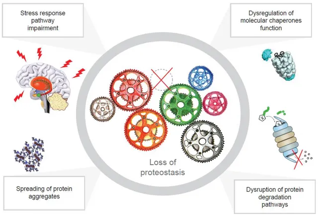
Figure 4. Mechanisms of loss of proteostasis. The disruption of the proteostasis network is generally related

to four mechanisms: the impairment of the stress response pathway, the dysregulation of chaperones, to the disruption of protein degradation pathways and also to the accumulation of aggregates.

(11)

Page | 11 In general, proteostasis network disruption has been reported to be consequence of (Figure 4):

 The dysregulation of molecular chaperones activity. Studies of chaperone levels showed that a decline in the levels of HSP70 and DNAJ/HSP40, as well as some co-chaperones correlates with protein aggregation (Hay et al., 2004; Kim et al., 2002). This suggests that perturbation of molecular chaperones may be central to global proteostasis collapse under pathological conditions;

 The disruption of protein degradation pathways. One of the principal features of protein folding diseases is the ubiquitination of proteins which are contained in aggregates; the presence of inclusions that are ubiquitinated suggests that disease-related proteins marked for degradation may be inefficiently targeted to proteasomes or are resistant to degradation or an impairment of the proteolytic activity of the UPS could underlie the accumulation of ubiquitylated proteins and therefore significantly contribute to multiple neurodegenerative diseases;

 The impairment of the Stress Response Pathway. Increase in the dysregulation of the heat shock response (HSR) during disease progression has been observed to be associated with toxicity not only in tissue culture, D. melanogaster and mouse models, but also in mammalian cells (Chan et al., 2011; Olzscha et al., 2011). Few studies have investigated the relationship between the UPR pathway and neurodegenerative diseases, although several groups have reported that ER stress is an early feature of neurodegenerative and prion diseases (Hetz and Mollereau, 2014). Disruption of the ATF6 arm of the UPR response is reported “to occur in mouse models of HD and a cell model of ALS based on expression of the disease gene VAPB”, suggesting that differential changes in UPR arms may be a feature of disease progression (Gkogkas et al., 2008; Fernandez-Fernandez et al., 2011);

 Spreading of protein aggregates. The spreading of aggregates was originally demonstrated for Prions. In addition to disruptions in the proteostasis network, several observations indicate that mutant aggregates show a spreading behaviour in cultured cells, but also in rodent and patient brains. Although the spreading of aggregates appears to be a common feature of these diseases, “the mechanism by which internalization and transmission occur may be disease specific and has been proposed to occur through endosomal pathways, secretory vesicles, and macropinocytosis in models of PD, HD, and ALS, respectively”;

(12)

Page | 12 Frequently, cells may be able to adequately handle aberrant protein species for long periods, sometimes decades, as suggested by the fact that even the inherited forms of neurodegenerative disease, such as HD, do not show a clinical phenotype until advanced age.

Indeed, specific modulation of PN components can impact both aggregate morphology and lifespan in model systems, paving the way for therapeutic intervention (Balch et al., 2008; Powers et al., 2009). Expression of chaperones and co-chaperones of different classes have consistently resulted in a decrease in disease-aggregate toxicity and even increased lifespan (Auluck et al., 2002; Hoshino et al., 2011; Chafekar et al., 2012). Analogous to cellular stress responses, strategies for therapeutic treatments for neurodegenerative diseases that are associated with protein aggregation have focused on preventing the increase in misfolded entities, stabilization of the properly folded ones, and clearance of existing aggregates (Balch et al., 2008; Calamini et al., 2011). Indeed, small molecules that prolong translation attenuation on stress, and which also stabilize mutant proteins against aggregation, have been identified (Tsaytler et al., 2011), such as transthyretin. Other molecules previously found are related to folding and trafficking defects in specific disease associated proteins, such as mutant cystic fibrosis transmembrane conductance regulator (Baranczak and Kelly, 2016), and increase the degradation of toxic protein species through activation of the UPS (Lee et al., 2010) or autophagy (Sarkar et al., 2009). Because of the broad range of components which are captured by protein aggregates, improvement of the activity of endogenous stress-response pathways has been particularly useful in extending lifespan and health of the proteostasis network (Sittler et al., 2001; Mu et al., 2008; Akerfelt et al., 2010; Kumsta et al., 2017).

2. Nothobranchius furzeri: an emerging model for aging

research

(13)

Page | 13 Annual killifish are a group of teleost fishes from the cyprinodont clade, a taxon with Gondwanan distribution; they belong to the Cyprinodontiforms order, which comprises small fishes which regularly occupy marginal habitats, often inhospitable for other teleost species (Naiman, Gerking and Ratcliff, 1973; Taylor et a., 2008).

Most of the African annual killifishes belong to the genus Nothobranchius, which contains over 60 species (Froese and Pauly, 2014).

Figure 5. Sexual dimorphism in N.furzeri (modified from Cellerino, Valenzano & Reichard, 2016). Adult

males of (A) red and (B) yellow morphs, and (C) female.

African annual killifishes are small and characterized by marked sexual dimorphism and dichromatism: males are robust and colourful while females are dull. The colour of the male is sexually selected and species-specific (Haas, 1976; Wildekamp, 2004). Males of multiple species, including N.furzeri, can happen in two or more colour forms that are sympatric or allopatric. In N.furzeri, red and yellow morphs are present, differing mainly in the colouration of the caudal fin (Figure 5). Female Nothobranchius are always smaller than males, their fins are translucent and the body is pale brown.

The distribution of the genus goes from Sudan (North Africa) to KwaZulu Natal in South Africa (Wildekamp, 2004), and is composed by four different phylogenetic clades that are “almost exclusively allopatric” (Dorn et al., 2014; Cellerino, Valenzano & Reichard, 2016; Figure 6):

(14)

Page | 14  The southern clade is distributed in the southern part of the Zamberi River, going from the

humid coast to dry habitats, and has also been the most studied;

 The inland clade is distributed in a region at high altitude between Lake Victoria (Uganda) and Kafue basin (Zambia) and is separated from the coastal clade by rift valleys;

 The coastal clade is distributed in basins of the coast of Southern Kenya, Tanzania and Northern Mozambique.

In the genus Nothobranchius, N.furzeri has been particularly studied: it goes from the area between the Save river and the Lebombo ridge. The type locality is the Sazale Pan (Gonarezhou National Park), Zimbabwe, where the species was first collected in 1968 (Jubb, 1971). Its range encompasses a strong cline of aridity and rainfall unpredictability (Cellerino, Valenzano & Reichard, 2016; Terzibasi Tozzini et al., 2013).

Figure 6. Localization of Nothobranchius genus

across Africa (Cellerino, Valenzano & Reichard, 2016).

The most arid weather conditions are found in the hinterland, at higher altitude and furthest from the ocean; the region has irregular precipitations and is subject to stronger evaporation (Mazuze, 2007; Terzibasi et al., 2008).

Nothobranchius, including N.furzeri, normally feed on macroinvertebrates; on the taxonomic point of view, their diet is opportunistic and depends on prey availability (Polacik and Reichard, 2010). All Nothobranchius tend to be generalist predators; captive N. furzeri, like other species of the same genus, quickly eat live and frozen dipteran larvae of the genera Chironomus and Chaoborus (Genade, 2005), Live Tubifex sp. (Oligochaeta), Artemia salina and Daphnia spp.

(15)

Page | 15 The ability of Nothobranchius embryos to enter diapause seems to be an ancient character state that has been lost multiple times during the evolution of African and Neotropical killifish clades (Murphy and Collier, 1997; Hrbek and Larson, 1999).

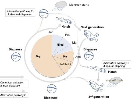
After the flooding of the pools, eggs hatch and the juveniles fishes can develop quickly in order to to reach sexual maturity. The duration of the habitat is normally of 2-3 months (Terzibasi Tozzini et al., 2013; Vrtilek et al., 2018a) and eggs stay in diapause for 10 months (as shown in the canonical developmental pathway, Figure 7); some embryos do not enter into diapause and go through direct development, hatching if the habitat is filled again during the same season (alternative pathway), otherwise they die. Some eggs have to remain in diapause for longer than one year in order to survive the occasional dry years. Variability of the diapause period length can represent an important strategy to survive an unpredictable environment (Polacik et al., 2014). After hatching juveniles are at once able to feed actively, and, under natural conditions, they can reach sexual maturity in about 12 days (Vrtilek et al., 2018b).

Figure 7. Schematic representation of the life cycle of Nothobranchius (Cellerino, Valenzano & Reichard,

2016), containing the canonical pathway (annual diapause) as well as the alternative pathways.

Several species of the Nothobranchius genus have been studied in captivity and all show short captive lifespan varying between 3 and 18 months (Valdesalici and Cellerino, 2003; Lucas-Sanchez et al., 2011; Baumgart et al., 2015).

(16)

Page | 16 Given the extremely short lifespan of Nothobranchius, and in particular N.furzeri, as compared to other vertebrates, an important part of studies in this species was focused on the confirmation that the short lifespan was a consequence of accelerated aging. Old N.furzeri shows a typical phenotype of emaciation, spinal curvature, and reduced colouration in males (Figure 8), known to be present also in Danio rerio and Oryzias latipes (Gerhard et al., 2002; Hatakeyama et al., 2008). At the behavioural level there is a generalized reduction in spontaneous locomotor activity, with older N.furzeri individuals which spend less time exploring, in comparison to young ones (Genade et al., 2005); this phenotype was reported also in N.korthausae, in addiction to the disruption of the circadian rhythm (Lucas-Sanchez et al., 2011). N.furzeri shows an impairment of learning performance during ageing, in particular when tested using an active avoidance task: the performance of older individuals in associating a conditioned stimulus with an unconditional stimulus was significantly lower than the one of younger animals (Valenzano et al., 2006; Tezibasi et al., 2008).

Histopathological examinations have revealed age-related decay of organs (Di Cicco et al., 2011). Post-mortem analyses revealed mainly lesions in kidney (Figure 8), liver and heart. Kidneys normally suffer tubule dilatation and crystal deposition (Di Cicco et al., 2011), which are present also in the human geriatric phenotype (Silva, 2005), while cardiac lesions included hypertrophy of the cardiomyocytes (another typical aspect of vertebrate ageing; Woodhead, 1984; Dai et al., 2012).

(17)

Page | 17

Figure 8. Aging phenotype of N.furzeri (Cellerino, Valenzano & Reichard, 2016; Di Cicco et al., 2011).

(A) Representation of the aging phenotype, with discolouration and emaciation of the older individual. (B-C) Liver histopathological phenotype, in particular (B) hepatomas and (C) hepatocarcinomas (both lighlighted by white arrows and dotted lines). (D-E) Kidney histopathological phenotype, in particular (D) nephrocalcinosis (indicated by white arrows) and (E) neoplasias (highlighted by dotted lines).

Cellular ageing has been deeply investigated in liver, skin and brain of several Nothobranchius species. Age-dependent accumulation of lipofuscin was observed in the liver also of wild Nothobranchius spp. (Terzibasi Tozzini et al., 2013); lipofuscin is an auto fluorescent pigment that accumulates with age in many organisms from nematodes to humans and is a key point for ageing intervention studies (Valenzano et al., 2006a; Hsu and Chiu, 209; Terzibasi et al., 2009; Yu and Li, 2012). In the liver, increased apoptosis is observed during aging of N.furzeri and also medaka (Di Cicco et al., 2011; Ng’oma et al., 2014; Ding et al., 2010).

In the skin, there is evidence that ageing is associated with accumulation of cells that may have irreversibly lost their capacity of entering the cell cycle: human senescent cells can be identified in vivo by the expression of β-galactosidase (β-Gal) marker. Age-dependent increase of β-Gal staining has been reported in N.furzeri and other two Nothobranchius species (Genade et al., 2005; Hsu et al., 2008; Liu et al., 2012) as well as up-regulation of the cell-cycle inhibitor CDKN1A.

N.furzeri brain was studied in relation to its morphology and gene expression patterns, as reported by D’Angelo et al., 2012, 2014; D’Angelo, 2013. The major cellular phenotypes that have been observed in ageing are the following:

- the important reduction of stem cell activity, observed by Tozzini et al.(2012), which accompaines the age-dependent reduction of adult neurogenesis described in mammals (Kempermann, 2011);

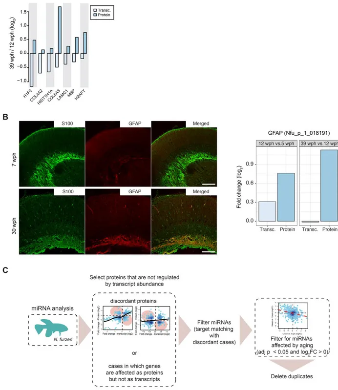
- glial hypertrophy or gliosis, as over-expression of glial fibrillary acidic protein (GFAP) (Tozzini et al., 2012), another typical phenotypic response of mammalian glia to injury,

(18)

Page | 18 neurodegenerative disease and ageing (Norton et al., 1992, Bronson, Lipman and Harrison, 1993);

- neuronal degeneration, as measured by Fluoro-Jade B staining in N.furzeri and N.guentheri (shown by Valenzano et al., 2006b; Terzibasi et al., 2009; Liu et al., 2012);

- accumulation of lipofuscin (Terzibasi et al., 2009; Terzibasi Tozzini et al., 2013).

At a molecular level, the major changes described in Nothobranchius species are:

- telomere erosion, observed in three different species and multiple organs (Hsu et al., 2008; Hartmann et al., 2009; Liu et al., 2012);

- reduced mitochondrial DNA quantity and mitochondrial function of the muscular mitochondria (Hartmann et al., 2011);

- Reduction of polyunsaturated fatty acids that are peroxidation-sensitive (in N.korthausae; Lucas-Sanchez et al., 2011) and modulation of mitochondrial fatty acid contents (N.rachovii), in relation to the increased damage to mitochondrial lipids (Lucas-Sanchez et al., 2014).

2.3. Genetic differences of lifespan across Turquoise killifish species

For my work, I decided to focus on N.furzeri: median lifespan in this species can be of 3 months for the Gonarezhou (GRZ) inbred strain (Valdesalici and Cellerino, 2003). Records for wild-derived strains from semi-arid or more humid regions in Mozambique (e.g., MZM-0403 and MZM-0410) and also a locality at the borderland between Mozambique and Zimbabwe (MZZW-0701) within less than 30 km from the collection point of the GRZ strain have a longer median lifespan of ~6-8 months and maximum lifespans exceeding one year (Terzibasi et al., 2008, Tozzini et al., 2013; Baumgart et al., 2016; Blazek et al., 2016); these observations suggest that the short lifespan of the GRZ strain is an extreme phenotype within the N.furzeri species itself and raises the question as to whether it is the result of captive breeding rather than a natural phenotype. Indeed, the strains cited above were established only several years ago and are genetically heterogeneous to various extents, whereas GRZ is highly inbred (Reichwald et al., 2009; Table 1). The females are entirely inbred (with a 100% homozygosity in 152 tested microsatellite markers) and males show heterozygosity exclusively at the sex-linked markers, as reported by Valenzano et al. (2009) and confirmed by Kirschner et al., where the average heterozygosity was found to be 0.01 (Kirschner et al., 2012). Genetic mapping studies did not detect a single locus of major effect for lifespan determination, suggesting its complex multigenic nature and excluding the possibility of it as result of a single recessive mutation (Kirschner et al., 2012; Valenzano et al., 2015).

(19)

Page | 19

Table 1. Genotypes of microsatellites analyzed in N. furzeri strains GRZ and MZM-0403 and the closely

related species N. kunthae (from Reichwald et al., 2009).

The extreme short lifespan observed in the GRZ strain has been shown experimentally to be coupled with an accelerated aging profile: a point of particular interest that has been studied is age-dependent neoplasia. Tumour onset is an age-dependent feature in humans, but in teleosts it is rare; on the other hand, a high incidence of spontaneous neoplasias in liver and kidney was observed in N. furzeri (Di Cicco et al., 2011). The onset of liver neoplasias was dependent on the longevity of the strain, and it was accelerated in the GRZ. Age-related histological markers have also been investigated in GRZ, as well as wild-derived strains (MZM-0403 and MZM-04010): lipofuscin accumulation in liver and brain was shown to be accelerated in the GRZ strain in comparison to the age-matched MZM-0403 animals, and also neurodegeneration was more pronounced.

(20)

Page | 20

2.4. Wild populations: growth and mortality

Captive conditions are very different from those in the wild environment, and important factors such as stress, diet composition and predator absence may affect ageing. All these parameters certainly influence gene expression. Although such differences are unavoidable, their identification is mandatory in order to generalize conclusions based on analysis of captive specimens, put them into evolutionary and natural-history perspectives and frame their interpretation. RNA-seq studies of age-associated gene expression in the wild are currently available only for bats (Huang et al., 2019) and wolves (Charruau et al., 2016). Remarkably, no datasets are available for wild populations of mice, fruit flies or nematode worms that represent the models of choice for experimental studies of aging. Food availability and taxonomical diversity of prey, but also oscillations of environmental temperature, individual interactions and sex differences in survival are the more observed differences between wild and captive populations of N.furzeri (as well as other Nothobranchius species).

Food availability in the laboratory is normally discontinuous during the day, depending on the facility operator, while wild fishes tend to eat throughout the day: in addiction, the wild consumes different types of food (Polacik and Reichard, 2010) compared to the uniform diet used in captivity. Possibly as a result of different diets, growth rates of wild N. furzeri are remarkably higher than in captivity (Blazek, Polacik & Reichard, 2013).

Water temperature vary diurnally in the wild with a maximum amplitudes of 15°C (Reichard et al., 2009), inducing important changes in gene expression patterns (Podrabsky and Somero, 2004); while temperature fluctuation is buffered in larger and deeper habitats (Figure 9), N.furzeri often inhabit narrow pools which are exposed to extreme fluctuations in environmental temperature.

(21)

Page | 21

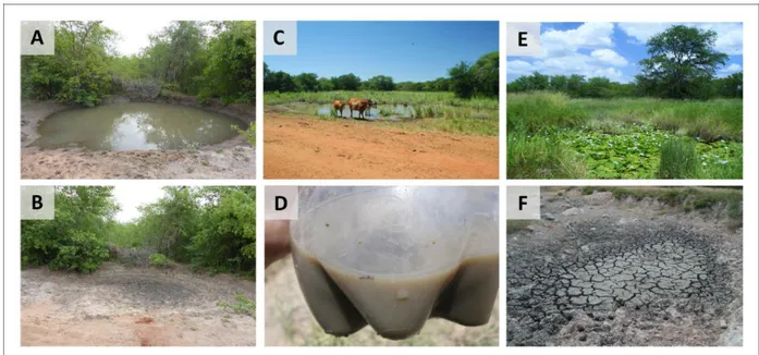
Figure 9. Natural habitat of N.furzeri (from Reichard & Polacik, 2019). (A) Habitat of N.furzeri one week

after filling with water. (B) Photo of the same habitat three weeks after (A). (C) Domestic cattle that normally visits N.furzeri habitats. (D) Turbid water from N.furzeri habitat discoloured by dissolved fine sediment particles. (E) Complex habitat with aquatic vegetation. (F) Desiccated pool sediment.

Social structure in the laboratory populations is relatively stable, since each organism has opponents or sexual partners that are fewer, in comparison to the wild environment; however, these differences are not dramatic between captive and wild populations.

Another important point to discuss is natural mortality: the most striking difference between wild and captive populations in this case is the selective mortality of wild males, not observed in the laboratory (Reichard et al., 2014). Higher extrinsic mortality, which is the mortality related to external factors such as predation, implies that fewer individuals survive to reproduce at later ages, with a subsequent weaker selection for longevity; high extrinsic mortality should then result in a rapid and dramatic ageing phenotype, as deterioration of vital function, as postulated by classical theories (Medawar, 1952; Williams, 1957; Kirkwood, 1977). Inter-sexual differences in mortality rates in wild populations are linked to extrinsic mortality; in particular increased male mortality clearly arises from that (most likely predation; Haas, 1976; Reichard et al., 2014). In a population the sexes may differ in the “relative importance of intrinsic and extrinsic mortality, making inter-sexual comparison in ageing and survival a possible avenue for ecological tests of survival” (Cellerino, Valenzano & Reichard, 2016).

(22)

Page | 22

3. High-throughput techniques for quantification of

biomolecules

3.1. Transcriptomics

3.1.1 Generalities

Transcriptome analysis technologies are the techniques used to study an organism’s transcriptome, which corresponds to the set of all of its RNA transcripts. Sequencing-based techniques can be used both to identify transcripts in an unbiased way and to quantify their abundance. A transcriptome sequencing experiment therefore isolates the total transcripts present in a cell in a defined condition. The first studies on the whole transcriptome began in the early 1990s, and technological advances since then have made transcriptomics a widely known methodology. There are two key techniques in the field nowadays: microarrays, which quantify a set of sequences which are predetermined, and RNA sequencing (RNA-seq), which uses high-throughput sequencing in order to obtain the number of counts of all expressed genes.

The measure of the expression of an organism’s transcriptome in different tissues, conditions, or at different ages gives information on how genes are regulated and reveals details of the organism itself. It can also help to guess the functions of genes that are not yet annotated. Transcriptomic analysis has allowed the study of gene expression changes in different organisms and has been a key point in the understanding of the molecular basis of human diseases.

3.1.2. Data gathering

RNA-seq

All gene expression data analyzed for this thesis originate from RNA-seq, therefore this technique will be presented here in detail.

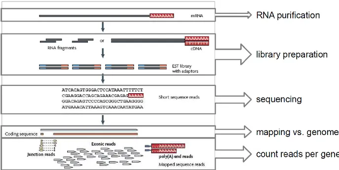
RNA-Seq refers to the “combination of a high-throughput sequencing methodology with computational methods to capture and quantify transcripts present in an RNA extract” (Figure 10) (Lowe et al., 2017; Ozsolak and Milos, 2011). The nucleotide sequences that are generated are

(23)

Page | 23 normally around 100 bp in length, but can range from 30 bp to over 10,000 bp, depending on the sequencing method which is used. RNA-Seq is based on the alignment of reads to a reference genome or to each other, in order to reconstruct the original RNA transcript (Wang, Gerstein and Snyder, 2009). The typical range of 7 orders of magnitude for RNA-Seq is an important benefit over microarray transcriptomes. In addition, input RNA amounts are much lower for RNA-Seq (ng) in comparison to microarrays (mg), which allow a more detailed examination of cellular structures and down to the single-cell level (Hashimshoni et al., 2012). Theoretically, there is no upper limit of quantification in RNA-Seq as sensitivity and precision increase by increasing sequencing redundancy, and background signal is very low for 100 bp reads in non-repetitive regions (Ozsolak and Milos, 2011). RNA-Seq can be used to identify genes in a previously annotated genome or identify which genes are active at a particular point in time, and read counts can be used to see the relative gene expression level. RNA-Seq methodology has constantly improved to increase throughput, accuracy, and read length. Since the first descriptions in 2006 and 2008 (Bainbridge et al., 2006; Nagalashkmi et al., 2008), RNA-Seq has been rapidly adopted and overtook microarrays as the dominant technique to quantify gene expression in 2015 (Su et al., 2014).

Figure 10. Workflow of an RNA-seq experiment, which is performed through RNA purification, library

preparation, sequencing, mapping and counting critical steps (adapted by Wang et al., 2009).

RNA-Seq was established with the rapid development of multiple high-throughput DNA sequencing technologies for the alignment of short sequences (Shendure and Ji, 2008). Before the actual sequencing steps, there are different methods for transcript enrichment, fragmentation, amplification, single or paired-end sequencing that can be considered.

(24)

Page | 24 We can increase the sensitivity of an RNA-Seq with the enrichment of particular classes of RNA that are of interest, but also deleting known abundant RNAs. We can also perform ribo-depletion to remove abundant but uninformative ribosomal RNAs (rRNAs) using specific probes. However, this method can also lead to the depletion of off-target transcripts (Lahens et al., 2014). Small RNAs such as microRNAs can be purified using gel electrophoresis and extraction.

Since mRNAs are longer than the read-lengths of typical high-throughput sequencing methods, transcripts need to be fragmented before sequencing: this is a key aspect of the construction of a sequencing library (Knierim et al., 2011). It may incorporate chemical hydrolysis, nebulization, or sonication of RNA, but also make use of simultaneous fragmentation.

During the preparation, the copies of transcripts (as cDNA) can be amplified by PCR to enrich fragments with 5ʹ and 3ʹ adapter sequences (Parekh et al., 2016). Amplification is also used to allow sequencing of very low-input amounts of RNA.

When the molecules have been prepared, they can be sequenced in one direction (single-end) or both directions (paired-end). The first method is faster and less expensive, and also sufficient for quantification of gene expression levels, but the second one produces more robust alignments and/or assemblies, important in particular for gene annotation and transcript isoform discovery (Wang, Gerstein and Snyder, 2009). Strand-specific RNA-sequencing preserves the strand information of a sequenced transcript (Levin et al., 2010): without strand information, reads do not inform in which direction the gene is transcribed. This method is really useful for taking information about transcription for genes that overlap in different directions, and to make a more robust gene prediction in non-model organisms (Levin et al., 2010).

Currently, RNA-Seq is based on the conversion of RNA molecules into cDNA molecules before sequencing, making the platforms for transcriptomic and genomic data the same (Figure 10B). Consequently, the development of DNA sequencing technologies has been a defining feature of RNA-Seq (Liu et al., 2012; Loman et al., 2012; Goodwin, McPherson and McCombie, 2016). Direct sequencing of RNA using nanopore sequencing represents a current RNA-Seq technique in its infancy (in pre-release beta testing as of 2016) (Garalde et al., 2016; Loman et al., 2015). However, this sequencing method can detect modified bases that would not be found otherwise when sequencing cDNA and eliminates amplification steps that could otherwise introduce bias (Morozova, Hirst and Marra, 2009; Ozsolak et al., 2009).

(25)

Page | 25 The sensitivity and accuracy of an RNA-Seq experiment are dependent on the number of reads obtained from each sample. A large number of reads are needed, in order to have sufficient coverage of the transcriptome, permitting the detection of low abundance transcripts. However, the most effective way to improve the detection of differential expression in genes with low expression is to add more biological replicates, rather than adding more reads (Rapaport et al., 2013).

3.1.3. Data analysis

RNA-Seq experiments allow the generation of a large number of raw sequence reads, which have to be processed to obtain useful information: this step usually requires a combination of bioinformatic tools that can be used for different aims and with different experimental designs. The process can be broken down into the following stages: quality control, alignment, quantification, detection of differentially expressed genes and clustering (Van Verk, Hickman, Pieterse and Van Wees, 2013). Most popular RNA-sequencing softwares work from a command-line interface, either in a Unix environment or within the R/Bioconductor statistical environment (Huber et al., 2015).

Quality control step

Another important step is the quality control process, where raw data are examined for the detection of errors or artifacts (Conesa et al., 2016). There are several options for sequence quality analysis, including the FastQC and FaQCs software packages (Lo CC and Chain, 2014). Abnormalities identified can be removed by trimming or tagged for special treatment.

Alignment

Normally transcripts are aligned to a reference genome, or de novo aligned to one another if no reference is available. The key challenges for this type of process includes the speed to allow more than 109_{of short sequences to be aligned in a meaningful way, the flexibility to recognize intron} splicing regions, and the correct assignment of reads that map to multiple locations. Software advances have greatly addressed these issues; a list of currently available high-throughput sequence aligners is maintained by the EBI (Fonseca, Rung, Brazma and Marioni, 2012).

Alignment of eukaryotic transcript mRNA sequences to a reference genome requires previous handling of the intron sequences, which are absent in mature mRNA. Short read aligners perform an additional round of alignments for the identification of splice junctions; the identification of intron

(26)

Page | 26 splice junctions prevents reads from being aligned in an erroneous way or discarded, permitting to more reads to be aligned to the reference genome and improving the accuracy of the estimates. In order to align reads to one another without the use of a reference genome a de novo assembly strategy can be used (Table 2A) (Miren, Koren and Sutton, 2010). An initial characterization of the N. furzeri transcriptome indeed required de novo transcriptome assembly (Baumgart et al., 2014) and transcriptome assembly was used to compared transcript sequences across Nothobranchius species differing in lifespan (Sahm et al., 2017). Once assembled de novo, the product of the process can be used as a reference for other sequence alignment methods and quantitative gene expression analysis.

Table 2. Common softwares used for alignment and differential analysis (adapted from Lowe et al., 2017). (A) Commonly used softwares for transcriptome de novo assembly. (B) Most used softwares for

detection of differentially expressed genes.

Quantification

Quantification of sequence alignments may be performed at different levels (gene, exon, or transcript). Typical outputs include a table of reads counts for each feature: gene and exon read counts can be calculated using the HTSeq software package (Anders, Pyl and Huber, 2015), and reads that align equally to multiple locations must be identified and then removed, aligned to one of the possible locations, or aligned to the most probable location.

(27)

Page | 27

Detection of differentially expressed genes

Once quantitative counts of each transcript are available, differential gene expression is then tested. Detection of differential gene expression lies at the center of RNA-seq but is non-trivial due to the specific nature of the data. The first step is the normalization that is required to correct for the fact that different samples differ in the total amount of reads analyzed. The second step is the modelling of the probability distribution function (negative binomial) that underlies actual data distribution. Since typically only a handful of samples are available these do not allow gene-specific estimates of the parameters and a priori assumptions are necessary to model data distribution and perform statistical test. Examples of dedicated software are described in Table 2B, the use of generalized mixed linear models as statistical framework has become predominant since it allows to test for the effects of different covariates and also to introduce random effects in longitudinal designs.

Most read a table of read counts as their input, but some (such as cuffdiff) accept binary alignment map format read alignments. The final outputs of these analyses are “gene lists with associated pair-wise tests for differential expression between treatments and the probability estimates of those differences” (from Wikipedia).

Gene expression clustering methods

An additional step for the inspection of the data is clustering. Several methods can be used in order to subset the data and find a structure inside them (on the assumption that genes with similar expression profiles must share similar biological properties; Cellerino & Sanguanini, 2018; Rodriguez et al, 2019).

Gene expression clustering methods focus on the partition of a group of genes into sub-sets, in order to reduce the numerosity of the data. The critical steps in this type of analysis are defining a measure of distance between the genes, apply a similarity criterion (which varies from method to method) to partition the data, and define a cluster. The four more used types of analysis are the hierarchical clustering, the k-means clustering, the fuzzy c-means clustering and the Self Organizing Maps.

- Hierarchical clustering: it organizes the dataset as a dendrogram (where the root is the whole dataset, and the branches define different clusters) and it follows three steps. The first one is the quantification of the distance between each pair of genes (or pairwise distance), which gives an upper-diagonal similarity matrix as a result. After the highest value is found the two most connected genes are grouped into one single cluster and the similarity matrix is recomputed until only the root remains.

(28)

Page | 28 - K-means clustering: it subdivides the genes into a predefined number of clusters which

centroids are randomly located (seeding step). The genes are then assigned to the closest centroid (through minimization of a distance measure) and the updated centroids are computed. The analysis is reiterated until the assignment of the genes to each cluster remains stable.

- Fuzzy c-means clustering: this method overcomes one of the limitations of k-means clustering, which is that a given gene can be included in only one cluster, and assigns to each gene a membership value (from 0 to 1) for each centroid. The algorithm continues until convergence (as in the k-means clustering).

- Self-Organizing Map: is a particular topologically-oriented 2D neural network, formed by a 2D grid of interconnected artificial neurons for mapping particular features in the dataset.

Knowledge-based clustering methods

A complementary method for the reduction of the data is the clustering of genes into given gene sets previously defined (by a priori knowledge of the function); normally this kind of analysis is particular useful when tested on an overrepresented list of genes (such as differentially expressed genes), but also to test a gene set in accordance to its up- or down-regulation to a given condition (as in the “Gene Set Enrichment Analysis” analysis).

- Gene Overrepresentation (GO analysis): this type of analysis is done comparing a gene set to a background gene list and is based on the hypergeometric distribution

where n is the total number of genes in the experimental gene set and N the total number of genes in the background list, whereas k is the number of DEGs in the experimental gene set and K the number of DEGs in the background list. The method provides also the measurement of an enrichment score, as ratio between observed frequency (n/k) and expected frequency (N/K).

(29)

Page | 29 - Gene Set Enrichment Analysis (GSEA): GSEA provides a statistical framework in order to

test whether a given set of genes is up or down-regulated in accordance to a given condition. The most used GSEA approach is called Generally Applicable Gene Enrichment (GAGE), where a meta-analysis (for the combination of different observations) is used as main approach. Given the gene set (S), the background list (B) and two individual samples, the mean and variance of all the fold changes contained in each sample are compared with a Student’s t-test, and this is repeated for all the pairwise comparisons. The process allows the measurement of the mean of log(pvalues), shown here,

and a new variable is obtained, which follows a Γ distribution, and corresponds to the enrichment of the gene set S.

3.1.4. Validation of the results

Differential expression detected by transcriptomic analyses may be validated using an independent technique, for example, quantitative PCR (qPCR), which is widely used and statistically assessable (Fang and Cui, 2011). Independent validation may entail the analysis of the same RNA samples analyzed by RNA-seq (technical validation) or of a new set of samples (biological validation). In qPCR, expression of the genes of interest is quantified relative to the expression of a control (so called house-keeping) gene. The measurement by qPCR refers to the amplification cycle when the signal becomes detectable. However, qPCR specifically targets amplicons smaller than 300 bp, usually toward the 3ʹ end of the coding region, avoiding the 3ʹ untranslated region (3ʹUTR) (Ramsköld, Wang, Burge and Sandberg, 2009) and therefore cannot be used to asses differential transcript isoforms. A key disadvantage of qPCR is that is relies on the arbitrary selection of the normalizer genes and erroneous selection of nonstable normalizers invalidates all downstream analyses. The quantification of multiple control genes along with the genes of interest produces a

(30)

Page | 30 more stable reference within a biological context as reference genes may be stable under certain conditions but not others (Valdesompele et al., 2001).

RNA-seq experiments normally suggest some functional implication of differentially expressed genes or gene sets in the biological phenomenon under study. Assessing this assumption through experimental manipulations of the expression of some key genes (functional validation) has become an almost mandatory step in transcriptome analysis. Observed gene expression patterns may be functionally linked to a phenotype by an independent knock-down/rescue study in the cells or organism of interest. Since these experiments are typically expensive and time demanding, they currently represent the bottleneck of transcriptomic studies.

3.2. Proteomics

3.2.1 Generalities

Proteomics is the study of protein products expressed by the genome, and has become one of the leading technologies in the post-genomic era due to the central role of proteins and protein–protein interactions in the cell (Tyers and Mann, 2003; Cox and Mann, 2007). The term proteomics for the global study of proteins was first coined in the early 1990s by Marc Wilkins and can be equally used with respect to a whole organism, a tissue, a biological fluid, a cell, or even an organelle (Wilkins et al., 1996a,b). Proteomics is only made possible by the coordinated integration of many fields of scientific endeavor. Most importantly, but not exclusively, these include genome sequencing, protein separation science (and protein biochemistry in general), mass spectrometry (MS), and bioinformatics, and these have been described as the four pillars on which proteomics technologies stand (Tyers and Mann, 2003).

There is growing attraction to the concept of comprehensive or system-wide analyses of proteins and the 2000s have seen tremendous advances in proteomics technologies and the quality of data produced to address this question. These technologies offer considerable opportunities for improved biological understanding of a particular system in health or disease (see Cravatt et al., 2007 for some notable examples). In addition, another major potential application of proteomics is biomarker discovery and considerable resource has been directed in this direction as well over the past decade. These advances in proteomics have taken place in coincidence with tremendous progress in all areas of functional genomics (understanding the function of genes and their corresponding proteins on a global scale). Mass spectrometry (MS) is the central technological basis of proteomics and this is

(31)

Page | 31 particular true of protein identification and quantification (Aebersold and Mann, 2003; Yates et al., 2005; Domon and Aebersold, 2006).

The first applications MS related to the identification of specific proteins but soon extended to the quantification of protein abundance. Later applications include the analysis of post-translational modifications (PTMs, such as lipid modification, glycosylation, phosphorylation, and many others), proteolytic processing, and association with other proteins or different types of molecules. All of these components are crucial for the description of biological systems but also significantly complicate the experimental analysis of proteins (Aebersold, 2003).

Protein discovery is a major opportunity afforded by proteomics technologies. This might apply to biomarker discovery in clinical contexts or the identification of new proteins of interest in basic science projects. Such protein discovery approaches also offer clear potential for the generation of new hypotheses. The technology is also suited to asking much more defined questions of a handful or even individual proteins. Protein discovery studies might arbitrarily be categorized as being comprehensive, broad scale, or focused. Comprehensive approaches are typically qualitative and are focused on the enumeration of the components of a biological system. A good example of this is the Human Proteome Organization (HUPO) Plasma Proteome Project (PPP), which aims to identify every protein in human plasma (Omenn et al., 2005). Proteomics technologies can also be used to assay specific known entities. An example of such an experiment would be the measurement of biomarker components in plasma within a clinical setting (Hoofnagle et al., 2008; Keshishian et al., 2009). These assay approaches can also be used for biomarker candidate validation and might be used for individual peptide quantification in a range of studies (Mallick and Kuster, 2010).

The field of proteomics spans a wide range of research topics and distinct approaches need to be applied depending on the question being asked. These vary widely in their versatility, technical maturity, and difficulty and, as a consequence, some questions are much harder to answer than others. Here we describe approaches for protein identification and quantification that are widely used today and reflect on the tremendous progress that has been made in these areas of analysis in the past decade.

3.2.2 Workflows for proteome quantification

Proteins are derived from entire cells or from biological fluids and the totality of the proteins can be processed (Figure 12). However, it is often preferable to perform subcellular fractionation to enrich for proteins of particular biological interest and achieve localization information. One further option with biological fluids is protein depletion in order to more readily analyze the lower abundance

(32)

Page | 32 proteins. Protein solubilization is usually performed in a single step but differential detergent solubilization is possible using detergents with different properties. Proteins can be separated by two-dimensional electrophoresis (2DE). In this workflow, an individual protein “is removed as a gel plug, trypsin digested and the resulting peptides are typically separated based on relative hydrophobicity by nanoscale liquid chromatography (LC) before tandem mass spectrometry (MS/MS)” (Labbadia and Morimoto, 2015).

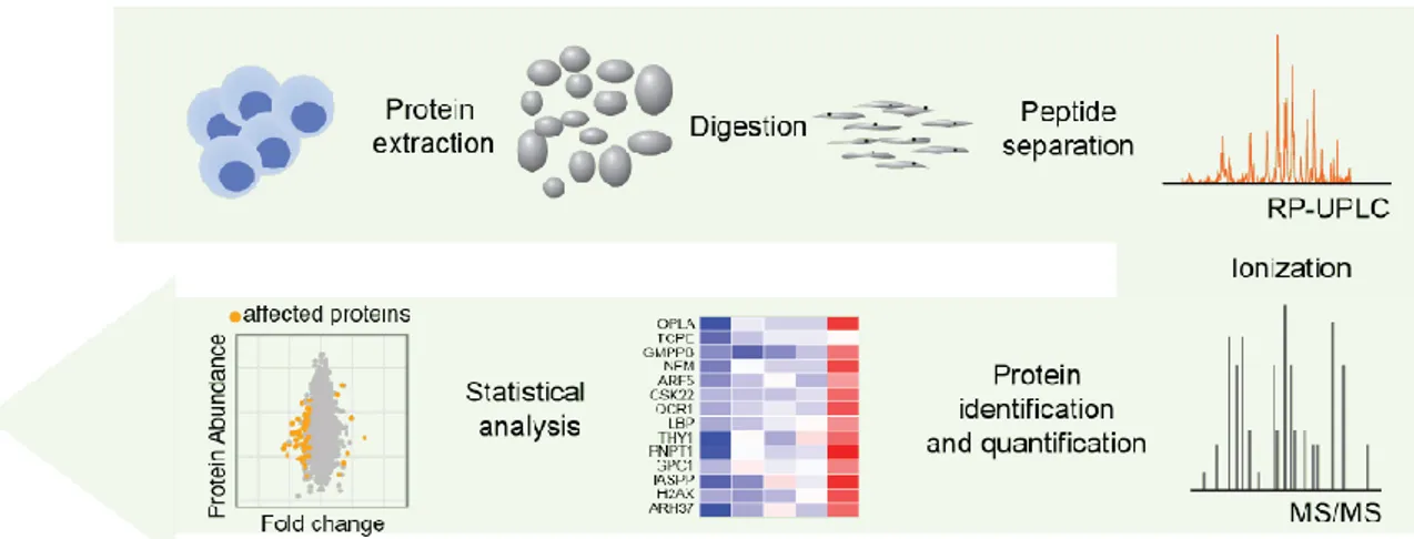
Figure 12. Typical proteome quantification workflow. A typical MS experiment consists in extraction of

proteins (from cells or tissues), protein digestion, peptide separation, ionization, protein quantification and final computational analysis.

The resulting MS data is matched to existing protein databases; the method of choice for 2DE protein quantification is difference gel electrophoresis where samples are labeled with different fluorescence substances before mixing together and 2DE. For global analysis we rather digest with trypsin the entire solubilized protein mixture. Peptides are then separated by liquid chromatography on their hydrophobicity and often charge as a multidimensional separation. Then a first MS step analyzes m/z rations in a mixture of tryptic peptides and then individual peptides are broken down to the single amino acids in the second MS step. Database searches are then performed to assign the peptide to described proteins. Based on the intensity of the signal derived from peptides of a given protein, protein abundance in the original sample can be estimated. Label-free MS quantification can also be performed using spectral counting or ion current measurements. Quantifications can be performed using internal standards in the form of labelled peptides or by metabolic labelling of the whole proteome (stable isotope labelling by aminoacids in cell culture, SILAC). The most developed technique involves the multiplexing of peptides labelled with isobaric labels (tandem mass tag, TMT)

(33)

Page | 33 that co-elute during the first MS step and can be deconvoluted in the second MS step. This latter technique is a prominent source of the data analyzed in the present thesis and is described in detail.

3.2.3 The TMT10 technique

Several labeling techniques can be used to measure the relative abundance of proteins in different biological samples by mass spectrometry. Two general labeling strategies—in vivo and in vitro labeling—have been widely applied to quantitative protein analysis. The first strategy normally uses heavy isotopes, which are then incorporated into the proteins of the organisms: this step is performed through feeding in the medium or the food (Oda et al., 1999). This approach has limitations: it requires a large amount of growth medium, and there are difficulties in the control of labeling efficiency (Thompson et al., 2003). In vitro labeling passes these limitations by chemically labeling any peptide sample with high efficiency: an example is the isotope-coded affinity tag (ICAT) technique (Gygi et al., 1999). With this method, probes that are the same on the chemical point of view, but with different masses, are used to label two peptide samples. The relative abundances are then determined from the intensities of MS1 peaks that are distinct in their mass to charge ratio (m/z). Other techniques started using isobaric tags, such as TMT and iTRAQ (Thompson et al., 2003; Ross et al., 2004): the reagents used are normally composed of a mass reporter, a mass normalizer and an amine reactive group. The first two parts are important for the incorporation of stable isotopes in multiple configurations such that each mass reporter’s mass can be seen in a MS2 spectrum. The intact mass of each isobaric tag variant, however, is the same. With this labeling strategy, digested peptides from multiple samples are first labeled in parallel, then they are then mixed and analyzed using reversed phase high performance liquid chromatograph (HPLC) coupled with a mass spectrometer capable of tandem MS analysis (Figure 13).

(34)

Page | 34

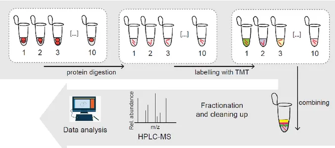
Figure 13. Workflow of TMT technique. After the first step of protein digestion, peptides are labelled and

then all the samples are combined in one tube; after fractionation and cleaning a mass spectrometry workflow is followed and the data are analysed.

The mass reporter can be divided from the peptide through collision-induced dissociation (CID) or through higher energy collision dissociation (HCD) before detection; the relative quantification of the peptide is measured as the intensity of the reported ions in the MS2 spectrum. The isobaric and chemically identical nature of isobaric tags ensure that “identical peptides labeled with different tag variants will have the same chromatographic elution profile, and experience identical ionization processes in the mass spectrometer” (Zhang and Elias, 2017), with a more accurate final quantification. Another important strength of this technique is the improvement of the signal-to-noise ratio by enabling quantification at the MS2 level, in comparison to the MS1 scan of the peptides. However, in highly complex peptide mixtures, co-isolation and co-fragmentation of multiple ions is increasingly likely to occur with MS2, resulting in distorted ratios of isobaric tag reporter ions (Ting, Rad, Gygi and Haas, 2011). Sometimes, when working with complex peptide mixtures, the co-isolation and co-fragmentation of multiple ions normally happens with MS2, with the subsequent distortion of isobaric tag reporter ions: in this case, the ratios can’t reflect anymore the true proportions of a selected peptide precursor’s components. Combining ion trap and orbitrap technologies measures reporter signals with a third stage of ion isolation and fragmentation (MS3), reducing the ratio distortion resulting from interfering ions (Ting, Rad, Gygi and Haas, 2011). Another strategy, called “MultiNotch MS3” method, was shown to increase detection sensitivity after selecting multiple fragment ions from MS2 to enhance reporter ion intensities at the MS3 level (McAlister et al., 2014).

(35)

Page | 35

3.2.4 Thermal Proteome Profiling

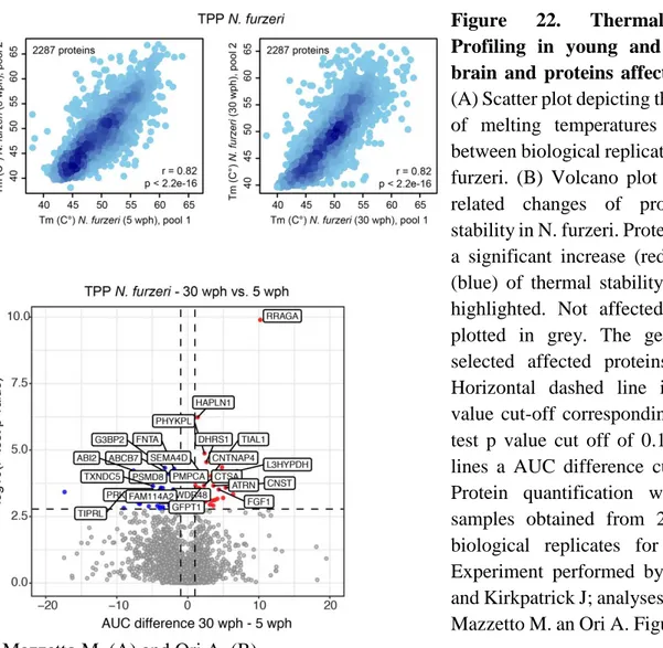
In this thesis the Thermal Proteome Profiling (TPP) technique was adopted to highlight potential differences in protein stability between young and old animals: this method focuses on the differential stability of proteins after a heat shock (assuming that proteins become more resistant to heat-induced unfolding when in complex with a ligand), can be applied on live cells and doesn’t require labelling. As shown by the principle of thermal shift assays, when proteins are subjected to a heat shock they generally irreversibly unfold (exposing their hydrophobic core and subsequently aggregating); however, their melting temperature (i.e. the temperature at which unfolding happens) can be increased after the binding with a ligand, as shown by structural biology (Vedadi et al., 2006; Ericsson et al., 2006) and drug discovery fields (Pantoliano et al., 2001; Senisterra et al., 2006).

In particular, the TPP technique combines this principle with mass spectrometry-based proteomics: the workflow of the experiment generally consists of (1) preparation of the cells for the experiment, (2) heating procedure, (3) extraction of soluble proteins, (4) protein digestion with peptide labelling, (5) mass spectrometry and (6) data processing (Figure 14).

Figure 14. (A) Principle of the thermal shift assay (adapted from Mateus, Määttä & Savitzki, 2017). (B)

General workflow of the Thermal Proteome Profile (TPP) technique.

TPP can be performed on cells extracts, intact cells or tissues: cell lysis (prior to TPP) dilutes metabolites, proteins and co-factors, in order to stop the metabolism of the cell (so that stabilization of the protein should just be the result of binding to the ligand). After this preparation, cells can be

(36)

Page | 36 incubated with a drug in order to identify candidates: the choice of using a single compound concentration or a range of concentrations is linked with the next step, the heating process.

Following the heat treatment cells are lysed and proteins that are denatured (and aggregated) are removed using ultracentrifugation (Savitzki et al., 2014); new protocols have shown that the use of mild detergents results in the inclusion of membrane proteins in the analysis without affecting heat-induced aggregation. Once the soluble proteins are collected, they are digested following a normal proteomics workflow (Figure 12) and the resulting peptides from each condition are labelled using TMT and combined into a single sample for the mass-spectrometry analysis (Figure 13).

4. N.furzeri as a model for computational genomics

approach to ageing

4.1. Genome-related studies

In the genomic era the availability of a genome reference sequence is really important for the recognition of an organism as model for scientific research. The first insights were provided by cytogenetics and genome survey Sanger sequencing (Reichwald et al., 2009); the N.furzeri genome contains 19 chromosomes and was estimated to be extremely repeat rich, particularly in satellite sequences (Figure 15). Crosses of the shortest-lived strain GRZ and more recently wild-derived strains (already mentioned in paragraph 2.3) provided the first genetic maps of the N.furzeri genome and lifespan controlling quantitative trait loci (QTLs; Kirschner et al., 2012), showing that lifespan determination is polygenic. In particular, four QTLs regulating lifespan were identified, located at linkage groups (LG) 9, 11, 14 and 17, starting from 22 LGs. Both studies identified males as the heterogametic sex, concordant with an XY sex-determining (SD) system.

(37)

Page | 37

Figure 15. Genome architecture of N.furzeri (from Platzer & Englert, 2016). (A) Composite male GRZ

karyotype. (B) Stepwise assembly of the 19 sgrs of the reference, with scaffolds obtained by sequence assembly (inner circle), super scaffolds built on integration of optical map (second circle), genetic scaffolds generated by linkage map integration (third circle), and sgrs defined on analyses of synteny in medaka and stickleback (outer circle). (C) High-density restriction-site-associated DNA (RAD) map of the 19 linkage groups.

Two independent N.furzeri genome assemblies were performed and published in parallel, thanks to the new possibilities given by modern sequencing technologies (Reichwald et al., 2015; Valenzano et al., 2015). In the first study, “to reach chromosome-scale long-range continuity, a five-step strategy was used compromising sequence assembly, scaffold/gap filling, integration of optical and genetic linkage maps, and finally comparative synteny mapping in two closely related fish species” (Platzer & Englert, 2016). The second study used RNA-seq and a high-density restriction-site-associated DNA (RAD) linkage map; this strategy resulted in an improved contiguity and the assignment of sequence scaffolds to chromosome-scale linkage groups.

The two studies succeed in finding genomic regions enriched in aging-related genes with these two complementary methods; the first used the long-range contiguity of the reference sequence and performed a genome-wide positional gene-enrichment analysis for differentially expressed genes (DEGs) in N.furzeri strains with different lifespan rates, detecting seven genome-wide positional regions. On the contrary, the second study made use of QTL mapping crossing short- and long-lived strains, identifying one genome-wide significant lifespan QTL (which was shown to be located on the sex chromosome, consistently with the previous findings reported by Kirschner et al., and was found to be enriched for known aging-related genes).

Both studies also searched their protein-coding annotations for signs of positive selection, in order to identify candidates which could lead to the short lifespan of this species, with 497 N.furzeri genes with at least one site under positive selection identified by Valenzano et al., and only seven in N.furzeri and one in N.pienarii (which shows convergent evolution of very short lifespan) by Reichwald et al.

Unraveling the molecular mechanisms of aging in Nothobranchius furzeri using high-throughput techniques

SCUOLA NORMALE SUPERIORE

MARIATERESA MAZZETTO

RELATORI

CANDIDATA

Contents

___________________________________

Introduction………p. 6

1. Aging and proteostasis

1.1. What is aging?

1.2. The proteostasis network and the proteasome-inhibited

1.3. The proteostasis network during aging

2. Nothobranchius furzeri: an emerging model for aging research

2.1. Natural history

2.2. Life cycle, lifespan and aging in N.furzeri

2.3. Genetic differences of lifespan across Turquoise killifish species-specific

2.4. Wild populations: growth and mortality

3. High-throughput techniques for the quantification of biomolecules

3.1. Transcriptomics

3.1.1. Generalities

3.1.2. Data gathering

3.1.3. Data analysis

3.1.4. Validation of the results

3.2. Proteomics

3.2.1. Generalities

3.2.2. Workflows for proteome quantification

3.2.3. The TMT10 techniques

3.2.4. Thermal Proteome Profiling

4. N.furzeri as a model for computational genomic approach of ageing

4.1. Genome-related studies

4.2. Transcriptome-related studies

4.3. MiRNome-related studies

Aim of the work………p.42

List of datasets used………..p.44

Materials and Methods………..p.45

1. Trascriptome-proteome comparison

1.1. Abundance comparisons

1.2. Differential expression analysis

1.3. Metanalysis

2. Enrichment analysis

2.1. GO analysis

2.2. Generally-Applicable Gene-Set Enrichment (GAGE)

3. MiRNA analysis

4. Loss of stoichiometry analysis

4.1. Complex analysis (Ori et al.)

4.2. IQR analysis

5. Principal Component Analysis (PCA)

6. Network Analysis

6.1. Consensus analysis on multiple datasets

7. Survival analysis

8. RNA isolation

8.1. Protocol

8.2. Recipes

9. Retro-transcription

9.1. Genomic DNA removal

9.2. Retrotranscription

9.3. Recipes

9.4. Catalog numbers

10. PCR technique

10.1. Primers used

10.2. PCR

10.2.1 Recipes

10.2.2. Catalogue numbers

10.3. Quantitative PCR

10.3.1. Recipes

11. Proteomic techniques

11.1. Sample processing for MS

11.1.1 Recipes

11.2. Data analysis

11.3. Thermal Proteome Profiling

11.3.1. Recipes

12. Cell culture

12.1. Thawing cells

12.2. Splitting cells

12.3. Harvesting cells

Results………...p.57

1. Ribosome stoichiometry loss and aggregation in the aging brain of N.furzeri

1.1. Decoupling between transcriptome and proteome during aging

1.2. Stoichiometry imbalance in protein complexes during aging

1.3. Thermal Proteome Profiling reveals minor changes in protein stability during