Galactic cosmic-ray recurrent and transient short-term variations: advanced data analysis and modeling

(1)

UNIVERSITÀ DEGLI STUDI DI URBINO CARLO BO

Dipartimento di Scienze Pure e Applicate

Corso di Dottorato in Scienze di Base e Applicazioni Curriculum di Scienza della Complessità

XXXII CICLO

Tesi di Dottorato

GALACTIC COSMIC-RAY RECURRENT AND

TRANSIENT SHORT-TERM VARIATIONS:

ADVANCED DATA ANALYSIS AND MODELING

Relatore: Candidato:

Prof.ssa Catia Grimani Simone Benella

Correlatori:

Dott.ssa Monica Laurenza Prof. Giuseppe Consolini

Settore Scientifico Disciplinare: FIS/01

(2)

(3)

Alla mia famiglia.

(4)

(5)

Publications

Grimani, C., Telloni, D., Benella, S., Cesarini, A., Fabi, M., & Villani, M. (2019). Study of Galactic Cosmic-Ray Flux Modulation by Interplan-etary Plasma Structures for the Evaluation of Space Instrument Perfor-mance and Space Weather Science Investigations. Atmosphere, 10(12), 749.

Benella, S., Grimani, C., Fabi, M., Finetti, N., & Villani, M. (2019).

Recurrent and non-recurrent galactic cosmic-ray flux short-term varia-tions observed with LISA Pathfinder. In 36th International Cosmic Ray Conference (ICRC2019) (Vol. 36).

Benella, S., Grimani, C., Laurenza, M., & Consolini, G. (2019).

Grad-Shafranov reconstruction of a magnetic cloud: Effects of the magnetic-field topology on the galactic cosmic-ray intensity. Nuovo Cimento C Geophysics Space Physics C, 42.

Grimani, C., Telloni, D., Villani, M., Finetti, N., Laurenza, M., Benella,

S., & Fabi, M. (2019). Galactic cosmic-ray flux short-term variations and

associated interplanetary structures with LISA Pathfinder. Nuovo Cim., 42, 42.

Armano, M., Audley, H., Baird, J., Benella, S., Binetruy, P., Born, M., ... & Cruise, A. M. (2019). Forbush decreases and ă 2 day GCR flux non-recurrent variations studied with LISA pathfinder. The Astrophysi-cal Journal, 874(2), 167.

Armano, M., Audley, H., Baird, J., Bassan, M., Benella, S., Binetruy, P., ... & Cruise, A. M. (2018). Characteristics and energy dependence of recurrent galactic cosmic-ray flux depressions and of a forbush decrease with LISA Pathfinder. The Astrophysical Journal, 854(2), 113.

(6)

Entropy, 19(8), 383.

Grimani, C., Benella, S., Fabi, M., Finetti, N., Telloni, D., & LISA Pathfinder Collaboration. (2017, May). GCR flux 9-day variations with LISA Pathfinder. In Journal of Physics: Conference Series (Vol. 840, No. 1, p. 012037). IOP Publishing.

(7)

Acknowledgments

I would like to express my gratitude to my supervisors Professor Ca-tia Grimani and Dr. Monica Laurenza. They guided me, for the first time in my career, in the magic world of cosmic rays sharing with me their precious knowledge. I will never thank them enough for their avail-ability and for all the opportunities that they gave me during my PhD course. I wish to acknowledge my third supervisor Professor Giuseppe Consolini that introduced me to the physics of complex systems being an inestimable guide during the years 2014-2020.

Special thanks go to Professor Rami Vainio and Dr. Alexandr Afanasiev of the Department of Physics and Astronomy of the University of Turku (Finland) for extensive discussions and valuable suggestions which greatly contributed to the improvement of this thesis work. They hosted me for a visiting period, supporting my work with enthusiasm and helping me to widen my research from various perspectives.

I would like to render my warmest thanks to Professor Qiang Hu at the Center for Space Plasma and Aeronomic Research at the University of Huntsville in Alabama (UAH, AL, USA) for his precious help and for having shared with me his knowledge and his computer codes. I thank him very much especially for his availability and kindness.

I would like to express my gratitude to the director of my PhD cur-riculum, Professor Vincenzo Fano for sharing with me his deep passion and knowledge on fundamental of physics. This thesis has been written during my stay at the Department of Pure and Applied Sciences at the University of Urbino and I would like to thank the directors of my PhD course, Professor Mauro Sergio Micheloni first and Professor Alessandro Bogliolo at present time, for providing excellent working conditions and financial support for my research traveling.

I would like to thank the National Institute for Nuclear Physics in Florence and the Institute for Spatial Astrophysics and Planetology in Rome for the financial support for traveling abroad to attend interna-tional conferences, summer schools and visiting periods.

(8)

and Dr. Andrea Cesarini for his precious work on the LISA Pathfinder platform magnetic field data and unforgettable moments spent together. I would like to thank all the people at the Institute for Spatial Astro-physics and Planetology in Rome, in particular my office mate Virgilio Quattrociocchi that shared with me two amazing summer schools and Tommaso Alberti for all the interesting and constructive discussions. I would like also to thank all the colleagues at UAH, where I spent two months, in particular Bishwas Shresta for being an excellent physicist and a great friend.

I would like to thank my “Chérie”, Maria Chiara for being part of my life, for encouraging me and loving me everyday and, last but not least, I wish to express my gratitude to my family, my brother Luca, my mother Mara and my father Piero for their important support during my life and scientific career: I acknowledge to them the achievement of this objective.

Simone Benella

(9)

List of Figures

1 Sketch of the cosmic-ray propagation from the interstellar medium through heliosphere, magnetosphere and interac-tion with the Earth atmosphere. . . 2 1.1 Left: sketch of the LPF satellite. The figure shows the

two TMs (TM1 and TM2) and two independent interfer-ometers allowing for positioning the TMs with respect to the satellite and among them along the experiment sensi-tive axis. Electrodes for TM actuation and electrostatic positioning are also shown (Armano et al., 2016). Right: monthly-averaged sunspot number during the solar cycle N. 24. Vertical dashed lines indicate the LPF mission elapsed time. . . 2 1.2 LPF orbit in a synodic (corotating) frame having the Earth

as the origin. The x-axis points along the direction to-wards the Sun and the x-y plane lies on the ecliptic. The

z-axis is chosen to form a right-handed coordinate system

(Landgraf et al., 2005) . . . 3 1.3 Sketch of the PD shielding copper-box and silicon wafers.

On the right is reported the PD model used for the GEANT4 simulation (Mateos et al., 2010). Simulations of the PD performance were also carried out with Fluka (Grimani and Vocca, 2005; Grimani et al., 2009). . . 4 1.4 A schematic view of the LTP with indicated

magnetome-ters location (MX, MY, PX, PY) within the LPF S/C with respect to the TM electrode housing (adapted from Diaz-Aguilo et al.,2011). . . 5 2.1 GCR energy spectra measurements from various

experi-ments, from http://www.physics.utah.edu/~whanlon/

spectrum.html. . . 7

(12)

over the termination shock (at „ 100 AU from the Sun) and are bounded by the heliopause. The trajectories of GCRs entering the heliosphere are also shown (adapted

from https://commons.wikimedia.org/wiki). . . 9

2.3 Sketch of the HCS configuration (adapted fromJokipii and Thomas, 1981). . . 11 2.4 Effective cutoff rigidity map for quiet conditions (top panel)

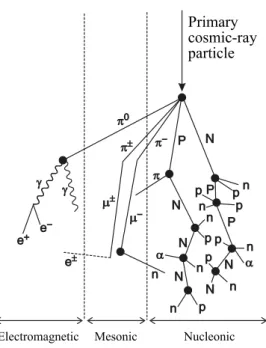
and during a geomagnetic disturbance (bottom panel). Rigidity values are given in GV. . . 15 2.5 Scheme of the cosmic-ray cascading in the atmosphere.

Symbols used are: n, neutron, p, proton (capital letters indicate particles produced in nuclear processes), α, alpha particle, e˘, electron and positron, γ, gamma rays, π, pion,

µ, muon (adapted fromDunai, 2010). . . 16

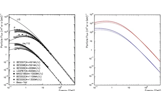
3.1 Example of GCR proton flux parameterization at 1AU. The dashed line represents the LIS proton spectrum de-fined in equation (3.4), while the solid line is the modu-lated spectrum on the basis of equation (3.3) where a solar modulation parameter φ “ 500 MV is considered. . . . . 22 3.2 Left: GCR proton and helium energy spectra

measure-ments and parameterizations. The solar modulation pa-rameter φ estimated for each set of measurements is re-ported in the legend. Observations were gathered during different solar activity and both positive (open symbols) and negative (solid symbols) polarity periods. The top curve corresponds to the LIS spectrum by Shikaze et al. (2007). The continuous middle and bottom curves corre-spond to φ “ 490 MV and φ “ 1300 MV respectively, from (Grimani, 2007b). Right: GCR proton (red curves) and helium (blue curves) fluxes. Top continuous curves corre-spond to observations gathered at solar minimum during positive polarity periods. Bottom dashed lines represent the maximum effect of the drift process during negative polarity periods (Boella et al., 2001). . . 23

(13)

3.3 Oulu NM GCR count-rate variations (black line) com-pared to the observed sunspot number (red line). Pos-itive (A ą 0) and negative (A ă 0) polarity periods are indicated on the top of the figure. Vertical dashed lines de-limit periods of not well-defined GSMF polarity according to Laurenza et al. (2014) and http://www.solen.info/

solar/polarfields/polar.html. . . 24

3.4 Sketch of two high-speed streams corotating with the Sun, showing the formation of CIRs. Dashed lines represent flow streamlines in the slow and fast solar wind. Be-low typical changes in solar wind parameters at 1 AU corresponding to the indicated regions are listed. Cor-responding GCR flux variations are also shown at the bottom of the figure. The regions indicated on the top of the figure are S: ambient, slow solar wind; S1:

com-pressed, accelerated, slow solar wind; F1: compressed,

decelerated, fast-stream plasma, and F : ambient, undis-turbed, fast-stream plasma. Forward and reverse shocks are also shown. (Richardson, 2004). . . 26 3.5 Sketch of a large-scale structure of an ICME with shock

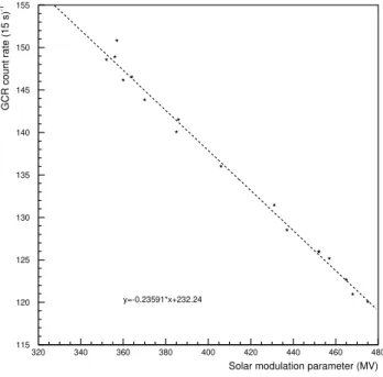
and turbulent sheath ahead. Two S/C paths through the structure are indicated as an example. The resultant cos-mic ray profile depends on the part of the structure ex-plored by the S/C. The time of shock transit S is indi-cated by a vertical solid line and the start and end times of ICME passage are indicated by vertical dashed lines. Only if the ICME is intercepted the two-step FD can be observed (Richardson and Cane,2011). . . 28 4.1 LPF PD GCR single count rate averaged over each BR

during the LPF mission versus the solar modulation rameter. High (low) values of the solar modulation pa-rameter correspond to mission beginning (end). . . 33 4.2 Hourly-averaged 15 s LPF PD count rate between

Febru-ary 18, 2016 and July 3, 2017. . . 34 xiii

(14)

´Bx (third panel), and IMF intensity (fourth panel)

con-temporaneous measurements are also shown. In the third panel the continuous line indicates HCS crossings and the sector daily polarity (positive and negative polarities were set respectively to `10 and ´10 arbitrarily in the plot). Periods of time during which the solar wind speed V , and the magnetic field B, intensity remain below and above 400 km s´1 and 10 nT, respectively, are shown in the

sec-ond and fourth panels. Decrease, plateau, and recovery periods of each GCR depression are represented by red, blue, and cyan lines, respectively, in the first panel (Ar-mano et al., 2018). . . 36 4.4 Comparison of LPF PD count rate variations with

con-temporaneous, analogous measurements of polar neutron monitors during the BR 2491 (March 4-31, 2016; Armano et al., 2018). . . 37 4.5 Intrinsic mode functions and residue from the EMD of the

LPF PD dataset (time label format is yy/mm). . . 46 4.6 Left: Energy associated with the intrinsic mode functions

as a function of their mean period. The solid line is the energy-period dependence for the Gaussian white noise and the dashed line are the first and 99th percentiles calcu-lated from equation (4.1). Right: Percentage energy level of each intrinsic mode function with respect to the total energy of the signal (first column of the histogram). The red dashed line represent the 5% threshold. . . 47 4.7 LPF GCR dataset (gray dashed line) compared to the

denoised signal obtained by summing up intrinsic mode functions 6-11 (black solid line). . . 48 4.8 Comparison between the residue of the EMD and the

13-month smoothed 13-monthly total sunspot number. . . 49 4.9 PDF ppfq of the instantaneous frequencies of the LPF

dataset. . . 50 xiv

(15)

4.10 Time-frequency diagram of the Hilbert spectrum for the LPF dataset. Horizontal dashed lines represents the typi-cal frequencies related to the solar rotation period: 27 days (red), 13.5 days (white) and 9 days (green). The white vertical dotted lines mark the edges of the BRs while dots indicate the passage of recurrent disturbances according to Table 4.3. The color map indicates the logarithm of the square amplitude of each intrinsic mode function as a function of frequency and time. . . 51 4.11 Same as Figure 4.3 for the BR 2492 (March 31-April 26,

2016; Armano et al., 2019). . . 52 4.12 Same as Figure 4.4 for the BR 2492 (March 31-April 26,

2016; Armano et al., 2019). . . 53 4.13 Magnetic field, solar wind and GCR data from July 19,

2016 through July 24, 2016. From top to bottom: IMF magnitude B, IMF GSE latitude θ, IMF GSE longitude

φ, with a smoothed solid line overlaid, solar wind speed V, plasma temperature T , GCR percentage flux variations

gathered by LPF compared to four NMs. . . 56 4.14 Same as Fig. 4.13 for the period August 2-4, 2016. . . 57 4.15 Same as Fig. 4.13 for the period May 27-30, 2017. . . 58 5.1 Cartoon presented in Prof. Sonnerup’s Van Allen Lecture

at the 2010 AGU Fall Meeting (New Yorker Magazine,

available fromhttp://www.newyorker.com/cartoons/a15439). 62 5.2 Data gathered in the Lagrange point L1 with the Wind

satellite and the LPF PD on magnetic field, plasma (panels 1-4) and cosmic-ray (bottom panel) observations during August 2-3, 2016. The MC transit time is represented by vertical dashed lines. . . 72 5.3 Scatter-plot of the convection electric field Ec“ ´vpmqˆ

Bpmq versus the HT electric field E

HT “ ´VHT ˆ Bpmq for constant HT velocity (cyan dots) and constant HT acceleration (black dots). . . 73 5.4 Magnetic hodograms for MC crossing by Wind on August

2, 2016, 20:11 UT - August 3, 2016, 02:54 UT. Axes units are in nT. Eigenvalue ratios are reported on top of the figure. 73

(16)

the S/C measurements for the first half (circles) and for the second half (stars) of the MC crossing. Solid curve represents the fitting function, PtpAq. The fit residue is

Rf “ 0.05 for this event and Ab “ ´44.7 Tm denotes

the boundary value of the vector potential for the double folding of measured data. . . 74 5.6 Left: GS reconstruction of the August 2, 2016 MC. Wind

(yellow) and LPF (cyan) S/C paths across the MC are shown. The color plot represents the z1 component of the

magnetic field in the GS reconstruction frame of reference and the solid level curves represent the potential vector

Apx1_{, y}1q. A projection of the GSE frame of reference is

reported in the upper-left corner (x in red, y in yellow and z in green). Right: Orientation of the MC axis z1

with respect to the GSE reference frame px, y, zq where

θ “ 17.3 ˘ 1.7° and φ “ 53.9 ˘ 2.9°. . . . 75

5.7 Comparison between the magnetic field GSE components measured by LPF (solid lines) and the August 2-3, 2016 magnetic field interpolated from the GS reconstruction (blue circles). A remarkable agreement is found on all three components with exception of latter two points (red crosses). . . 76 5.8 Three-dimensional representation of the GS

reconstruc-tion result for the August 2, 2016 MC. The reconstrucreconstruc-tion plane and the winding magnetic field lines are rotated with respect to the GSE coordinate system reported in the plot (y1 in yellow, z1 in green and x1 orthogonal to the plane of

the figure). . . 78 6.1 Schematic diagram for the Lorentz-force part of the Boris

solver. . . 83 6.2 Same as Figure 4.3 for the BR 2496 (July 17-August 13,

2016). The MC transit is marked by vertical dashed lines. 88 6.3 Energy spectrum used in the TP simulation. The red solid

line is the JpEq parametric function defined in equation 3.5. 89 xvi

(17)

6.4 Example of TP trajectories across the MC. Trajectories are projected on the x1_y1 plane for four different energy

intervals: „ 100 MeV (top-left), „ 1 GeV (top-right), „ 10 GeV (bottom-left) and ě 50 GeV (bottom-right). The dashed lines are the level curves of the vector potential

Apx1_{, y}1q. . . 90

6.5 Left: fluence variation matrix for the August 2, 2016 MC. The dashed lines are the level curves of the vector poten-tial Apx1_{, y}1q. The straight black line represents the LPF

S/C path through the MC at y1 “ ´4.4 ˆ 10´3 AU. The

straight red line represents the Earth path through the MC at y1 “ ´1.4 ˆ 10´3 AU. Right: comparison between the

LPF observations and the fluence variation profile from the TP simulations. The statistical error of LPF obser-vations is 1% and those of TP simulation are evaluated according to the equation (6.17). . . 91 6.6 Simulated differential fluence variation of GCRs at the dip

of the FD with respect to the incident fluence for different energy intervals. Percentage variations are computed as indicated in equation (6.18). . . 92 6.7 GCR intensity variations gathered by five NM stations for

the 2016 August 2 event. The vertical solid line is the start time of the ICME transit in L1 and the vertical dotted lines are the MC boundaries. The horizontal solid line along zero represents the average pre-decrease count-rate level taken as a reference value to compute FD amplitudes (horizontal dashed lines). . . 94

(18)

4.1 Average characteristics of GCR flux recurrent variations observed with LPF. . . 35 4.2 NM stations, locations and characteristics. . . 38 4.3 Occurrence and characteristics of the GCR flux recurrent

depressions observed during the LPF mission. . . 39 4.4 Mean oscillation periods of the intrinsic mode functions

from the EMD analysis on the LPF GCR data with stan-dard deviation. . . 45 4.5 Values of the overlap areas between subsequent

instanta-neous frequency PDFs. . . 49 4.6 Occurrence and characteristics of the GCR flux variations

ă2 day observed with LPF. . . 55 4.7 Energy dependence of GCR flux variations at the

maxi-mum of the three FDs observed on board LPF above 70 MeV n´1 and with NMs above effective energies: 11 GeV

for polar stations; 12 GeV for Oulu NM; 17 GeV for Rome NM, and 20 GeV for Mexico NM. . . 60 5.1 Characteristics of the August 2, 2016 MC. . . 75 6.1 Larmor radii of protons for typical values of the GCR

en-ergy and of the magnetic field within the MC dated August 2, 2016. . . 89 6.2 Geographic coordinates, altitude and vertical cutoff

rigidi-ties of five NM stations. The total FD amplitude and the decrease amplitude associated with the MC are reported for the 2016 August 2 event. . . 93

(19)

Acronyms

ACE Advanced Composition Explorer BR Bartels rotation

CME Coronal mass ejection

CHSS Corotating high-speed stream CIR Corotating interaction region EMD Empirical mode decomposition FD Forbush decrease

GCR Galactic cosmic rays GS Grad-Shafranov

GSE Geocentric solar ecliptic GSMF Global solar magnetic field HCS Heliospheric current sheet HHT Hilbert-Huang transform HSA Hilbert spectral analysis HT De Hoffmann-Teller

ICME Interplanetary coronal mass ejection IMF Interplanetary Magnetic Field

ISS International space station LIS Local interstellar

LPF LISA Pathfinder MB Magnetic barrier MC Magnetic Cloud

MFE Magnetic field enhancement

(20)

NM Neutron monitor PD Particle detector

PDF Probability distribution function S/C Spacecraft

SEP Solar energetic particle TM Test mass

TP Test particle

(21)

Introduction

Galactic Cosmic Rays (GCRs) were discovered by Victor Hess in 1912 (Hess, 1912) with aloft balloons carrying ionization chambers. Ground-based detectors (e.g. ionization chambers, Geiger counters, muon detec-tors and neutron monidetec-tors; NMs) were installed since then around the globe (see Stoker, 2009). Among them, NMs have played an important role for having provided more than 60 years of continuous observations on integrated GCR flux above cutoff rigidities of 0.1-10 GV (Smart and Shea, 2009). NMs, however, cannot measure the primary component of GCRs because these high-energy particles interact in the Earth atmosphere and produce secondary particles. Only during the 1960s, detectors placed on board spacecraft (S/C) allowed for direct observations down to tens of MeV energies. Nowadays, the term GCRs refers to cosmic rays that are thought to be originated within our Galaxy and even beyond. The GCR propagation process from the interstellar medium in the heliosphere to-wards Earth is described throughout this work and a sketch in provided by Figure 1. The Sun is an active star and emits a continuous radial flow of supersonic plasma (solar wind) carrying a magnetic field in the interplanetary space that remains rooted on the photosphere of the Sun. As the Sun rotates, the magnetic field forms an Archimedean spiral that fills the whole region in which the Sun manifests its influence: the helio-sphere. Outside the heliosphere, the interstellar medium is populated by GCRs presenting a time-independent isotropic flux. The Voyager 1 and 2 S/C traversed the termination shock of the heliosphere at 94 AU (Stone et al.,2005) and 84 AU (Richardson et al.,2008), respectively, and Voy-ager 1 crossed the heliopause at 121 AU (Gurnett et al.,2013), allowing for the first direct measurements of GCRs beyond the region dominated by the solar wind (Stone et al.,2013). The overall effect of particle prop-agation through the heliosphere is known as solar modulation (Potgieter, 2013). The GCR modulation varies with the solar activity that presents a quasi-periodic 11-year cycle. A clear anti-correlation between the GCR

(22)

Figure 1 Sketch of the cosmic-ray propagation from the interstellar medium through heliosphere, magnetosphere and interaction with the Earth atmosphere.

intensity in the inner heliosphere and the solar activity is observed. A 22-year periodicity is also observed in the GCR flux trend due to the reversal of the solar magnetic field polarity (Hathaway, 2015). Solar activity and solar polarity induce long-term GCR flux variations (see Chapter 3).

Due to Sun rotation with a periodicity of about 27 days near the equator (synodic period), long-living structures in the upper layers of the Sun, e.g. coronal holes mainly during the descending part of the solar cycle, generate solar wind disturbances that cause quasi-periodic modulations of the GCR flux on shorter time scales (from hours to a month). These short-term GCR flux variations can be either recurrent or transients depending on the characteristics of solar wind disturbances that originate them.

This thesis work is devoted to the study of recurrent and transient GCR flux variations observed with a particle detector (PD) on board the European Space Agency (ESA) LISA Pathfinder (LPF) mission. The LPF S/C orbited around the L1 Lagrangian point between 2016 and 2017. ESA found as necessary to fly a pathfinder mission aiming to test the instrumentation that will be placed on board the first interferome-ter for low-frequency gravitational wave detection in space LISA (Laser Interferometer Space Antenna; Amaro-Seoane et al., 2017). In order to control any source of noise on the test masses that play the role of mirrors of the interferometer, diagnostics detectors were placed on board the LPF S/C for temperature, incident radiation and magnetic field monitoring. Incident radiation observations, in particular, were carried out with a PD

(23)

Introduction 3 consisting of two silicon wafers placed in a telescopic arrangement with a geometrical factor of 18 cm2 sr for particle single-count measurements.

Proton and helium nuclei (constituting roughly 98% of the GCR bulk in the inner heliosphere) were sampled at 0.067 Hz above 70 MeV n´1.

Hourly-averaged data allowed for the study of long-term and short-term GCR flux variations with a statistical uncertainty of 1%.

Since LPF was in orbit for one year and a half during the descending phase of the solar cycle N. 24 in a positive polarity period, a correspond-ing increase in the mean GCR count-rate durcorrespond-ing the mission elapsed time was observed. A study of the complete LPF dataset allowed to investigate the role of interplanetary processes in modulating GCRs. Periodicities related to the Sun rotation and their association with solar wind distur-bances are discussed. A detailed study of transient GCR flux short-term variations is also presented. The most intense transient processes of solar origin are represented by the interplanetary counterparts of coronal mass ejections (ICMEs), explosive phenomena during which the Sun releases huge amount of plasma material that is convected in the heliosphere. The typical signature on GCR observations of an ICME transit is a sudden intensity decrease and a gradual recovery, called Forbush decrease (FD). Three FDs were observed during the LPF mission elapsed time.

The second part of this work focuses on the characterization of a FD observed on board LPF on August 2, 2016. A dedicated numerical simulation aiming to reproduce observations was carried out. A novel ap-proach is proposed in order to take into account the influence of coherent magnetic field structures on GCR flux variations. A subset of ICMEs car-ries closed magnetic structures rooted at the Sun and convected out by the solar wind, called magnetic clouds (MCs). Their quasi-3-D magnetic field topology is retrieved using the Grad-Shafranov (GS) reconstruction, an advanced data analysis technique aiming to recover a magnetic flux-rope structure starting from single S/C data. The GS reconstruction outcome is used here in combination with a dedicated particle propaga-tion code. Many attempts in studying formapropaga-tion and time evolupropaga-tion of MC-driven FDs were recently proposed by using various analytical mag-netic field models. The realistic MC configuration provided by the GS reconstruction represents a step-forward with respect to previous models. To our knowledge, this work constitute the first attempt to merge the GS reconstruction with a dedicated Monte Carlo test-particle simulation for reproducing the GCR flux modulation ascribable to a MC transit.

(24)

The LISA Pathfinder mission

An overview of the characteristics of the ESA LPF mission is presented in this chapter. LPF was aimed for the technology testing of the instru-mentation that will be placed on board the future LISA interferometer for low-frequency gravitational wave detection in space. In particular, the instruments devoted to the interplanetary medium monitoring, PDs and magnetometers, are described in detail.

1.1 Mission overview

The detection of gravitational waves at frequencies smaller than 1 Hz with laser interferometry presents challenges which can be solved only by placing instruments in space. The LISA mission led by ESA is a space-based version of the ground-based LIGO and VIRGO interferom-eters (Abbott et al., 2016). LISA is designed to establish a multi-link space laser interferometer with an arm length of 2.5 million km that sep-arates three satellites in a triangular arrangement. Each satellite will host two cubic test masses (TMs) of of 46.000˘0.005 mm side that must, nominally, remain in free fall. These TMs play the role of mirrors of the interferometer and laser beams monitor their distance between different S/C along the experiment sensitive axis. The gravitational wave signal can be detected with a proper combination of the measured laser phase shifts. LISA is designed to be sensitive to perturbations of the spacetime at a level of about 1 part in 1020 _{in h{}?_{Hz at frequencies from 0.1 to}

100 mHz. Many technological challenges raised by the LISA design could not be tested on ground and consequently, ESA found as necessary to fly LPF, a dedicated technological precursor mission for LISA. The LPF mission allowed to reproduce one of the LISA arms with a length of just

(25)

2 1.1 Mission overview CIAO 2010 2012 2014 2016 2018 0 50 100 150 200 SSN LPF Solar cycle 24

Figure 1.1 Left: sketch of the LPF satellite. The figure shows the two TMs (TM1 and TM2) and two independent interferometers allowing for positioning the TMs with respect to the satellite and among them along the experiment sensitive axis. Electrodes for TM actuation and electro-static positioning are also shown (Armano et al.,2016). Right: monthly-averaged sunspot number during the solar cycle N. 24. Vertical dashed lines indicate the LPF mission elapsed time.

376.00˘0.05 mm within a single S/C. The TMs weight 1.928˘0.001 kg and are composed of a high-purity gold-platinum alloy (see Figure 1.1; left panel). Both TMs are contained within an electrode housing which acts as an electrostatic shield in addition to be a six degrees-of-freedom sensor and an electrostatic force actuator. Charge accumulated in the TMs due to cosmic rays and high-energy solar particles is removed by a UV light discharging system. LPF allowed for the testing of dif-ferent subsystems that will be placed on board LISA even though did not present any gravitational-wave detection capabilities. LPF hosted the ESA LISA Technology Package (Vitale et al., 2005, LTP) and the National Aeronautics and Space Administration (NASA) Disturbance Reduction System (DRS) with colloidal thrusters (Armano et al.,2015). The LPF S/C was launched with a Vega rocket from the Kourou base in French Guiana on December 3, 2015. The satellite reached its final six-month orbit around the first Lagrangian point L1, at 1.5 million km from Earth in the Earth-Sun direction, at the end of January 2016. The S/C elliptical orbit was inclined by about 45° to the ecliptic (see Figure 1.2). The minor and major axes of the orbit were approximately 0.5 mil-lion km and 0.8 milmil-lion km, respectively. LPF remained into orbit during the decreasing part of the solar cycle N. 24 when the averaged monthly

(26)

Figure 1.2 LPF orbit in a synodic (corotating) frame having the Earth as the origin. The x-axis points along the direction towards the Sun and the

x-y plane lies on the ecliptic. The z-axis is chosen to form a right-handed

coordinate system (Landgraf et al., 2005)

sunspot number decreased from 57 through 18 (Figure 1.1; right panel).

1.2 The LISA Pathfinder particle detector

Cosmic and solar particles with energies larger than 100 MeV n´1

pen-etrated approximately 13 g cm´2 of S/C and instrument materials and

charged the TMs. The TM charging process was expected to constitute one of the main sources of noise for LISA-like space interferometers (Shaul et al., 2006; Armano et al., 2017). A PD placed on board LPF allowed for in situ monitoring of protons and helium nuclei (Figure 1.3). This PD was mounted behind the S/C solar panels with its viewing axis oriented along the Earth-Sun direction. It consisted of two „ 300 µm thick silicon wafers of 1.40 ˆ 1.05 cm2 _{area, placed in a telescopic arrangement at a}

(27)

4 1.2 The LISA Pathfinder particle detector

Figure 1.3 Sketch of the PD shielding copper-box and silicon wafers. On the right is reported the PD model used for the GEANT4 simulation (Mateos et al., 2010). Simulations of the PD performance were also carried out with Fluka (Grimani and Vocca,2005; Grimani et al.,2009).

distance of 2 cm. A shielding copper box of 6.4 mm thickness surrounded the silicon wafers in order to stop ions with energies smaller than 70 MeV n´1. This conservative choice was made in order to not underestimate

the overall incident particle flux charging the TMs. The counting of par-ticles traversing each single silicon layer (single counts) were returned to the telemetry every 15 s. The energy deposits in the rear detector of particles traversing both silicon wafers in less than 525 ns (coincidence mode) were stored on the on board computer in histograms of 1024 en-ergy linear bins from 0 MeV to 5 MeV and returned to the telemetry every 600 s. The PD geometrical factor for particle energies ą 100 MeV n´1 was of 9 cm2 _{sr for each silicon wafer for single counts and about}

one-tenth of this value for particles in coincidence mode. The maximum allowed detector count rate was 6500 counts s´1 in the single count

con-figuration. In coincidence mode 5000 energy deposits per second was the saturation limit corresponding to an event proton fluence of 108 _protons

cm´2 at energies ą 100 MeV. The spurious test-mass acceleration noise

due to the charging process was estimated before the mission launch with Monte Carlo simulations on the basis of GCR and solar energetic particle (SEP) flux predictions at the time the mission was supposed to be sent into orbit. Charging process studies were carried out with both Geant4 (Wass et al., 2005) and Fluka (Grimani et al., 2015).

(28)

Figure 1.4 A schematic view of the LTP with indicated magnetometers location (MX, MY, PX, PY) within the LPF S/C with respect to the TM electrode housing (adapted from Diaz-Aguilo et al., 2011).

1.3 The LPF magnetometers

Measurements of magnetic field intensity and fluctuations within the vac-uum enclosure were not allowed. In order to monitor the magnetic dis-turbances on board the satellite, four magnetometers (MX, MY, PX and PY) were placed in the LTP at a distance of about 19 cm from the TMs in a cross-shaped configuration. Billingsley TFM100G4-S fluxgate tri-axial magnetometers were placed on LPF. Since the LTP was placed at the center of the S/C platform, the magnetometer sensing axes were aligned with the interferometer reference frame as shown in Figure 1.4. Each magnetometer was composed of three different magnetic sensors aligned along the x, y and z directions. They consisted of an inner drive (pri-mary) coil with a high permeability magnetic core material surrounded by a sensing (secondary) coil. The magnetometers could be operated in the temperature range from ´55° to 80° with a sensitivity of 60 µV nT´1

and a flat frequency response from DC up to 3.5 kHz. Magnetic field data were gathered at rate of 1 Hz.

(29)

Chapter 2 Galactic cosmic rays

Main features of cosmic-ray particles are presented in this chapter. Cos-mic rays are produced in galactic and, most likely, extra-galactic astro-physical sources. The overall cosmic-ray flux observed in the inner he-liosphere appears modulated by the particle propagation process in the solar cavity with respect to the interstellar counterpart. In the vicinity of the Earth, cosmic rays are further deflected by the geomagnetic field and interact with the atmosphere thus producing secondary particles. Space-based detectors for direct cosmic-ray observations and ground-Space-based neu-tron monitors (NMs) are described here.

2.1 Composition and spectrum

The expression cosmic rays was introduced for the first time by R. Mil-likan in 1926 (MilMil-likan and Cameron, 1926) and indicates the extrater-restrial ionizing radiation discovered by V. Hess (Hess,1912) a few years before. Hess carried out a series of pioneering balloon flights in order to measure the ionizing radiation while approaching an altitude of about 5 km above the Earth surface. By assuming an Earth origin for this radia-tion, Hess was expecting to observe a decreasing intensity with increasing altitude. Conversely, the radiation intensity was increasing at high al-titudes suggesting that an extraterrestrial radiation was responsible for these observations. At the beginning of 1900, the only known penetrat-ing radiation could be ascribable to incident photons. Only several years later it was discovered that cosmic rays consist essentially of nuclei (99%) with a minor fraction of electrons (1%), positrons (0.1%) and antipro-tons (0.01%). Primary cosmic rays are those accelerated by astrophysical sources, while those produced by the interactions of primary cosmic rays

(30)

Figure 2.1 GCR energy spectra measurements from various experiments,

fromhttp://www.physics.utah.edu/~whanlon/spectrum.html.

in the interstellar medium are called secondaries. Among the secondaries, lithium, beryllium, helium-3, boron and nuclei of the iron-group result more abundant in cosmic rays than in the solar system. Nowadays, the term cosmic rays refers generically to particles that are not produced by the Sun with energies ranging between 106 _{eV and 10}20.2 _{eV according}

to present observations (Castellina, 2019). Cosmic rays up to energies of 1015 _{eV are supposed to have a galactic origin. The Larmor radius of}

cosmic rays in the interstellar medium ranges from 105 _{km at the lowest}

energies through 1012 km near 1015 eV. Due to the Galaxy dimensions,

any information about source location is lost as a result of the particle propagation process.

The cosmic-ray energy differential flux, JpEq measured in m´2 sr´1

(31)

8 2.2 The heliosphere as follows

J pEq “ dN dA dΩ dt dE

where dN is the number of events observed in the energy range dE with an ideal detector having a geometrical factor dA dΩ during an interval of time dt. Figure 2.1 shows a compilation of proton data obtained with different experiments between 108 _{eV and ą 10}20 _{eV. Between „ 10}9 _eV

and „ 1015 _{eV the GCR energy spectrum presents a single power law}

trend with a spectral index of ´2.7. At about 1015 _{eV, the spectrum}

becomes softer: this region is called the knee of the spectrum. It is generally assumed that this change of slope is due to the leaking process of cosmic rays out of the Galaxy even if a decrease of the efficiency of galactic accelerators cannot be excluded. Recent observations carried out by the Auger collaboration (Castellina, 2019) indicate that at 8 ˆ 1018

eV the cosmic-ray composition changes from light to heavy and that a change of spectrum slope (ankle of the spectrum) is present. These evidences seem to suggest that at these energies the origin of cosmic rays changes from galactic to extra-galactic.

2.2 The heliosphere

The heliosphere is the region of space surrounding the Sun inflated by the solar wind. Despite its name, this region appears highly elongated due to the motion of the solar system through the interstellar medium. The heliosphere is bounded by the termination shock at „ 100 AU from the Sun, where the solar wind makes a transition from a relatively cool supersonic flow to a hot subsonic flow. The subsonic region between the termination shock and the heliopause (i.e. the outer region between the heliosphere and the local interstellar medium) is called heliosheath (see Figure 2.2). The solar wind is a supersonic plasma flowing out of the Sun at velocities of 250-800 km s´1 consisting of electrons, protons and

alpha particles with energies ranging between 0.5 and 10 keV. At the origin of the solar wind formation there is the high temperature of the solar corona, the upper layer of the solar atmosphere, of approximately 2 ˆ 106 K that drives the plasma outward overcoming the action of the

solar gravity (Kivelson, 1995). An interplanetary magnetic field (IMF) is embedded in the solar wind and is convected by this latter one in the radial direction throughout the heliosphere. However, due to the Sun rotation, the IMF is dragged into an Archimedean spiral configuration, known as Parker spiral (Parker, 1958). Given a plasma element on the

(32)

Figure 2.2 Sketch of the heliosphere with surrounding heliosheath and local interstellar medium. Magnetic field lines and solar wind streamlines originated from the Sun extend over the termination shock (at „ 100 AU from the Sun) and are bounded by the heliopause. The trajectories of GCRs entering the heliosphere are also shown (adapted from https:

(33)

10 2.2 The heliosphere Sun placed at longitude φ0, at distance r0 at a given time t “ 0 as initial

conditions, its position r on the equatorial plane at time t is given by

rptq “ r0` V pφptq ´ φ0q{Ω@

with

rptq “ r0` V t

and

φptq “ ´Ω@t ` φ0,

where V is the radial solar wind speed and Ω@is the Sun angular velocity.

The angle θ formed between the radial direction and the magnetic field

B is given by tan θ “ rΩ@{V. As an example, if the solar wind speed is

set at 400 km s´1, the angle θ at Earth distance from the Sun, r C “1

AU, is of about 45°.

In the Parker’s model, the magnetic field vector is described by the equation

B “ Brˆer` Bφˆeφ

where ˆer and ˆeφ are polar coordinate system unit vectors. In the

equa-torial plane the IMF components are given by

Br “ B0 ˆ rC r ˙2 Bφ “ ´Br rΩ@ V “ ´B0 r2 CΩ@ rV

where B0 represents the IMF intensity at 1 AU. In a coordinate frame

rotating with the Sun, it can be shown that Vφ{Vr “ ´rΩ@{V “ Bφ{Br,

where Vr and Vφ are the radial and tangential components of the solar

wind velocity V . The magnetic field lines are directed outward (positive) or inward (negative) from the Sun depending on the magnetic polarity of the photospheric footpoint of the field lines. The IMF positive-negative domains are separated by a high electric current called heliospheric cur-rent sheet (HCS). The HCS represents an extension of the Sun equator throughout the heliosphere. A model of the HCS, shaped as a ballerina

skirt, is shown in Figure 2.3. This current layer is not aligned with the

equatorial plane, but tilted by a few tens of degrees mainly at solar maxi-mum. The HCS is a strongly dynamical system disturbed by the passage of interplanetary structures.

The heliosphere is also populated by high-energy particles of galactic and solar origin. SEPs are accelerated by solar disturbances up to GeV

(34)

Figure 2.3 Sketch of the HCS configuration (adapted from Jokipii and Thomas,1981).

energies. They may originate from solar-flare sites or may be acceler-ated by shocks associacceler-ated with the propagation of coronal mass ejections (CMEs). CMEs are explosive processes in which a huge amount of ma-terial is released from the solar corona. The effects of the propagation process through the heliosphere on the observed GCR flux are described in the next chapter.

2.3 GCR observations in space

Direct measurements of cosmic rays are carried out with balloon, satel-lite and International Space Station (ISS) experiments at the top or well above the Earth atmosphere. The interactions of cosmic-rays with the Earth atmosphere generate particle showers that, for very high energy primaries, can be also observed at ground-level. The majority of direct cosmic-ray observations is concentrated below the knee region since at energies ą 1015 eV the low particle flux (one particle m´2 yr´1) makes

feasible only indirect observations with very large ground-based detec-tors. Early investigations on cosmic-ray physics were carried out with stratospheric balloons. The maximum height that stratospheric balloons can reach is of about 40 km. At this altitude a residual atmosphere of about 5 g cm´2 is found. In order to separate rare negative particles

(35)

12 2.3 GCR observations in space from the bulk of positive GCRs, Alvarez and his students, R. L. Golden and A. Buffington, adopted for the first time the use of a magnetic spec-trometer (Rossi, 1964). Magnetic spectrometers allowed R. L. Golden (Golden et al., 1979) and E. Bogomolov (Bogomolov et al.,1979) to dis-cover antiprotons in cosmic rays in the late 1970s. Since then, the New Mexico balloon-borne magnet facility was flown several times. In partic-ular between the 1980s and 1990s the experiments MASS89, MASS91, TS93, CAPRICE94 and CAPRICE98 allowed for a series of positron and antiproton observations at different energy ranges. Although very interesting scientific results were obtained with balloons, small geomet-rical factor and short duration of flights imposed severe limitations to the statistical precision of measurements and energy range of observa-tions. It is also worthwhile to recall that positrons and antiprotons of atmospheric origin produced in few g cm´2 of residual matter had to be

removed from balloon observations. Only long-duration balloon flights, performed mainly from Antarctica by the American-Japanese BESS col-laboration, allowed for proton and helium observations precise enough to study both long- and short-term GCR variations.

Space experiments are also affected by mass and power limitation constraints. However, large mission elapsed time compensates small ap-paratus geometrical factors. The CRIS detector on board the NASA Advanced Composition Explorer (ACE; Stone et al., 1998) allowed for collecting data since its launch in 1997 thus contributing to the study of the cosmic-ray composition in the energy range 100-500 MeV n´1.

Observations in this energy range can only made in space since the at-mosphere absorbs particles below 500 MeV and the geomagnetic cutoff shields the Earth well above 10 GeV at the equator. During the last decade, fundamental results in cosmic-ray physics were obtained with three magnetic-spectrometer experiments: BESS-POLAR (Thakur et al., 2011), a balloon-borne experiment flown from Antarctica, PAMELA (Adri-ani et al., 2011) and AMS-02 (Aguilar et al., 2002), the first placed on a Russian satellite and the second on the ISS. Despite the primary sci-entific objectives of these experiments focused on the measurements of antiparticles for detecting possible signature in cosmic rays of particles produced in exotic sources, major contributions were also given to solar and interplanetary physics of cosmic rays and near-Earth astroparticle physics.

In this thesis work it will be shown that also simple PDs (with ge-ometrical factors of the order of several cm2 sr) providing a continuous

monitoring of the overall GCR flux in the interplanetary medium allow for obtaining precious clues on cosmic-ray interplanetary physics.

(36)

2.4 The geomagnetic field

The motion of charged particles near Earth is strongly affected by the global geomagnetic field. This last one consists of two different magnetic structures: the Earth inner magnetic field and the magnetosphere. The Earth inner magnetic field has a magnetic dipole shape with the axis tilted by an angle of about 10° with respect to the Earth rotation axis (at present time). The magnetic axis position varies slowly with time and its time dependence is usually parameterized by a sequence of static configurations. The geomagnetic dipole is usually modeled in spherical harmonics according to the Gauss method with the Schmidt normal-ization. In geographic coordinates pr, θ, φq the geomagnetic potential is expressed by V pr, θ, φq “ Re 8 ÿ n“0 n ÿ m“0 ˆ Re r ˙n`1

P_nmpcos θqtgm_n cospmφq ` hm_n sinpmφqu,

where Re “ 6371.2 km is the mean Earth radius, Pm

n are the Schmidt

normalized associated Legendre functions of degree n and of order m and

gm

n, hmn are the Gauss coefficients set on the basis of magnetic

measure-ments carried out at ground level (Chapman and Bartels, 1940). These coefficients are updated every five years by the International Association of Geomagnetism and Aeronomy (IAGA). The set of Gauss coefficients of the geomagnetic potential represents the International Geomagnetic Reference Field1 _(IGRF).

The magnetosphere indicates the external magnetic field. The mag-netospheric configuration is strongly asymmetric in response to the in-teraction with the solar wind. The magnetopause is located at a distance of 10-12 Re along the Earth-Sun direction from the Earth center during quiescent solar wind conditions, while the magnetotail extends beyond 100 Re in the nightside direction. Many models of the magnetosphere were developed during the last decades (Walker, 1979). All the models include the tilt angle of the internal magnetic dipole as an input param-eter. With the advent of the space era it became possible to extend the models from low to high altitudes, eventually including the entire mag-netosphere. However, the modeling of the magnetic field in that region

1_{IGRF coefficients are available at the web site:}

https://www.ngdc.noaa.gov/ IAGA/vmod/igrf.html

(37)

14 2.4 The geomagnetic field is much more difficult because the outer region of the magnetosphere is a very dynamical system on short time scales. The extension of the magnetosphere is determined by the balance between solar wind plasma and magnetospheric pressures and its size and shape strongly depend on the interaction with the solar wind. Indeed, the characteristics of the magnetosphere are set by the solar wind speed, the plasma density and IMF strength and direction. In particular, the interaction between the magnetosphere and the IMF becomes strongly effective when the latter is antiparallel to the Earth magnetic field on the front boundary of the magnetosphere. In this case, the geomagnetic and the IMF lines connect and the solar wind mass, energy, and electric field penetrate the magne-tosphere. This process is at the origin of geomagnetic disturbances like storms and substorms.

The global geomagnetic field and its interactions with the solar wind have an important effect on the cosmic-ray propagation towards the Earth as the complex magnetic field configuration modifies the parti-cle path. In particular, the shielding effect of the global geomagnetic field vanishes in the polar regions while has its maximum in the near-equatorial ones. By defining the rigidity R as the particle momentum per unit charge:

R “ rLBc “

pc Ze,

where rL is the Larmor radius, B is the magnetic field, c is the speed of

light, p is the particle momentum and Ze is the particle charge, it is pos-sible to describe the particle propagation in the magnetosphere through a cutoff rigidity, as a function of the geographic coordinates for particles reaching the top of the atmosphere. For a given geographic point on the Earth, only particles with rigidities above the cutoff can penetrate the magnetosphere for a given direction. The rigidity is measured in GV. Since the geomagnetic field is a dynamical system interacting with the solar wind, the effective cutoff rigidity for GCRs propagating towards the Earth is modified by geomagnetic disturbances. As an example, in Figure 2.4 are reported two effective cutoff rigidity maps corresponding to an unperturbed geomagnetic field condition (top panel) and during a geomagnetic disturbance (bottom panel) for particle vertical arrival directions. It can be observed that the cutoff rigidity decreases with in-creasing magnetic disturbance intensity thus allowing cosmic ray particles in the interval of rigidities shielded during quiet periods, to penetrate the geomagnetic field.

(38)

2 2 2 2 2 2 2 2 2 2 4 4 4 4 4 4 4 4 4 4 6 6 6 6 6 6 6 6 6 6 8 8 ₈ 8 8 8 8 8 8 8 10 10 10 10 10 10 10 10 10 10 12 12 ₁₂ 12 12 12 12 12 12 12 14 14 14 14 14 14 14 16 16 16 0 60 120 180 240 300 360 Longitude (°) -90 -60 -30 0 30 60 90 Latitude (°) 2 2 2 2 2 2 2 2 2 2 4 4 4 4 4 4 4 4 4 4 6 6 6 6 6 6 6 6 6 6 8 8 ₈ 8 8 8 8 8 8 8 10 10 10 10 10 10 10 10 10 10 12 12 12 12 12 12 12 12 12 12 14 14 14 14 14 14 14 16 16 16 0 60 120 180 240 300 360 Longitude (°) -90 -60 -30 0 30 60 90 Latitude (°)

Figure 2.4 Effective cutoff rigidity map for quiet conditions (top panel) and during a geomagnetic disturbance (bottom panel). Rigidity values are given in GV.

(39)

16 2.5 The atmosphere

Figure 2.5 Scheme of the cosmic-ray cascading in the atmosphere. Sym-bols used are: n, neutron, p, proton (capital letters indicate particles pro-duced in nuclear processes), α, alpha particle, e˘, electron and positron,

γ, gamma rays, π, pion, µ, muon (adapted fromDunai, 2010).

2.5 The atmosphere

Particles surviving the geomagnetic shielding propagate through approx-imately 1030 g cm´2 of atmosphere. For hadrons, the altitude of the

first interaction corresponds to the low stratosphere below which the at-mospheric column density increases exponentially. Cosmic rays undergo nuclear spallation and cause fragmentation of atmospheric nuclei. Sput-tered nucleons and pions begin cascading in the atmosphere. While neu-tral pions π0 _{decays are at the origin of electromagnetic showers, charged}

pions π˘ decay into muons µ˘ and muon neutrinos while muons decay

in e˘ and muon and electron neutrinos. The cosmic-ray cascade consists

of three main components:

• the electromagnetic or “soft” component is formed by gamma-rays, electrons and positrons resulting from the decay of π0 _{and µ}˘;

• the mesonic or “hard” component, that is formed by charged pi-ons and their decay products. Mupi-ons are mainly formed in the

(40)

stratosphere and have a half-life of 2.2 µs in the rest frame. This would be much less than about 40 µs needed for traversing the atmosphere, however the relativistic time dilation allows muons to be the main component of charged particles at Earth level being particles weakly interacting and losing their energy mainly through ionization in the atmosphere;

• the nucleonic component at ground level consists for 98% in com-position of secondary neutrons since these particles do not undergo ionization energy losses during propagation in the atmosphere. The minimum energy that a cosmic-ray particle must present at the top of the atmosphere in order to propagate through the ground is about 500 MeV n´1: this energy is also indicated as atmospheric cutoff. A scheme

of the cosmic-ray cascade in the atmosphere is shown in Figure 2.5.

2.6 GCR observations at ground-level

In the 1950s detectors dedicated to the study of the Earth-level cosmic-ray nucleonic component, the NMs, were conceived and built for the first time (Simpson et al., 1953). Since then, several instruments placed at different geographic latitudes, have provided a continuous monitoring of the GCR flux at ground-level. Therefore NMs complement cosmic-ray investigations of space-based cosmic-cosmic-ray detectors. The NM network represents an excellent resource to study primary cosmic-ray flux vari-ations associated with the 11-year solar cycle modulation and with the occurrence of interplanetary disturbances. The NM network in combi-nation with the global geomagnetic field represents a giant spectrometer enabling the determination of GCR spectral variations in the near-Earth environment. Moreover, the simultaneous detection of cosmic-ray parti-cles with the global NM network provides useful information about the anisotropy of the cosmic-ray flux at the Earth as the viewing direction of each NM station depends on its geographic position, on the geomagnetic configuration, on the particle rigidity and on the particle direction of in-cidence. In order to study the variation of the primary cosmic-ray flux in the near-Earth environment from NM measurements, the relationship between the NM count rate and the primary cosmic-ray flux must be known. In particular, the transport in the atmosphere, the modeling of energetic particle interactions with atmospheric gas particles, and the NM detection efficiency are essential information to make a reliable es-timate of the cosmic-ray flux at the top of the atmosphere. Secondary

(41)

18 2.6 GCR observations at ground-level atmospheric particle production and detection of nucleons by NMs are combined in the NM yield function that can be used to determine the cosmic-ray flux at the top of the atmosphere starting from NM measure-ments. Two methods are used to determine the NM yield function: the parameterization of various observations as a function of the geographic latitude, the most commonly used is the Dorman function (Dorman and Yanke, 1981) and the Monte Carlo simulations of cosmic-ray transport through the atmosphere and NM detection efficiency.

Each NM station is characterized by the local cutoff rigidity and an effective energy. Above the effective energy NMs allow for a direct mea-surement of GCR flux since the NM count rate is proportional to the integral flux at the top of the atmosphere. Effective energies range from 11-12 GeV for polar NMs through ą 30 GeV for equatorial stations (Gil et al.,2017).

(42)

Galactic cosmic ray flux

variability

The GCR intensity changes continuously in the heliosphere in response to solar wind and IMF variations. This process is known as modulation of the GCR flux. GCR flux variations are classified according to their characteristic time scales:

• long-term variations: GCR flux variations occurring over periods of time longer than one year resulting mainly correlated with the 11-year solar activity cycle and the 22-year GSMF polarity reversal. It is worthwhile to recall that the solar polarity is called positive (negative) when the solar magnetic field lines are directed outward (inward) from (to) the Sun North Pole.

• Short-term variations: GCR flux variations lasting less than one month in response to interplanetary processes such as corotating interaction regions (CIRs), originated by the interaction between slow and fast solar wind streams, ICMEs, HCS crossings and others. In this chapter the effects of long- and short-term GCR flux variations are discussed along with their association with solar activity and inter-planetary processes.

3.1 GCR flux long-term variations

Fluxes of GCRs propagating from the interstellar medium to the point of observation in the heliosphere are modulated by particle interactions with the interplanetary solar wind and magnetic field. Local interstellar (LIS)

(43)

20 3.1 GCR flux long-term variations spectra of GCRs are considered input data for the models that allow for reproducing the trend of observations as a function of position, energy and time in the heliosphere. The modeling of the GCR propagation pro-cess was firstly introduced byParker (1965) with the particle transport equation. After defining the particle distribution in space, fpr, R, tq, as a function of position r, rigidity R and time t, Parker modeled the ener-getic particle transport in the solar wind by assuming that the irregular-ities of the magnetic field would have scattered cosmic-ray particles in a random-walk-like transport. On the basis of the Fokker-Plank approach, the Parker equation appears as follows

Bf Bt “ ´pv ` xudyq ¨ ∇f ` ∇ ¨ pκ S ¨ ∇f q ` 1 3p∇ ¨ vq Bf Bln R, (3.1) where v is the solar wind velocity, xudy is the average particle drift

ve-locity and κ is the diffusion tensor. The diffusion tensor can be splitted in two parts: the symmetric part κS_{, related to the particle diffusion and}

the antisymmetric part κA_{, describing the gradient and curvature drifts.}

The vector

xud,iy “

BκA_ij Bxj

is the pitch-angle-averaged guiding-center drift velocity (Jokipii et al., 1977). With respect to the drift process, positively charged particles propagate mainly sunward in the ecliptic along the HCS during nega-tive solar polarity periods and from the Sun’s North Pole towards the HCS during positive polarity epochs. The opposite holds for negatively charged particles. Particles propagating along the HCS lose more energy than those coming from the poles. The right-hand side of equation (3.1) contains: 1) the convection term related to the solar wind velocity v and the average particle drift velocity xudy, induced by gradients and

cur-vature of the IMF 2) the diffusion term with the associated symmetric diffusion tensor and 3) the particle adiabatic energy loss term. The same equation was derived more rigorously by Gleeson and Axford (1967). These authors considered also a solution of the transport equation, in the force-field approximation, which, since then, was widely used in the literature (Gleeson and Axford, 1968, hereafter G&A68). For a compre-hensive discussion on the force-field approach see also Caballero-Lopez and Moraal (2004). In G&A68 the equation (3.1) can be reduced to a simple convection-diffusion equation under the following hypotheses:

(44)

b) the adiabatic energy loss term is neglected; c) no drift process is considered.

The Parker equation thus reduces to Bf Br ` vR 3κ Bf BR “0

where κ is the diffusion coefficient. By assuming that κ depends only on the particle rigidity and the heliocentric distance, the same can be split-ted in the form κpr, Rq “ βκ1prqκ2pRq. This assumption was justified by

experimental observations carried out between 1 AU and 1.6 AU during the period December 1963-June 1965, (O’gallagher and Simpson, 1967). A modulation parameter φprq is then defined as follows

φprq “ żrb r vpr1_q 3κ1 dr1 _(3.2)

where rb is the distance of the outer boundary of the modulation

re-gion from the Sun. According to G&A68, the GCR differential energy spectrum at 1AU in the force-field approximation is given by

J1AUpEq “ JLISpE `Φq

pE2´ E02q

pE `Φq2´ E02

(3.3) in units of particles m´2 sr´1 s´1 MeV´1, where E

0 is the particle rest

mass, E is the total energy and Φ is the force-field energy loss. For particles with rigidities larger than 100 MV, the effect of the solar activity is completely defined in terms of the solar modulation parameter

Φ “ Ze

A φ,

where Z and A are charge and mass number of the GCR particle, re-spectively. In the case of protons the mass to charge ratio is one and the solar modulation parameter has the same value of Φ. As an example, by assuming the LIS proton spectrum reported in Usoskin et al.(2017):

JLIS “2.7 ˆ 103 E1.12 β2 ˆ E `0.67 1.67 ˙´3.93 (3.4) where β “ v{c represents the particle velocity and φ “ 500 MV, the obtained modulated proton flux is reported in figure 3.1 and compared to

(45)

22 3.1 GCR flux long-term variations 10-1 100 101 102 E (GeV) 10-2 100 102 104 106 flux (m 2 sr s GeV) -1

Figure 3.1 Example of GCR proton flux parameterization at 1AU. The dashed line represents the LIS proton spectrum defined in equation (3.4), while the solid line is the modulated spectrum on the basis of equation (3.3) where a solar modulation parameter φ “ 500 MV is considered.

the LIS spectrum. The energy spectra, JpEq, obtained with the G&A68 model can be interpolated with the function appearing in equation (3.5), which is well representative of the GCR observation trend in the inner heliosphere between a few tens of MeV and hundreds of GeV within experimental errors (Papini et al., 1996)

J pEq “ ApE ` bq´α_Eβ _{particles (m}2 _{sr s GeV n}´1₎´1_, _(3.5)

where E is the particle kinetic energy per nucleon and A, b, α, and β are coefficients inferred from individual sets of data. The advantage of adopting this parametrization with respect to the simple use of the out-comes of the G&A68 model relies on the possibility to vary the parameter

b in order to disentangle the role of the solar modulation from the solar

polarity and from GCR flux short-term variations, when short-term vari-ations superpose to the average effect of the long-term modulation. In order to study the effectiveness of the G&A68 model, predictions were compared to data gathered by the BESS experiment during different pe-riods of solar activity and solar polarity (Shikaze et al., 2007; Grimani, 2007a,b) as shown in Figure 3.2 (left panel). In this figure it can be noticed that measurements span over approximately one order of magni-tude at 100 MeV n´1 from solar minimum through solar maximum (see

for instance Papini et al., 1996). The model reproduces the observed data trend (middle continuous curves) during positive polarity periods

(46)

Figure 3.2 Left: GCR proton and helium energy spectra measurements and parameterizations. The solar modulation parameter φ estimated for each set of measurements is reported in the legend. Observations were gathered during different solar activity and both positive (open symbols) and negative (solid symbols) polarity periods. The top curve corresponds to the LIS spectrum byShikaze et al.(2007). The continuous middle and bottom curves correspond to φ “ 490 MV and φ “ 1300 MV respectively, from (Grimani, 2007b). Right: GCR proton (red curves) and helium (blue curves) fluxes. Top continuous curves correspond to observations gathered at solar minimum during positive polarity periods. Bottom dashed lines represent the maximum effect of the drift process during negative polarity periods (Boella et al., 2001).

(47)

24 3.1 GCR flux long-term variations

Figure 3.3 Oulu NM GCR count-rate variations (black line) compared to the observed sunspot number (red line). Positive (A ą 0) and neg-ative (A ă 0) polarity periods are indicated on the top of the figure. Vertical dashed lines delimit periods of not well-defined GSMF polar-ity according to Laurenza et al. (2014) and http://www.solen.info/

solar/polarfields/polar.html.

when the indicated LIS proton spectrum in considered, while during neg-ative polarity periods the low-energy and high-energy data trend cannot well be reproduced at once (see in particular the BESS00 data and the bottom continuous lines in Figure 3.2). This evidence reveals that the drift process contributed to modulate the observed proton and helium fluxes. In Boella et al. (2001) and Gil and Alania (2016) it was shown that in space the maximum modulation of positive particle fluxes dur-ing negative polarity periods ranges from 40% at 100 MeV n´1 through

a few percent at 4 GeV n´1 with respect to measurements carried out

during opposite polarity epochs (see right panel of Figure 3.2). At solar maximum, the drift process is found to play a minor role. A signature of the polarity of the GSMF is also impressed in NM data.Webber and Lockwood(1988) have shown, by using NM data from 1952 through the end of 1987, that GCR observations gathered during different polarity epochs present alternate “flat-topped” and “peaked” patterns as it can be observed in Figure 3.3. NM GCR observations present a “flat-topped” trend during positive polarity periods and a “peaked” pattern during negative polarity epochs. These features were found to be in agreement with the expected effect of curvature and gradient drifts of cosmic-ray