Agglomeration, Inequality and Economic Growth
David Castells-Quintana
AQR-IREA - Universidad de Barcelona. Av. Diagonal, 690. 08034. Barcelona (Spain). [email protected]
Vicente Royuela
AQR-IREA - Universidad de Barcelona. Av. Diagonal, 690. 08034. Barcelona (Spain). [email protected]
Abstract
Agglomeration and income inequality at country level can be both understood as concentration of physical and human capital in the process of economic development. As such, it seems pertinent to analyse their impact on economic growth considering both phenomena together. By estimating a dynamic panel specification at country level, this paper analyses how agglomeration and inequality (both their levels and their evolution) influence long-run economic growth. In line with previous findings, our results suggest that while high inequality levels are a limiting factor for long-run growth, agglomeration processes can be associated with economic growth, at least in countries at early stages of development. Moreover, we find that the growth-enhancing benefits from agglomeration processes depend not only on the country’s level of development, but also on its initial income distribution (something, to the best of our knowledge, not considered before). In fact, probably suggesting a social dimension to congestion diseconomies, increasing agglomeration is associated with lower growth when income distribution is particularly unequal.
Keywords:
Agglomeration, urbanisation, urban concentration, congestion diseconomies, inequality, growth
JEL classification: O1, O4, R1
Acknowledgements
We thank Mark Partridge, Enrique Lopez-Bazo and two anonymous referees for valuable comments. We are also grateful for comments received at the AQR-IREA Seminars-2011, at the Encuentros de Economía Aplicada 2012, at several Regional Science Association International (RSAI) conferences (the 9th World Congress, 52nd European Congress and the 59th Annual North
American Meetings) and at the Sixth World Bank Urban Research and Knowledge Symposium (and to the anonymous referee assigned for such Symposium). Both authors acknowledge the financial support of CICYT ECO2010-16006.
1. INTRODUCTION
World trends over the last few decades point to two clear traits in economic growth: rising income inequality and increasing geographical agglomeration of economic activity within countries.1 This gives rise to various
questions: Do these trends indicate that income inequality and agglomeration are necessary for growth? Is there an interaction between the two processes that is associated to growth? On the one hand, there is a considerable body of literature examining the relationship between inequality and economic growth and which adopts a range of theoretical and econometric approaches and methodologies. Some of these studies report a positive impact of inequality on growth; others find a negative effect. These mixed outcomes are usually explained by the fact that the impact of inequality on growth is channelled in different ways and is dependent on several factors, above all, the time horizon, the initial level of income (as a proxy for development) and its distribution. However, when analysing linkages between inequality and growth “spatial differences in the operation of economic incentives, agglomeration economies, social capital, and the degree and type of social interaction” (Fallah and Partridge 2007, p. 377) are also important, but are not usually considered when analysing the effects of inequality on growth at country level. On the other hand, there is another line in the literature that focuses on the relationship between the geographical agglomeration of economic activity and economic growth. The results here are also controversial pointing to different effects of agglomeration at the country level depending on the stage of development reached by that country. However, the literature fails to acknowledge the fact that these effects are likely to depend on socio-economic factors such as income distribution. Moreover, as dynamic processes, it seems relevant to consider not only the levels of inequality and agglomeration, but also the changes they undergo (i.e., their within-country evolution) and how these two processes interact with each other. In this paper, we set different specifications and consider different measures of agglomeration at the country level (specifically, urbanisation and urban concentration rates) to contemplate not only the effects of given levels of inequality and agglomeration, but also the impact of increasing inequality and agglomeration on economic growth. We analyse results based on different country characteristics, i.e., the level of development (measured by per capita income as in previous studies) and the level of income distribution.
1 For an analysis of within-country inequality trends see the UNU-WIDER’s research project Rising Income Inequality and Poverty Reduction: Are They Compatible? For an analysis of trends in agglomeration see the United Nations World Population Prospects.
This paper is organized as follows: first, the effects of income inequality on economic growth are reviewed (1.1). We then focus on the effects of urbanisation (as a proxy for agglomeration at country level) on economic growth (1.2) and review the interaction between urbanisation and income inequality (1.3). We finish the section by examining the current policy debate (1.4). Section 2 describes the empirical model followed (2.1) and analyses the data (2.2). Section 3 presents the estimation technique and results of the effects of levels, as well as of changes, of inequality and agglomeration on economic growth. Finally, section 4 concludes.
1.1.The effects of income inequality on economic growth
The modern study of the relation between income inequality and economic growth dates back to Simon Kuznets, whose inverted-U hypothesis (1955) postulates that income inequality tends to increase at the early stages of development and then falls once a certain average income is attained. The implication is that economic growth in poor countries is likely to be associated with increasing inequality, at least in the short- and medium-term. In fact, classical economic theories suggest a positive inequality-growth relationship (Galor 2009). However, in the second half of the twentieth century the economic performance of several countries seems to indicate that low initial levels of inequality result in higher and more sustained long-run growth (Alesina and Rodrik 1994; Persson and Tabellini 1994; Clarke 1995; Perotti 1996; Temple 1999; Chen 2003; Easterly 2007).2 Along these lines, various transmission channels have been identified via which
income distribution might influence economic growth, mainly operating through education (human capital accumulation), investment (physical capital accumulation) and fertility.3
Since 1996, given greater data availability (thanks to Deininger and Squire 1996), various studies have analysed the effects of inequality on growth using panel, instead of cross-country, data. Panel data sets can
2 In particular, the high growth performance of East Asian countries presenting relatively low levels of inequality has been compared
to the weak performance of Latin American countries, which have shown persistently high levels of inequality.
3 Ehrhart 2009 and Galor 2009 give a comprehensive review of these transmission channels and an overview of the empirical
evidence on the effects of inequality on economic growth. Castells-Quintana and Royuela (2014a) also review the theory and evidence on the transmission channels and provide evidence of a parallel positive and negative effect of inequality associated with
be more puzzling but also more enriching; their analysis facilitates the differentiation of short- and long-run effects and allows us to control for time-invariant omitted variables. Focusing on how the change in inequality within a given country is related to economic growth within that country we can measure short-run effects. Results in this line indicate that “in the short and medium term, an increase in a country’s level of income inequality has a significant positive relationship with subsequent economic growth” (Forbes 2000).
The effect of inequality on growth then seems to depend on the time horizon considered and initial countries’ conditions.4 The effect varies depending on their level of development (Partridge 1997; Barro
2000); when the Gini coefficient is allowed to interact with the level of GDP (in log scale) inequality is negatively correlated with growth in low-income countries - per capita GDP below $2,070 (1985 US dollars) - but positively correlated with growth in high-income countries (Barro 2000). However, the effect also varies depending on the initial level of inequality (Chen 2003); the effect of inequality is positive when initial inequality is low, and negative when initial inequality is high. In fact, the level of inequality that maximizes growth corresponds to a Gini coefficient of 0.37, the average level for East Asia and West Europe in 1970.
The contrasting predictions of the theory, and the diverse results of the empirical evidence, are reconciled to some extent by Galor and Moav (2004). In early stages of development, when physical capital accumulation is the prime engine for growth, inequality enhances the process of development by channelling resources towards individuals whose marginal propensity to save is higher, allowing for higher levels of investment. In later stages of development, however, when human capital accumulation becomes the prime engine for growth - and in the presence of credit constrains, higher inequality leads to a lower spread of education among individuals, handicapping the process of development due to diminishing returns of human capital. In this line, the effects of inequality on growth are seen through the lens of capital (either physical or human) accumulation, and the classical perspective and the posterior theoretical developments and evidence do not need to be contradictory. In fact, the classical perspective refers to a process of increasing
inequality, while the evidence of the second half of the twentieth century refers to high levels of inequality.
4 It has also been reported that the relative importance of each channel is likely to be associated to the profile of inequality. Inequality
in different parts of the distribution is associated with different channels and, therefore, it has different implications for growth; top-end inequality fosters growth, while bottom-end inequality retards it (Voitchovsky 2005).
And this is congruent with what Chen’s results suggest, that growing rates of inequality are likely to have a different impact on growth depending on initial levels.
1.2.The effects of agglomeration on economic growth
Urbanisation, industrialization and economic development - via higher economic growth - tend to be parallel processes. Yet, the question remains as to if, and also when, the geographical agglomeration of economic activity fosters subsequent economic growth. In fact, the World Development Report of 2009 highlights that “the concentration of economic production as countries develop is manifest in urbanisation (...) but the question is whether concentration [and therefore urbanisation] will increase prosperity” (WDR 2009). Theory and evidence point towards a positive effect of agglomeration on economic growth. As Dupont (2007) notes, “due to localized spillovers, geographical agglomeration fosters growth”. Indeed, the growth-enhancing agglomeration externalities that take place as urban environments flourish have for long been recognised in the literature (Jacobs 1985).5 In this line, the degree of urban concentration may be more
important than urbanisation per se; i.e. the growth-enhancing effects of urbanisation may become significant for large urban agglomerations but not for small ones, particularly in developing countries.6 Several empirical
studies report a growth-enhancing effect of urban concentration on countries’ income in the long run (Henderson 2003; Bertinelli and Strobl 2007; Brülhart and Sbergami 2009). This effect is complex and dependent on several factors. On the one hand, as with inequality, the net effect of urbanisation depends on the level of development. The geographical concentration of economic activity favours growth in early stages of development thanks to economies of agglomeration, but hinders it in later stages due, in the main, to diseconomies of congestion (Williamson 1965). Brülhart and Sbergami suggest a critical level of per capita
5 The literature distinguishes between agglomeration externalities of the Jacobs type, associated with the benefits from diversity in
cities, and agglomeration externalities of the Marshall type, associated with localization and specialization. Duranton and Puga (2004) and Rosenthal and Strange (2004) provide a good theoretical survey on micro-foundations of agglomeration economies and an extensive review of the empirical evidence for both types. More recently, Spence et al. (2009) provide a comprehensive review linking the literature on agglomeration economies with the literature on urbanisation and growth.
6 “Urbanisation represents sectoral shifts within an economy as development proceeds, but is not a growth stimulus per se. However,
the form that urbanisation takes, or the degree of urban concentration, strongly affects productivity growth” (Henderson 2003, p. 67).
GDP of US $10,000 (in 2006 prices) at which higher rates of urbanisation become detrimental for growth.7
Moreover, the growth-enhancing effect of urbanisation also depends on the way urbanisation takes place (Bloom et al. 2008).8 On the other hand, and again as it happens with the impact of inequality on growth, it
seems reasonable to expect that the impact of urbanization on growth is dependent not only on income levels but also on their distribution (which has not yet been empirically considered). First, a certain degree of inequality intensifies the growth-enhancing incentives and agglomeration economies of urban areas - in particular due to better labour market matching and specialization (Fallah and Partridge 2007).9 However,
as Fallah and Partridge highlight, high inequality also weakens social cohesion. This weakening may hamper agglomeration economies associated with human interaction - knowledge spillovers and human capital complementarities.10 Second, crowded mega-cities divert productive resources to increase the quality of life
of its inhabitants and compensate for congestion costs (Henderson 2003), which are related to transport, pollution, crime and also social inequality - as highlighted by the UN (1993). If inequality is excessive, then more resources have to be diverted, which in turn reduce urban efficiency.
1.3.The relationship between agglomeration and inequality in the process of development
7 As Brülhart and Sbergami note, different spatial scales imply that different mechanisms are at work, which may yield different
results. At the small spatial scale, positive spillovers are associated with clustering activities (mainly knowledge spillovers) and agglomeration may have a positive impact on economic growth. The impact is probably even more marked in the more developed countries. However, the results these authors present are concerned with a larger spatial scale. In developing countries, the positive impact of agglomeration is more closely related to a reduction in transaction costs and a greater integration of markets. According to the authors, both these factors may become irrelevant or even detrimental to growth as development proceeds.
8 When urbanisation takes place as a result of the forced displacement of people from the rural areas - due to violence and social
conflict, natural catastrophes or lack of opportunities, rather than motivated by free-market economic incentives - it is unlikely to be associated with economic growth. Bloom et al. (2008) compare industrialization-driven urbanisation in Asia (considered as likely to enhance economic growth) with urbanisation due to population pressure and conflict in Africa, which is more than likely to be detrimental for growth. In Latin America, the absence of proper urban planning is also evident in certain countries (Angotti, 1996).
9 Fallah and Partridge (2007) find that, for US counties and using cross-section data, there is a different inequality-growth linkage
between urban and rural areas: positive in the former (as the agglomeration forces are stronger in urban areas) and negative in the latter (as social cohesion is more relevant in rural areas). Fallah and Partridge’s analysis might be as relevant at country level as it is at sub-national level. Moreover, while their results suggest different cross-section effects of inequality on growth in urban and rural areas, they also further motivate a conjunct analysis of the effects of inequality and urbanization on economic growth in a dynamic setting.
10 The fact that social conflict is expected to influence the efficiency of cities has already been recognized in the literature on optimal
The same evidence that supports the idea that urbanisation can promote economic growth, at least in the early stages of development, implies that there is a possible trade-off between economic growth and equal distribution of income, at least in spatial terms. As Brülhart and Sbergami argue, poor countries face a dilemma between lower inter-regional inequality and higher economic growth. In fact, the relationship between development and income inequality described by Kuznets is highly related to the processes of urbanisation.11 Classical dual economy models of structural change show that inequality is somehow an
inevitable outcome of the process of urbanisation that is characteristic of economic development (Lewis 1954; Harris and Todaro 1976; Rauch 1993). Models of the New Economic Geography (NEG) similarly help explain how economic development is associated with increasing urbanisation and inequality in its early stages. Agglomeration economies are the key element. Increasing returns in industrial activities and utility that rises with variety lead mobile workers to concentrate in what becomes an urban region, and under typical NEG assumptions, higher industry wages.12 Economic growth is thus facilitated by structural change
in the economy, which allows it to enjoy the benefits of increasing returns and agglomeration economies. The process of urbanisation brings about this structural change with people and resources being reallocated from agricultural activities towards industrial activities. The process is associated with increasing inequality, with higher incomes paid in urban areas compared to those paid in rural areas. In this sense, both higher inequality and greater urbanisation can enhance the concentration of the production factors necessary for growth, at least in early stages of development. And this concentration itself further strengthens the reallocation of labour from rural to urban areas (Ross 2000). Hence, both inequality and geographical concentration can be considered as indicating, to some extent, capital (both physical and human) accumulation. In later stages of development, however, further urbanisation, especially growth of large agglomerations - urban concentration - is associated with increasing inequality (Behrens and Robert-Nicoud 2011) and, as mentioned before, can also lead to congestion diseconomies outweighing the benefits from agglomeration economies.
11 Adelman and Robinson (1989) review the hypotheses underlying the association between urbanisation, inequality and growth in
the process of economic development. Dimou (2008) reviews the literature on the relationships between urbanisation, agglomeration effects and regional inequality.
12 Dixit and Stiglitz (1977) and Krugman (1991) account for agglomeration in terms of increasing returns and decreasing transport
1.4. Policy debate
The WDR 2009 supports the argument of spatially unbalanced growth; indeed, economic growth is seldom balanced. Economic development is uneven across space and, as such, will lead to geographical disparities in income, especially in developing countries. Moreover, interventions to reduce spatial disparities can be highly inefficient in terms of national growth performance. Therefore, given that inequality, urbanisation and growth go hand in hand, the key element is the relation of forces between the three processes, at least as countries develop. Thus, rather than concluding that inequality is either good or bad for growth, it would seem to be the case that some degree of inequality is “natural” to the process of urbanisation associated with growth.
However, it has also been contested that economic growth does not need to depend on increasing urban concentration (Barca et al. 2012). Moreover, increasing levels of urban concentration might not necessarily be associated with economic development. Interactions between economic geography and institutions are critical for development, as Barca et al. emphasize.13 In fact, that the process of urbanisation
- and the increasing inequality associated with it - can be modified by social and institutional factors has already been considered in the literature; the displacement of people and resources from rural to urban areas can be motivated by “pathological non-economic factors”, such as war, ethnic conflict and bright lights, rather than by agglomeration economies and higher productivity (Kim 2008). Additionally, the process of urban concentration seems, sooner or later, to lead to significant congestion diseconomies, as noted above. In developed countries, where institutions are relatively good, economic growth can be based on a different urban system.14 In fact, as Duranton and Puga (2000) argue, what matters is the efficiency of the overall
“system of cities” and “there appears to be a need for both large and diversified cities and smaller and more specialized cities”. Finally, the OECD 2009 Report also highlights the idea that growth opportunities are both significant in large urban areas as well as in smaller more peripheral agglomerations.
13 Many authors have extensively defended the fundamental role of institutions for long-run growth. Robinson et al. (2005) relate
institutions, along with a series of others factors, to “some degree of equality of opportunity in society”.
By considering the processes of geographical agglomeration and inequality, and their interaction, we can, therefore, differentiate development patterns based on the characteristic conditions presented by a country. Urban concentration is expected to enhance economic growth in developing countries, as suggested by the WDR 2009, and this process is also expected to be associated with increasing inequality, as suggested by the theoretical literature reviewed above. It is to be seen whether and how country’s levels of income and inequality affect these processes. In developed countries we expect the picture to be different, as suggested by Barca et al.: alternative urban structures, apart from merely increasing urban concentration, may offer greater opportunities for growth.15
2. MODEL AND DATA
2.1. Empirical Model
Our starting point is a neoclassical growth model, which controls for conditional convergence, levels of human capital and investment.16 Other time-invariant country characteristics can be controlled for using
panel data techniques. This approach is common in empirical studies of inequality and growth (Alesina and Rodrik 1994; Perotti 1996; Forbes 2000).17 Along with measures for initial income inequality, we also
15 In any case, the fundamental goal of our empirical approach is to reveal differentiated patterns regarding inequality, agglomeration
and economic growth in the process of development through econometric analysis. In Castells-Quintana and Royuela (2014b) the main stylised facts of the association between increasing urban concentration and increasing inequalities are revised, considering both as two-pronged expression of concentration of resources at country level.
16 Durlauf et al. (2005) explain this common econometric setting in cross-country regressions derived from neoclassical economic
growth theory. Sala-i-Martin et al. (2004), using cross-section regressions, and Barro (1998, 2000, and 2003), using panel data, have both conducted in-depth analyses of these and other determinants of economic growth. Sala-i-Martin et al. (2004) explore 67 possible explanatory variables for long-run growth between 1960 and 1996 and find 18 that are significantly related to it. These results show that cross-country differences in long-run growth in per capita GDP are well explained using initial levels of per capita GDP - the neoclassical idea of conditional convergence - and variables of natural resource endowments, physical and human capital accumulation, macroeconomic stability, and productive specialization (a negative and significant effect being found for the fraction of primary exports in total exports). Barro (2003) also supports conditional convergence “given initial levels of human capital and values for other variables that reflect policies, institutions, and national characteristics.”
17 Alesina and Rodrik use cross-section data and include income and land (as a proxy for wealth) distribution variables along with
control variables for initial level of income and primary school enrolment ratio, taking 1960-1985 and 1970-1985 time horizons. As control variables, Perotti includes the initial level of income, the initial average years of secondary schooling in the male and female population (MSE and FSE) and the initial PPP value of investment deflator relative to the U.S. Forbes also adopts Perotti’s specification but uses panel data. Other authors include additional control variables. Clarke’s cross-section study, for instance, includes the initial level of income, primary and secondary enrolment rates lagged ten years, the average number of revolutions and
introduce measures of geographical agglomeration of economic activity at country level, thus expecting to capture both dimensions of concentration of resources. As has been discussed before (section 1), the process of increasing inequality is as relevant as the level of inequality. In fact, some authors argue that it is the change in inequality, not only the level of inequality, which matters (Adelman and Robinson 1989; Chen 2003; Banerjee and Duflo 2003). Furthermore, economic theory, as we have seen, suggests that the process of increasing agglomeration interacts with that of increasing inequality, and that both are likely to influence economic growth. In addition to considering the effects of levels of inequality and agglomeration, we could therefore also consider the effects of increases in these variables (country´s growth of inequality and of agglomeration, both in the previous ten years) and interaction terms between both processes. Our econometric specification in dynamic panel data terms is represented by model 1:
𝑦𝑖𝑡= 𝛼(𝑦𝑖,𝑡−1) + 𝛽1(𝐴𝑖,𝑡−1) + 𝛽2(𝐼𝑖,𝑡−1) + 𝛽3(𝛥𝐴𝑖,𝑡−1) + 𝛽4(𝛥𝐼𝑖,𝑡−1) + 𝛽5(𝛥𝐴𝑖,𝑡−1)(𝛥𝐼𝑖,𝑡−1) + (𝑿)𝛾 + 𝑢𝑖,𝑡
where (𝑦𝑖,𝑡−1) is initial per capita GDP, (𝐴𝑖,𝑡−1) is initial agglomeration at country level, (𝐼𝑖,𝑡−1) is initial income inequality, 𝛥 represents previous 10 years growth of the corresponding variable, (𝐗) all the controls and 𝑢𝑖,𝑡 a composite error term that includes an unobserved country-specific effect, a time-specific effect and an stochastic error term.18
2.2. Data
Inequality can be measured using various indicators (Gini coefficient, Theil index, quartile shares, etc.). However, as all the authors that have tackled the topic note, inequality data are scarce. This scarcity, together with quality concerns, seems to have conditioned the analysis of the effects of inequality on economic
coups per year between 1970 and 1985, the deviation of the price level for investment in 1970 from the sample mean and the average government spending as percentage of GDP between 1970 and 1988. His time horizon is 1970 to 1988.
18 Rather than including lagged levels and first differences, an alternative, but intrinsically equivalent, specification would be to
include contemporaneous levels and lagged levels, as in Brülhart and Mathys (2008) estimating agglomeration effects on labour productivity for European regions. We choose the specification detailed in model 1 for consistency with traditional econometric settings of cross-country economic growth models in which right-hand-side variables are not introduced contemporaneously. In this regard, our specification is closer to Brülhart and Sbergami (2009).
growth.19 When using Gini coefficients, some authors use unadjusted data while others adjust for differences
in the constructions of the coefficients. Given the complexity of the data problem and acknowledging recent concerns about the use of inequality data in previous literature, we followed Gruen and Klasen (2008) and used their Gini coefficients (our INEQUALITY variable).20 These come from the WIID database, are
adjusted for different possible objects of measure, and relate to households or families and for the entire population, and have been previously used, for instance, by Atkinson and Brandolini (2010). A table with all the variables used and their sources is included in Annex 1. To measure agglomeration at country level we considered urbanisation measures (following Brülhart and Sbergami 2009): the initial rate of urbanisation (URB) and the initial rate of population in agglomerations of more than 1 million as a proportion of the total population (URB_1M), which captures urban concentration.21 Following the specification of Model 1,
we considered initial levels of price of investment (PI) and initial levels of years of schooling (SCHOOLING) as controls, along the initial levels of per capita GDP in logs (LOG_PCGDP). GROWTH reflects the cumulative annual average per capita GDP growth rate.
Our sample includes 51 countries with data for the period 1970 to 2007. We constructed a panel taking the data for 1970, 1980, 1990 and 2000 to explain the growth in each subsequent decade.22 The countries
selected are those for which reliable data for all the variables used here has been found. A list of the countries considered is contained in Annex 2. The sample, although relatively small, includes major countries from
19 The main and most complete dataset on Gini coefficients comes from the World Income Inequality Database (WIID-WIDER).
Besides quality, there are three important details of the construction of Gini coefficients relevant to take into account when we use these coefficients to study interactions between inequality and economic growth: 1) the object of measure - gross income, net income, expenditure or consumption, 2) the unit of measure -individual, family or household, and, 3) the coverage of data -urban, rural or all.
20 The following missing values for Green’s Gini coefficients have been filled based on trends and/or interpolations: Bolivia 1980
and 2000, Ecuador 1980, Egypt 1980, Honduras 1980, Korea 1980, Nepal 1990, Peru 1980 South Africa 1980, Tanzania 1980 and Zambia 1990.
21 We also consider other measures of agglomeration at country level: the share of population concentrated in the largest city
(PRIMACY), as well as two other variables employed in the related literature, the geographical concentration of population (GEO_CONC) and the average population per square km (DENSITY).
22 Other studies (Barro 2000; Forbes 2000) are based on ten-year periods. As they note, higher frequency inequality data are
extremely scarce and, for periods smaller than ten years, the within country variation in income inequality is very low, while the variation in growth may be too large.
all the world’s regions. Moreover, it is comparatively larger than samples used in most previous studies and provides sufficient information to meet our purposes.23
Table 1 shows the descriptive statistics for our main variables. The variance of each variable can be broken down into between variance, reflecting the variance between countries, and within variance, reflecting the variance over time within countries. The variance in the variables related to levels tends to be most obviously attributable to cross-sectional differences between countries. If we examine the variables related to changes, however, both the between (cross-section) and within (over time) variances are more balanced. Table 2 shows the descriptive statistics by period for GROWTH, INEQUALITY URB and URB_1M. INEQUALITY, URB and URB_1M, all present increasing trends over time.
Table 1: Descriptive statistics:
Std. Dev.
Mean Overall Between Within Maximum Minimum
GROWTH 2.3020 2.1835 1.4753 1.6197 10.4990 -4.4309 LOG_PCGDP 3.7779 0.4709 0.4560 0.1299 4.6209 2.7500 SCHOOLING 6.2272 2.8526 2.5928 1.2306 13.0221 0.5000 PI 70.9360 40.1247 32.7336 23.5444 19.0652 315.6483 INEQUALITY 44.8642 9.5423 8.6704 4.1219 66.6000 23.5000 URB 51.7960 23.0178 22.3927 5.9829 100.0000 4.0000 URB_1M 20.3945 16.4260 16.3776 2.3565 100.0000 0.0000 𝛥INEQUALITY 1.0098 6.1005 2.4285 5.6032 19.9000 -22.2000 𝛥URB 4.3771 3.5829 2.7819 2.2803 17.1000 -4.6000 𝛥URB_1M 1.3159 1.9985 1.4792 1.3546 10.8242 -6.6017
Included observations: 204 for variables in levels, 153 for variables in changes.
Table 2: Descriptive statistics categorized by period: growth, inequality and urbanisation:
GROWTH INEQUALITY URB URB_1M
PERIOD Mean Std. Dev. Mean Std. Dev. Mean Std. Dev. Mean Std. Dev. 1970-1980 2.8529 2.1039 44.1078 9.3767 44.9392 23.1845 18.2170 15.4573 1980-1990 1.5401 2.2013 43.5863 9.0657 49.9482 22.9439 19.9734 16.0837 1990-2000 1.8462 1.9251 44.6255 10.1899 54.2259 22.4594 21.2248 17.1051 2000-2007 2.9690 2.1937 47.1373 9.3895 58.0706 22.0244 22.1646 17.2142
23 The sample includes: 11 countries form Latin America & the Caribbean, 2 from North America, 10 from Africa, 13 from Asia, 1
Annex 3 presents the correlations between our variables, while annex 4 presents scatter plots of variance (overall, between and within) for INEQUALITY, URB, URB_1M and GROWTH. An initial inspection of the data reveals several interesting points. Focusing on the variables related to levels: based on raw data, inequality is negatively correlated with subsequent economic growth (-0.22), but this value decreases (-0.11) when we control for time and country effects (i.e. adjusted data). Both urbanisation measures (URB and URB_1M) are highly and positively correlated with income, but do not appear to be significantly correlated with economic growth. Finally, based on unadjusted data, inequality is significantly and negatively correlated with income and urbanisation. A closer examination of the scatter plots, however, reveals an inverted-U shape between urbanisation and inequality, with inequality appearing to increase during early stages of urbanisation and decreasing later (similarly to the relationship described by Kuznets between income and inequality). A more in-depth analysis of the data reveals differences between countries on different continents. Latin American countries, for instance, present much higher levels of inequality than countries with similar levels of income and urbanisation in other continents. Focusing on the variables related to change: there is no significant correlation between growth and change in either of the two urbanisation measures or change in inequality. Additionally, inequality does not seem to increase more in those countries in which rates of urbanisation or urban concentration increase most. However, and taking into account the non-linearity in the scatter plots (see Annex 4), we can distinguish between countries on the basis of income and inequality levels (i.e. high or low in comparison to median values for the period). Annex 5 presents these correlations by income and inequality levels. It is now evident that a positive change in INEQUALITY is positively correlated with subsequent GROWTH in low-income countries, especially (0.36) in low-income, low-inequality countries, such as China, South Korea (in the 70s and 80s) and Morocco (in the 2000s). As for the change in urban concentration (URB_1M), the correlation with subsequent GROWTH is positive for low inequality levels and again strongly positive (0.48) for low-income, low-inequality countries (again China, South Korea and Morocco, but also others such as Bangladesh and Tanzania in the 2000s). By contrast, the same correlation is significantly negative (-0.31) for high-income, high-inequality countries, among which we find Colombia, Peru and South Africa (developing countries, but with relatively high incomes). Most developed countries are classified as high-income, low-inequality
countries. For these, increasing INEQUALITY or increasing URB_1M does not show a significant correlation with GROWTH.
This initial descriptive analysis of our data seems to support most of our expectations. While high levels of inequality seem to be associated with lower subsequent economic growth, the association with economic growth of increasing inequality - its evolution rather than its level, as well as that of increasing agglomeration, seem to interact with each other and to depend on the characteristic conditions of each country (income levels and their distribution).
3. ESTIMATION AND RESULTS
Three main econometric problems arise from estimating model 1: reverse causality, unobserved time-invariant country-specific characteristics, and the presence of initial income as a regressor - likely to be correlated with the country-specific characteristics. Besides, model 1 is estimated on a short panel where the lagged dependent variable is highly persistent (its coefficient is close to one) and the between-sample variance is large compared to the within-sample variance. In this case, System-GMM (Blundell and Bond 1998) estimates can address the above problems and are expected to be more efficient than any other dynamic GMM estimators.24 A relevant issue when estimating dynamic panel data models by GMM is the
possibility, suggested by our theoretical framework and by the descriptive analysis of the data, of nonlinearities or parameter heterogeneity (difficult to empirically identify and to deal with when one is constrained by the amount of observations as in cross-country analysis). We followed Durlauf et al. (2005) and, along the use of interactions, we grouped countries by level of development, as a natural solution.25
24 System-GMM estimation techniques have already been used in the two fields in which the present research focuses: in the study
of the effects of inequality on economic growth, in works such as Voitchovsky (2005), and in the study of the effects of agglomeration on economic growth, in Brülhart and Sbergami (2009). Both papers present a good practical explanation and discussion of the advantages of System-GMM estimators in short dynamic panels with highly persistent variables.
25 An additional concern worth noticing with GMM estimations of the effect of inequality on economic growth, according to
Banerjee and Duflo (2003), is that for inequality we need to be aware that the use of lagged levels to instrument for first differences is likely to be biased. This happens because, while low levels of inequality are not significantly correlated with increases in inequality, high levels of inequality are significantly correlated with decreases, which are positively correlated with economic growth. As there are more decreases than increases in their dataset, the coefficient for the effect of inequality on economic growth is positively biased when estimating by traditional GMM. In that case, using Sys-GMM, rather than traditional GMM, has an additional advantage of compensating the mentioned bias. Furthermore, in our sample there are actually more increases – 86 - than decreases - 67, and both are common in countries with initially high as in countries with initially low levels of inequality.
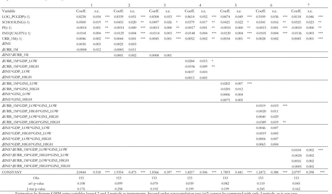
Tables 3 and 4 report results for 7 different specifications (in Table 3 we used URB_1M as measure for agglomeration, while in Table 4 we used URB).26 We started by considering the two variables reflecting
increasing inequality and increasing agglomeration - the variables in changes - (results in column 1). We then further add and interaction term between the two variables (column 2). Specification 3 only introduces the interaction term. To account for nonlinearities, and according to Partridge (1997) and Barro (2000), it is important to distinguish whether the country has a low or high income; specification 4 categorizes each country relative to each period median (GPD_LOW and GDP_HIGH, respectively). According to Chen (2003) the effect of increasing inequality depends on initial levels of inequality; specification 5 distinguishes between initially equal and unequal countries (GINI_LOW and GINI_HIGH, respectively and again using each period median). Specification 6 mixes both criteria; thus, it segregates the effects between four groups of countries depending on a country’s initial conditions (i.e., whether its initial levels of inequality and income are low or high). Specification 7 considers both processes - increasing inequality and increasing agglomeration - interacting with each other and again for the different inequality and income levels. All seven specifications are made by System-GMM using two-step estimation, Windmeijer’s (2005) finite sample robust error correction and limiting the lag depth of the instruments as possible to avoid instrument proliferation.
Our results (Table 3) are consistent with previous literature. Controls have the expected sign and are always significant. Likewise, while inequality is associated with lower growth, urban concentration is associated with higher growth. Furthermore, our results also highlight: 1) growth in agglomeration - measured as the within country’s change in URB_1M - seems to have a significant effect, but it varies with the level of development, as in Brülhart and Sbergami (2009). Thus, there is a positive association in the early stages of development (low income), but becoming negative thereafter (specification 4). However, the significance of the positive association disappears not only when income levels are high, but also when
26 We report ar1 and Hansen tests for validity of instruments in the results tables. Due to the shortness of our panel and the use of
variables in changes, ar2 tests can only be computed as robustness checks from estimations similar than those presented but omitting the variables in changes (in order to gain an extra time period). Key results for the rest of the variables do not change and serial correlation does not appear to be a problem. As for evidence regarding the strength of our instrument set, as Bazzi and Clemens (2013) highlight, there is yet no reliable and straightforward test for Sys-GMM estimations. However, an analysis of correlations for our key variables reveals substantial explanatory power for lagged differences to explain levels and for lagged levels to explain first differences.
inequality levels are high (specification 5). Moreover, it is only when both these levels are low that increasing urban concentration is good for growth. If income and inequality are both high, the coefficient becomes significantly negative (specification 6). 2) In the case of increasing inequality, the coefficient for the change in inequality over time is insignificant in all specifications. However, specification 7 suggests that increasing inequality can be good for growth when combined with increasing agglomeration. This can be interpreted as capital accumulation, but again as long as countries do not already have high levels of income and inequality.
In relation to the policy debate on agglomeration at country level, what these results suggest is that while urban concentration might be associated with economic development, the process of increasing urban concentration (the ten-year increase) might have opposing effects depending on the circumstances of each country; positive effects in developing countries with relatively good income distribution, non-significant in rich countries, and even negative in those with relatively high inequality. Hence, for the OECD context of relatively high-income countries, these findings do not support pro-agglomeration policies. In developing countries, pro-agglomeration policies may be conducive to subsequent growth only when the concentration of resources has not already gone too far (i.e. in low-income-low-inequality countries).
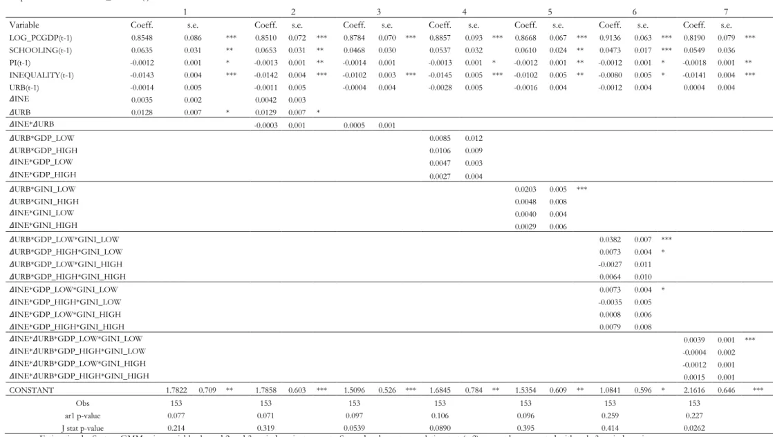
As a simple robustness check to our results, and also to enrich our analysis, we reproduced the estimations using URB, our urbanisation variable, (Table 4) rather than using urban concentration.27 We
obtained slightly different results. Although higher initial levels of urbanisation do not seem to affect growth, the coefficient for increasing urbanisation (i.e. the within country’s change in URB) is positive and significant (specification 1 and 2). As such, increasing urbanisation seems to be good for growth. However, our key result holds; the positive effect from agglomeration is no longer significant when inequality is high (specifications 5, 6 and 7). As for increasing inequality, this variable seems to have a significant and positive effect on growth, but again only in low-income, low-inequality countries (specification 6 and 7).
27 While urban concentration rates only give us information on the role of large agglomerations, more likely to be subject of
congestion diseconomies, urbanisation rates also inform us of the role of small to medium-sized cities. When we experimented with the other measures considered for agglomeration at country level (PRIMACY, GEO_CONC and DENSITY) our key results did not vary much. Here we only present results for URB and URB_1M. These urbanisation measures, besides being the most widely used, capture the agglomeration of population and economic activity and seem to relate more closely to the analysis conducted here, as our results show.
A comparison of the results in Tables 3 and 4 seems to tell us that high urban concentration levels are positively related to subsequent economic growth, while the correlation with urbanisation levels is not significant. However, it might be the case that for small to medium-sized cities (where higher rates of urbanisation do not necessarily imply greater urban concentration at country levels), the process of increasing agglomeration, as opposed to its level, is indeed positively related to growth.28 This occurs, in
particular and again, if inequality levels remain relatively low. A further difference between the results obtained with URB and those obtained with URB_1M is that increasing urbanisation (URB) seems to be positive and significant for the full sample of countries, while increasing urban concentration is positive and significant only for low-income countries, and can even degenerate into congestion diseconomies outweighing the benefits from agglomeration in rich countries.
28 Following recent evidence suggesting that economic growth today is given in small to medium-sized cities, especially in developed
countries (McCann 2012). If we look at the association between economic growth and urbanisation processes decade by decade in our sample, we find that while in the 1980s and 1990s economic growth seems more closely associated with increasing urban concentration, during the 2000s economic growth is far more correlated with increasing urbanisation in small to medium-sized cities - urbanisation that does not take place in agglomeration of more than 1 million inhabitants (Castells-Quintana and Royuela 2014b).
Table 3: Estimations using URB_1M as measure for agglomeration
Dependent Variable: LOG_PCGDP(t)
1 2 3 4 5 6 7
Variable Coeff. s.e. Coeff. s.e. Coeff. s.e. Coeff. s.e. Coeff. s.e. Coeff. s.e. Coeff. s.e.
LOG_PCGDP(t-1) 0.8238 0.054 *** 0.8339 0.051 *** 0.8308 0.053 *** 0.8614 0.052 *** 0.8474 0.049 *** 0.9109 0.036 *** 0.8118 0.046 *** SCHOOLING(t-1) 0.0500 0.019 ** 0.0453 0.020 ** 0.0497 0.026 * 0.0379 0.017 ** 0.0421 0.022 * 0.0341 0.016 ** 0.0525 0.023 ** PI(t-1) -0.0014 0.001 ** -0.0014 0.000 *** -0.0011 0.000 ** -0.0017 0.001 ** -0.0010 0.000 ** -0.0015 0.001 *** -0.0010 0.000 ** INEQUALITY(t-1) -0.0141 0.004 *** -0.0129 0.004 *** -0.0114 0.003 *** -0.0148 0.004 *** -0.0120 0.004 *** -0.0105 0.004 *** -0.0136 0.003 *** URB_1M(t-1) 0.0046 0.002 *** 0.0044 0.001 *** 0.0045 0.001 *** 0.0052 0.002 ** 0.0034 0.001 ** 0.0028 0.002 0.0045 0.001 *** 𝛥INE 0.0030 0.003 0.0025 0.003 𝛥URB_1M -0.0008 0.012 -0.0001 0.011 𝛥INE*𝛥URB_1M 0.0001 0.002 0.0008 0.001 𝛥URB_1M*GDP_LOW 0.0284 0.015 * 𝛥URB_1M*GDP_HIGH -0.0196 0.009 ** 𝛥INE*GDP_LOW 0.0037 0.003 𝛥INE*GDP_HIGH 0.0013 0.005 𝛥URB_1M*GINI_LOW 0.0202 0.007 *** 𝛥URB_1M*GINI_HIGH -0.0201 0.012 𝛥INE*GINI_LOW 0.0006 0.004 𝛥INE*GINI_HIGH 0.0075 0.005 𝛥URB_1M*GDP_LOW*GINI_LOW 0.0519 0.019 *** 𝛥URB_1M*GDP_HIGH*GINI_LOW -0.0020 0.011 𝛥URB_1M*GDP_LOW*GINI_HIGH 0.0040 0.029 𝛥URB_1M*GDP_HIGH*GINI_HIGH -0.0389 0.019 ** 𝛥INE*GDP_LOW*GINI_LOW 0.0046 0.007 𝛥INE*GDP_HIGH*GINI_LOW -0.0019 0.005 𝛥INE*GDP_LOW*GINI_HIGH 0.0004 0.007 𝛥INE*GDP_HIGH*GINI_HIGH 0.0063 0.004 𝛥INE*𝛥URB_1M*GDP_LOW*GINI_LOW 0.0104 0.002 *** 𝛥INE*𝛥URB_1M*GDP_HIGH*GINI_LOW -0.0024 0.002 𝛥INE*𝛥URB_1M*GDP_LOW*GINI_HIGH 0.0016 0.002 𝛥INE*𝛥URB_1M*GDP_HIGH*GINI_HIGH -0.0005 0.002 CONSTANT 2.0444 0.518 *** 1.9354 0.475 *** 1.8366 0.397 *** 1.8217 0.506 *** 1.7893 0.441 *** 1.2472 0.388 *** 2.0797 0.398 *** Obs 153 153 153 153 153 153 153 ar1 p-value 0.108 0.099 0.070 0.039 0.082 0.110 0.045 J stat p-value 0.176 0.258 0.192 0.199 0.199 0.245 0.162
Estimation by System GMM using variables lagged 2 and 3 periods as instruments. Second order autocorrelation test (ar2) cannot be computed with only 3 periods, as is our case.
Table 4: Estimations using URB as measure for agglomeration
Dependent Variable: LOG_PCGDP(t)
1 2 3 4 5 6 7
Variable Coeff. s.e. Coeff. s.e. Coeff. s.e. Coeff. s.e. Coeff. s.e. Coeff. s.e. Coeff. s.e.
LOG_PCGDP(t-1) 0.8548 0.086 *** 0.8510 0.072 *** 0.8784 0.070 *** 0.8857 0.093 *** 0.8668 0.067 *** 0.9136 0.063 *** 0.8190 0.079 *** SCHOOLING(t-1) 0.0635 0.031 ** 0.0653 0.031 ** 0.0468 0.030 0.0537 0.032 0.0610 0.024 ** 0.0473 0.017 *** 0.0549 0.036 PI(t-1) -0.0012 0.001 * -0.0013 0.001 ** -0.0014 0.001 -0.0013 0.001 * -0.0012 0.001 ** -0.0012 0.001 * -0.0018 0.001 ** INEQUALITY(t-1) -0.0143 0.004 *** -0.0142 0.004 *** -0.0102 0.003 *** -0.0145 0.005 *** -0.0102 0.005 ** -0.0080 0.005 * -0.0141 0.004 *** URB(t-1) -0.0014 0.005 -0.0011 0.005 -0.0004 0.004 -0.0028 0.005 -0.0016 0.004 -0.0012 0.004 0.0004 0.004 𝛥INE 0.0035 0.002 0.0042 0.003 𝛥URB 0.0128 0.007 * 0.0129 0.007 * 𝛥INE*𝛥URB -0.0003 0.001 0.0005 0.001 𝛥URB*GDP_LOW 0.0085 0.012 𝛥URB*GDP_HIGH 0.0106 0.009 𝛥INE*GDP_LOW 0.0047 0.003 𝛥INE*GDP_HIGH 0.0027 0.004 𝛥URB*GINI_LOW 0.0203 0.005 *** 𝛥URB*GINI_HIGH 0.0048 0.008 𝛥INE*GINI_LOW 0.0040 0.004 𝛥INE*GINI_HIGH 0.0029 0.006 𝛥URB*GDP_LOW*GINI_LOW 0.0382 0.007 *** 𝛥URB*GDP_HIGH*GINI_LOW 0.0073 0.004 * 𝛥URB*GDP_LOW*GINI_HIGH -0.0027 0.011 𝛥URB*GDP_HIGH*GINI_HIGH 0.0064 0.010 𝛥INE*GDP_LOW*GINI_LOW 0.0073 0.004 * 𝛥INE*GDP_HIGH*GINI_LOW -0.0035 0.005 𝛥INE*GDP_LOW*GINI_HIGH 0.0008 0.006 𝛥INE*GDP_HIGH*GINI_HIGH 0.0079 0.008 𝛥INE*𝛥URB*GDP_LOW*GINI_LOW 0.0039 0.001 *** 𝛥INE*𝛥URB*GDP_HIGH*GINI_LOW -0.0004 0.002 𝛥INE*𝛥URB*GDP_LOW*GINI_HIGH -0.0012 0.001 𝛥INE*𝛥URB*GDP_HIGH*GINI_HIGH 0.0015 0.001 CONSTANT 1.7822 0.709 ** 1.7858 0.603 *** 1.5096 0.526 *** 1.6845 0.784 ** 1.5354 0.609 ** 1.0841 0.596 * 2.1616 0.646 *** Obs 153 153 153 153 153 153 153 ar1 p-value 0.077 0.071 0.097 0.106 0.096 0.259 0.227 J stat p-value 0.214 0.319 0.0539 0.0890 0.395 0.414 0.0262
4. SUMMARY AND CONCLUSIONS
This paper has studied the effects of income inequality and agglomeration at country level on economic growth. In doing so, we have taken into account not only the levels but also the evolution of the variables over time, and the interaction between both processes. Our empirical results seem to show, in line with previous literature, that high inequality levels limit growth in the long run, yet high levels of urban concentration (the proportion of total population living in large cities) seems associated with economic development. Here, the possibilities for higher growth can be associated with the potential growth-enhancing agglomeration economies which countries acquire as economic activity concentrates at the urban level. However, in the case of the processes of increasing inequality and increasing agglomeration (i.e., the variables of change as opposed to those associated with levels), initial conditions seem fundamental, whether the country is relatively poor or rich but also whether income levels are relatively equal or unequal. On the one hand, increasing agglomeration - be it increasing urbanisation or increasing urban concentration - fosters growth in low-income countries; on the other hand, increasing urbanisation, as opposed to increasing urban concentration, seems beneficial for high-income countries. The key outcome is that in both high- and low-income countries, the positive effects of increasing agglomeration are felt in low-inequality countries. When inequality is particularly high, that is not the case, with congestion diseconomies of large cities in high-income countries actually seeming to outweigh the benefits from urban concentration.
The policy implications of these findings vary according to the level of development. In the case of low-income countries, it has been argued that they should pursue growth first and then, when growth is secured, tackle problems of distribution - the frequently argued trade-off between efficiency and equity. This acknowledges the empirical fact that growth is by nature, and at least in the short-run, uneven. This unevenness is, quite crucially, also spatial, associated with the geographical concentration of economic activity (WDR 2009). Yet, it also seems quite clear that sooner or later, inequality becomes a handicap to growth. Indeed, developing countries that face high inequalities also face greater obstacles to achieving sustained long-run economic growth. Both facts taken together mean that while achieving higher economic growth may imply greater inequality due to a greater geographical concentration of economic activity in the short run, it might also mean efforts for better income distribution in the long run as a way of reinforcing,
as opposed to confronting, economic growth. For high-income countries, congestion diseconomies from urban concentration would seem to be a relevant issue that has to be addressed. A more balanced urban system, in which small and medium-sized cities play a fundamental role in the mobilization of local assets to exploit local synergies, seems to be a better strategy than intense urban concentration (OECD 2009). Finally, the fact that the benefits to be derived from agglomeration seem to depend on income distribution appears to point to the relevance of socio-economic and institutional factors in the process of development, particularly in relation to economic geography. Clearly, the subject deserves further analysis and research.
References
Adelman I, Robinson S (1989) Income distribution and development In: Chenery, H and Srinivasan, TN (ed) Handbook of Development Economics, Volume II Elsevier, pp 949-1003
Alesina A, Rodrik D (1994) Distributive politics and economic growth. The Quarterly Journal of Economics 109:465-490
Angotti T (1996) Latin American Urbanization and Planning: Inequality and Unsustainability in North and South. Latin American Perspectives 23(4):12-34
Atkinson A, Brandolini A (2010) On analyzing the World Distribution of Income. The World Bank Economic Review 24(1):1-37
Banerjee A V, Duflo E (2003) Inequality and Growth: What Can the Data Say? Journal of Economic Growth 8(3):267-299
Barca F, McCann P, Rodríguez-Pose A (2012) The case for regional development intervention: Place-based versus place-neutral approaches. Journal of Regional Science 52(1):134-152
Barro R J (1998) Determinants of economic growth: a cross-country empirical study. MIT Press Books The MIT Press, edition 1, volume 1, number 0262522543, December
Barro R J (2000) Inequality and growth in a panel of countries. Journal of Economic Growth 5:5-32
Barro R J (2003) Determinants of Economic Growth in a Panel of Countries. Annals of Economics and Finance 4:231-274
Behrens K, Robert-Nicoud F (2011) Survival of the fittest in cities: Agglomeration, polarization, and inequality, CIRPÉE Discussion Paper #09-19
Bazzi S, Clemens M A (2013) Blunt Instruments: Avoiding Common Pitfalls in Identifying the Causes of Economic Growth. American Economic Journal: Macroeconomics, forthcoming
Bertinelli L, Strobl E (2007) Urbanisation, Urban Concentration and Economic Development. Urban Studies 44(13):2499-2510
Bloom D E, Canning D, Fink G (2008) Urbanization and the wealth of nations. Science 319(5864):772-5
Blundell R, Bond S (1998) Initial Conditions and Moment Restrictions in Dynamic Panel Data Models. Journal of Econometrics 87:115-143
Brülhart M, Mathys NA (2008) Sectoral agglomeration economies in a panel of European regions. Regional Science and Urban Economics 38:348-362
Brülhart M, Sbergami F (2009) Agglomeration and growth: Cross-country evidence. Journal of Urban Economics 65(1):48-63
Camagni R, Capello R, Caragliu A (2013) One or infinite optimal city sizes? In search for and equilibrium size for cities. Annals of Regional Science 51:309-341
Castells-Quintana D, Royuela V (2014a) Tracking positive and negative effects of income inequality on long-run growth. AQR-IREA Working Paper series # 2014/1.
Castells-Quintana D, Royuela V (2014b) Are increasing inequality and urbanization symptoms of growth? Applied Spatial Analysis and Policy (forthcoming)
Chen B (2003) An inverted-U relationship between inequality and long-run growth. Economic Letters 78:205-212 Clarke G (1995) More evidence on income distribution and growth. Journal of Development Economics 47:403-427 Deininger K, Squire L (1996) New Data Set Measuring Income inequality. The World Bank Economic Review
10(3):565-591
Dixit Avinash K, Stiglitz JE (1977) Monopolistic Competition and Optimum Product Diversity. American Economic Review 67(3):297-308
Dimou M (2008) Urbanisation, Agglomeration Effects and Regional Inequality: an introduction. Région et Développement, n° 27
Dupont V (2007) Do geographical agglomeration, growth and equity conflict? Papers in Regional Science 86:193-213 Duranton G, Puga D (2000) Diversity and Specialisation in Cities: why, where and when does it matter? Urban Studies
37:533
Duranton G, Puga D (2004) Micro-Foundations of Urban Agglomeration Economies. In: JV Henderson and J-F Thisse (ed) Handbook of Urban and Regional Economics Vol. 14, Geography and Cities
Durlauf S, Johnson P, Temple J (2005) Growth Econometrics. In: Philippe Aghion and Steven Durlauf (ed) Handbook of Economic Growth, Elsevier, pp 255-677
Easterly W (2007) Inequality does cause underdevelopment: Insights from a new instrument. Journal of Development Economics 84(2):755-776
Ehrhart C (2009) The effects of inequality on growth: a survey of the theoretical and empirical literature, ECINEQ Working Paper Series 2009-107
Fallah B, Partridge M (2007) The elusive inequality-economic growth relationship: are there differences between cities and the countryside? Annals of Regional Science 41:375-400
Galor O (2009) Inequality and Economic Development: The Modern Perspective. Edward Elgar Publishing Ltd Galor O, Moav O (2004) From Physical to Human Capital Accumulation: Inequality and the Process of Development.
Review of Economic Studies 71(4):1001-1026
Gruen C, Klasen S (2008) Growth, inequality, and welfare: comparisons across time and space. Oxford Economic Papers 60:212-236
Harris JR, Todaro MP (1976) Migration, unemployment and development: a two-sector analysis. American Economic Review 60:126-142
Henderson V (2003) The Urbanization Process and Economic Growth: The So-What Question. Journal of Economic Growth 8:47-71
Heston A, Summers R, Bettina A: Penn World Table Version 7.1. Centre for International Comparisons of Production, Income and Prices. University of Pennsylvania (2012)
Jacobs J (1985) Cities and the wealth of nations. Vintage books
Kim S (2008) Spatial Inequality and Economic Development: Theories, Facts and Policies, Working Paper # 16, Commission on Growth and Development
Krugman P (1991) Geography and trade. London MIT Press/Leuven UP, p142
Kuznets S (1955) Economic Growth and Income Inequality. American Economic Review 45:1-28
Lewis WA (1954) Economic Development with Unlimited Supplies of Labour. The Manchester School 22:139-191 McCann P (2012) Cities, Regions and Economic Performance: History, Myths and Realities, Presentation at the 2012
Barcelona Workshop on Regional and Urban Economics Universidad de Barcelona
OECD (2009a) How Regions Grow. Paris Organization for Economic Cooperation and Development
OECD (2009b) Regions Matter: Economic Recovery, Innovation and Sustainable Development. Paris Organization for Economic Cooperation and Development
OECD (2009c) Regions at a Glance. Paris Organization for Economic Cooperation and Development Partridge M (1997) Is inequality harmful for growth? A note. American Economic Review 87(5):1019-1032
Perotti R (1996) Growth, income distribution and democracy: what the data say? Journal of Economic Growth 1:149-187
Persson T, Tabellini G (1994) Is Inequality Harmful for Growth? Theory and evidence. American Economic Review 84:600-21
Rauch JE (1993) Economic Development, Urban underemployment, and Income Inequality. Canadian Journal of Economics 26:901-18
Ross J (2000) Development theory and the economics of growth. The University of Michigan Press
Rosenthal S, Strange W (2004) Evidence on the Nature and Sources of Agglomeration Economies. In: JV Henderson and J-F Thisse (ed) Handbook of Urban and Regional Economics, Vol. 14, Geography and Cities
Robinson J, Acemoglu D, Johnson S (2005) Institutions as a Fundamental Cause of Long-Run Growth. In: Philippe Aghion and Steven Durlauf (ed) Handbook of Economic Growth 1A: 386-472
Robinson S (1976) A Note on the U- Hypothesis Relating Income Inequality and Economic Development. American Economic Review 66(3):437-440
Sala-i-Martin, X, Doppelhofer, G, and Miller, R I (2004) Determinants of long-term growth: A Bayesian averaging of classical estimates (BACE) approach. American Economic Review 3:813–835
Spence M, Clarke P, Buckley RM (Editors) (2009) Urbanization and growth. Commission on Growth and Development, World Bank, Washington
Temple J (1999) The New Growth Evidence. Journal of Economic Literature 37(1):112-156 UN (1993) World Urbanization Prospects: The 1992 Revision. New York: United Nations
United Nations Department of Economic and Social Affairs (2010) World Population Prospects. UN DESA Press UNU-WIDER (1998 onwards) Rising Inequality and Poverty Reduction: Are They Compatible? Research project
Giovanni A Cornia (director) UNU-WIDER
Voitchovsky S (2005) Does the profile of income inequality matter for economic growth? Distinguishing Between the Effects of Inequality in Different Parts of the Income Distribution. Journal of Economic Growth 10(3):273-296 Williamson J (1965) Regional inequality and the process on national development. Economic Development and
Cultural Change 4:3-47
Windmeijer F, (2005) A finite sample correction for the variance of linear efficient two-step GMM estimators. Journal of Econometrics 126(1):25-51
Annex 1: Variables used:
Variable Description Source
GROWTH Cumulative annual average per capita GDP growth rate
Constructed with data from PWT 7.1 (Heston et al. 2012), using real GDP chain data (rgdpch)
LOG_PCGDP Per capita GDP (in log)
Constructed with data from PWT 7.1 (Heston et al. 2012), using real GDP chain data (rgdpch) PI
Price of investment. PPP over investment divided by the
exchange rate times 100 PWT 7.1 (Heston et al. 2012)
SCHOOLING Mean years of schooling, age 15+, total World Bank*
INEQUALITY Gini coefficient Gruen and Klasen 2008**
URB_1M
Population in agglomerations of more than one million as
percentage of total population World Bank
URB Urban population as percentage of total population World Bank
PRIMACY Population in largest city as percentage of urban population World Bank
GEO_CONC Geographical concentration of population Collier 2009
DENSITY Average population by square km of land World Bank
* Missing values for MDG and NGA filled using “IIASA/VID Projection”. ** Missing values filled based on trends: BOL 1980 and 2000, ECU 1980, EGY 1980, HND 1980, KOR 1980, NPL 1990, PER 1980 ZAF 1980, TZA 1980 and ZMB 1990.
Annex 2: List of countries:
Country Country Country
Australia Honduras Norway Bangladesh Hong Kong Pakistan
Belgium Hungary Panama
Bolivia India Peru
Brazil Indonesia Philippines
Canada Ireland Portugal
China Italy South Africa
Colombia Jamaica Spain
Costa Rica Korea, Republic of Sri Lanka Cote d`Ivoire Madagascar Sweden
Denmark Malawi Tanzania
Ecuador Malaysia Thailand
Egypt Mexico Tunisia
El Salvador Morocco Turkey
Finland Nepal United Kingdom
France Netherlands United States
Annex 3: Correlations:
GROWTH LOG_PCGDP INEQUALITY URB URB_1M SCHOOLING PI 𝛥INEQUALITY 𝛥URB
raw data adj. data raw data adj. data raw data adj. data raw data adj. data raw data adj. data raw data adj. data raw data adj.
data raw data adj. data
raw
data adj. data
GROWTH 1.000 1.000 LOG_PCGDP 0.026 -0.588 1.000 1.000 INEQUALITY -0.219 -0.109 -0.443 0.068 1.000 1.000 URB -0.007 -0.085 0.863 0.141 -0.280 -0.135 1.000 1.000 URB_1M 0.063 -0.012 0.486 0.077 -0.146 -0.032 0.625 0.558 1.000 1.000 SCHOOLING 0.170 0.042 0.800 -0.043 -0.312 -0.325 0.741 0.264 0.421 0.228 1.000 1.000 PI -0.165 -0.037 0.143 0.080 -0.101 -0.110 0.235 0.087 0.083 0.070 0.134 -0.052 1.000 1.000 𝛥INEQUALITY 0.026 -0.123 0.004 0.134 0.336 0.748 -0.015 -0.046 0.023 -0.015 0.112 0.046 -0.053 0.006 1.000 1.000 𝛥URB -0.031 -0.068 -0.174 0.158 0.209 0.008 -0.048 0.431 0.054 0.135 -0.223 0.047 -0.170 -0.019 -0.107 0.041 1.000 1.000 𝛥URB_1M 0.001 0.050 -0.131 0.021 0.213 0.046 -0.025 -0.147 0.332 0.091 -0.172 -0.059 -0.090 0.061 -0.029 0.086 0.541 0.365 PRIMACY -0.067 0.200 0.057 -0.161 0.157 0.017 0.078 -0.443 0.492 0.143 0.052 -0.157 -0.043 -0.054 0.003 0.036 0.012 -0.242 GEO_CONC -0.084 -0.083 0.173 0.101 0.107 0.044 0.275 0.199 0.144 0.105 0.142 0.132 0.042 -0.062 0.012 0.068 0.094 -0.152 DENSITY 0.130 -0.078 0.153 0.147 -0.055 0.098 0.241 0.042 0.602 0.320 0.095 -0.095 -0.024 0.068 0.058 0.077 -0.005 -0.055 Adjusted data are obtained by eliminating time and country effects. Observations included: 153 (51 countries x 3 periods). GROWTH, as defined in Annex 1, is measured between t-1 and t. Other variables in levels are measured at t-1. 𝛥 represents change between t-2 and t-1.
Annex 4: Scatter plots among key variables
INEQUALITY vs GROWTH:
URB vs GROWTH:
URB vs INEQUALITY:
Annex 5: Correlations by country´s characteristics:
For low-income-low-inequality countries: 24 observations For high-income-low-inequality countries: 51 observations
GROWTH 𝛥INEQUALITY 𝛥URB 𝛥URB_1M
GROWTH 𝛥INEQUALITY 𝛥URB 𝛥URB_1M
GROWTH 1.000 GROWTH 1.000
𝛥INEQUALITY 0.356 1.000 𝛥INEQUALITY -0.136 1.000
𝛥URB 0.371 0.256 1.000 𝛥URB 0.096 -0.170 1.000
𝛥URB_1M 0.481 0.238 0.701 1.000 𝛥URB_1M 0.130 -0.096 0.401 1.000
For low-income-high-inequality countries: 51 observations For high-income-high-inequality countries: 27 observations
GROWTH 𝛥INEQUALITY 𝛥URB 𝛥URB_1M
GROWTH 𝛥INEQUALITY 𝛥URB 𝛥URB_1M
GROWTH 1.000 GROWTH 1.000
𝛥INEQUALITY 0.129 1.000 𝛥INEQUALITY 0.199 1.000
𝛥URB -0.188 -0.288 1.000 𝛥URB 0.024 -0.552 1.000