New Programming Techniques to Enable and Simplify the Integration of Collaborative Robots in Industrial Environment

(1)

(2)

(3)

Università Politecnica delle Marche

Scuola di Dottorato di Ricerca in Scienze dell’Ingegneria Curriculum in Ingegneria Meccanica

New Programming Techniques to

Enable and Simplify the Integration

of Collaborative Robots in

Industrial Environment

Ph.D. Dissertation of:

Daniele Massa

Advisor:

Prof. Massimo Callegari

Coadvisor:

Ph.D. Cristina Cristalli

Curriculum Supervisor:

Prof. Ferruccio Mandorli

(4)

(5)

Scuola di Dottorato di Ricerca in Scienze dell’Ingegneria Curriculum in Ingegneria Meccanica

New Programming Techniques to

Enable and Simplify the Integration

of Collaborative Robots in

Industrial Environment

Ph.D. Dissertation of:

Daniele Massa

Advisor:

Prof. Massimo Callegari

Coadvisor:

Ph.D. Cristina Cristalli

Curriculum Supervisor:

Prof. Ferruccio Mandorli

(6)

Scuola di Dottorato di Ricerca in Scienze dell’Ingegneria Facoltà di Ingegneria

(7)

Acknowledgments

Thanks to Professor Massimo Callegari and to the group of machine mechanics of DIISM, for supporting me and helping me developing my Ph.D. project in those 3 years. Thanks to the Loccioni Group which gave me the opportunity of taking this academic path, and a special thanks to Cristina Cristalli and my colleagues of Research for Innovation, which supported me in developing and realizing the project. A special thanks also to Arne Roennau and the robotics group of FZI for helping me with the final part of my project. Finally a big thank also to my family that supported me the whole time.

Ancona, Gennaio 2016

(8)

(9)

Abstract

Historically, robots have focused on high volume and highly repetitive tasks, exploiting their precision for those tasks that were boring and/or difficult for humans. But there is a big number of repetitive tasks which is still done by op-erators, which standard industrial robots are not able to do, due to their lack of flexibility and adaptation to new and different contexts. The robot industry is now changing through the introduction of collaborative robots, which are more flexible respect to traditional industrial robots and can work alongside with human operators. This complementarity between industrial robots and collab-orative robots opens many new possibilities both in industrial context and in new fields like service robotics. Moreover, with the coming of Industry 4.0 and Cyber-Physical Systems, the need of having flexible and reconfigurable systems is increasing. To increase the flexibility of industrial robots (collaborative or not) it is needed to develop open source software for robotics programming, to enhance the flexibility and interchangeability of robots. The contribution of this Ph.D. thesis is an analysis of the current state of collaborative robotics, including safety aspects. In addition, this work provides tools that simplify the task of robot programming, making it time-saving and user-friendly, so that no particular knowledge in robotics is required to achieve that. In particular the work is focused on finding sound solutions that can fit the needs of indus-trial contest. Thus, this work proposes innovative methods, validated through experimental results and proposing realistic use-cases, to improve and simplify the robot programming, so to make robots more flexible and well-suited to new needs of Industry 4.0.

(10)

(11)

List of Figures

1.1 Industrial robots market in the last years. . . 1

1.2 Robotics and automation evolution during industrial revolutions. 2 1.3 Cyber-Physical System representation. . . 3

2.1 Safety devices: . . . 9

2.2 Collaborative robots on the market. . . 15

3.1 Overall scheme of the control. . . 20

3.2 Schunk Powerball robotic arm during manual guidance control. The blue, green and red arrows represents respectively x, y and z axis of reference frame. . . 23

3.3 Robot guided through an orientation singularity. Above: Force applied by the human along x, y and z axis (respectively in blue, green and red), the black lines represent the threshold; bottom: The resulting end-effector translational velocity. . . 25

3.4 Robot guided through an orientation singularity. Above: Torque applied by the human around x, y and z axis (respectively in blue, green and red), the black lines represent the threshold; bottom: The resulting end-effector angular velocity. . . 26

3.5 Robot guided through an orientation singularity. Above: trans-lational position of the end-effector along x, y and z axis (re-spectively in blue, green and red); bottom: RPY-orientation of the end-effector. . . 27

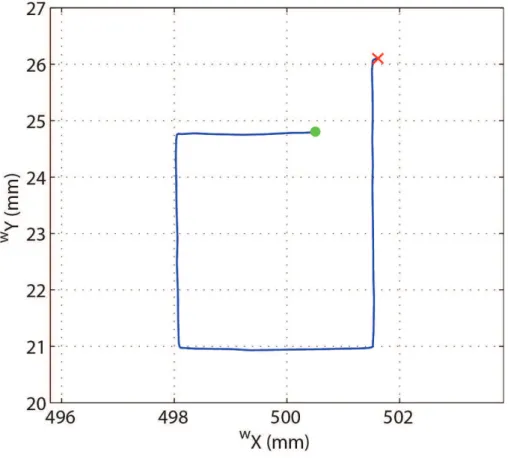
3.6 Robot guided through a rectangle in the x-y plane. Green dot and red cross represents start and end positions respectively. . 28

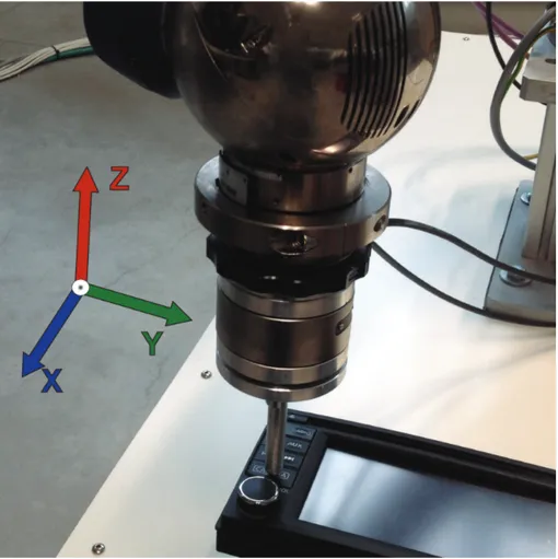
3.7 Schunk Powerball robotic arm testing a front panel. The blue, green and red arrows represents respectively x, y and z axis of reference frame. . . 29

3.8 Teaching to the robot the positions of nine buttons to press. Above: Force applied by the human along x, y and z axis (re-spectively in blue, green and red), the black lines represent the threshold; bottom: The resulting end-effector translational ve-locity. . . 30

(14)

List of Figures

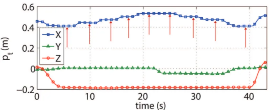
3.9 Teaching to the robot the positions of nine buttons to press. Translational position of the end-effector along x, y and z axis (respectively in blue, green and red); the red arrows show the positions of the nine points that are saved for the reproduction. 30 3.10 Testing a single button. Above: external forces sensed along x,

y, and z axis (respectively in blue, green and red); bottom: total end-effector velocity resulting from equation (3.11). . . 31 4.1 Experimental evaluation of new haptic trajectory exploration for

the force-based PbD approach with a robot arm, force sensor and test work-pieces. . . 34 4.2 Hardware scheme of the work: the robot controller

communi-cates with the URScript programming language with the exter-nal hardware, sending to it the encoders feedback. . . 37 4.3 Characterization of a timing law with trapezoidal velocity profile

in terms of position, velocity and acceleration. . . 38 4.4 Representation and functioning of the used commercial ball

trans-fer unit. . . 40 4.5 Overall work-flow scheme. Under each box is indicated who is

involved in the action; the red arrows represent the work-flow direction, while the yellow arrows point to the phases which are influenced by the force control. . . 41 4.6 Example of task: the operator takes two initial support points,

in this case start (P1) and end point (P2). . . 41 4.7 Example of task: the robot will try to go in straight direction

from the starting point (P1) to the ending point (P2), but it will actually adapt to the surface it finds; the operator can help the robot in this part correcting the tool orientation as desired. . . 42 4.8 Computation of Task Frame. . . 43 4.9 Logic of orientation control: applying a force on the x axis of

the end-effector frame, will produce a movement around the y axis; vice-versa, a force on the y axis will produce a movement around the x axis. . . 44 4.10 Example of task: the robot executes the trajectory learned in

the previous phase; this time the operator can apply forces on the end-effector to modify the path. . . 45 4.11 Task execution example. The table on the right represents an

example of task configuration, while the picture on the left rep-resents the movements the robot will do accordingly to that. . 47 xiv

(15)

List of Figures 4.12 Box task with 4 support points in contact. The superimposed

trajectory is the resulting spline fitting after the first learning phase. . . 48 4.13 Force signal during first learning phase of the box task, along X,

Y and Z axis of task frame, respectively in blue, green and red. The thin dashed lines represent the raw signal obtained from the force sensor, while the thick lines represent the filtered force signal used for the control. . . 48 4.14 3D plots of the second learning phase (left) and reproduction

(right) of the box task, viewed from above. . . 49 4.15 Force signal during second learning phase of the box task, along

X, Y and Z axis of task frame, respectively in blue, green and red. The thin dashed lines represent the raw signal obtained from the force sensor, while the thick lines represent the filtered force signal used for the control. . . 49 4.16 Position error during reproduction of task. The error is

com-puted as the norm of the difference between the expected posi-tion (computed from the spline fitting) and the actual one during reproduction. . . 50 4.17 Force signal during reproduction phase of the box task, along X,

Y and Z axis of task frame, respectively in blue, green and red. The thin dashed lines represent the raw signal obtained from the force sensor, while the thick lines represent the filtered force signal used for the control. . . 50 4.18 Door task with 4 support points. The superimposed trajectory

is the resulting spline fitting after the first learning trajectory. . 51 4.19 Force signal during first learning phase of the box task, along X,

Y and Z axis of task frame, respectively in blue, green and red. The thin dashed lines represent the raw signal obtained from the force sensor, while the thick lines represent the filtered force signal used for the control. . . 52 4.20 3D plots of the second learning phase (left) and reproduction

(right) of the door task, frontal view. . . 52 4.21 Force signal during second learning phase of the door task, along

X, Y and Z axis of task frame, respectively in blue, green and red. The thin dashed lines represent the raw signal obtained from the force sensor, while the thick lines represent the filtered force signal used for the control. . . 53

(16)

List of Figures

4.22 Force signal during reproduction phase of the door task, along X, Y and Z axis of task frame, respectively in blue, green and red. The thin dashed lines represent the raw signal obtained from the force sensor, while the thick lines represent the filtered force signal used for the control. . . 54 5.1 Hardware architecture for open software robotics application. . 55 5.2 Denso industrial robot in manual guidance control. . . 56 5.3 b-CAP protocol slave mode functioning. Above: normal

func-tioning, the interpolation of trajectory is executed inside the RC8 Denso controller. Below: slave mode, the interpolation of trajectory is executed outside the RC8 Denso controller. Source: Denso manual. . . 57 5.4 Hardware configuration for manual guidance experiments with

Denso VS-087 robot. . . 58 5.5 Robot guided through a circle. 3D plot of the end-effector motion. 58 5.6 Robot guided through a circle. Above: Force applied by the

human along x, y and z axis (respectively in blue, green and red), the black lines represent the threshold; bottom: The resulting end-effector translational velocity. . . 59 5.7 Robot guided through a spherical movement. Above: Torque

applied by the human around x, y and z axis (respectively in blue, green and red), the black lines represent the threshold; bottom: The resulting end-effector rotational velocity. . . 60

(17)

Chapter 1 Introduction

In the recent years industrial robotics is having a new spread after the finan-cial crisis of 2009. In 2015 248,000 units were sold worldwide, with a rise of 12 percent respect to the previous year; according to the International Federation of Robotics (IFR) in 2018, about 2.3 millions units will be deployed in fac-tory floors [1]. Nowadays robots used for industrial applications still represents about the 90 percent of the overall robotics market, while service robotics ac-counts for the remaining 10 percent. Speaking of sales, in 2014 the worldwide market value for robots increased to a new peak of 10.7 billions US$, which gets to 32 billions US$ considering the cost of software, peripherals and systems en-gineering. This highlights how the market is fertile both for robot constructors and for system integrators.

Figure 1.1: Industrial robots market in the last years.

The modern robotics industry has its roots with automotive customers. Robots were first used by General Motors in the 1960s and are now

(18)

ubiqui-Chapter 1 Introduction

tous in auto assembly plants globally – penetration of robots in automotive welding for example is now greater than 90 percent. The other big market for industrial robotics is the electrical/electronics industry, which together with the automotive industry constitutes the 65 percent of the overall industrial market for robotics; Figure 1.1 shows the market distribution for industrial robotics in the last years.

Historically, robots have focused on high volume and highly repetitive tasks, exploiting their precision for those tasks that were boring and/or difficult for humans. But there is a big number of repetitive tasks which is still done by operators, which standard industrial robots are not able to do, due to their lack of flexibility and adaptation to new and different contexts. The robot industry is now changing through the introduction of collaborative robots, which are more flexible respect to traditional industrial robots and can work alongside with human operators. This complementarity between industrial robots and collaborative robots, opens a lot of new possibilities both in industrial context and in new fields like service robotics.

Currently collaborative robotics represents just a 5 percent of the overall robotics market, but it is expected to grow tenfold until 2020 (considering both industrial and non-industrial applications), becoming a fundamental actor of the new industrial revolution, Industry 4.0.

Figure 1.2: Robotics and automation evolution during industrial revolutions.

The Industry 4.0 concept has born thanks to the rise of autonomous robots, contemporary automation, cyber-physical systems, the internet of things, the internet of services, and so on.

(19)

Cyber-Physical Systems (CPSs) are the new generation of engineered sys-tems, born from the union of physical devices with networking computing. CPSs are systems featuring a tight combination and integration of computa-tional and physical elements [2]: they are based on computacomputa-tional elements hosted in stand-alone devices, thus extending the concept of embedded sys-tems (see Fig. 1.3). This new kind of syssys-tems is at the base of the Industry 4.0 concept [3] and is expected to bring changes not only in the industrial sphere, but also in the society and our everyday life.

Figure 1.3: Cyber-Physical System representation.

Key features of a CPS are flexibility and adaptability, modularity, autonomy and reliability, safety and efficiency [4]. Cyber-Physical Systems must be able to reconfigure in automatic (or semi-automatic) way and self-organize to change task when needed; in that sense they are modular, meaning that they allow their combination and organization in order to build a more complex system made up by different modules (the single CPS components) communicating between them through the network, exchanging information to accomplish the final overall task. So the spread of CPSs leads to a distributed network of independent but interconnected intelligent autonomous modules, able to com-municate, compute and collaborate. Despite their nature and characteristics make CPSs appear as intrinsically complex systems, they way they interface with humans must be as user-friendly as possible, using mobile devices such as smartphones, tablets and other intuitive equipment [5].

The flexibility and easiness of use of collaborative robots, make them strictly connected to CPS: the objective is to create an intelligent system able to

(20)

per-Chapter 1 Introduction

form dynamic and adaptable movements and to exploit sensor fusion to per-form tasks and collect data, and which is able to collaborate together with other complex systems and with humans.

Until now robot software in the control interface has been mainly proprietary, due to the narrow suite of robot applications – such as material handling and welding - and a relatively concentrated number of suppliers. However, in the last years, the spread of robotics outside of factories and the much wider variety of uses, is leading to the development of open source software for robots control. This means that the software is distributed at source code level and can be re-distributed to others unrestrictedly. The main benefits of this trend are both for developer and for users: open source software leads in fact to collaborative development and to more standardized robotic interfaces, which means both easiness of use, both re-usability of competences and knowledge among different kind of robots. On the other hand open source software would mean a lost of income for providers of proprietary software.

Speaking of academic results, a significant help comes also from the well known software framework ROS (Robot Operating System) [6]. The Robot Operating System is a flexible framework for writing robot software. It is a collection of tools, libraries, and conventions that aim to simplify the task of creating complex and robust robot behavior across a wide variety of robotic platforms and allows to test and reuse works of other researchers in a simple and time-saving way. This also means that algorithms used for one kind of robot can easily be extended and reused for a similar one. As said, this is a need coming directly from the evolution of the new Industry 4.0: ROS is in fact also moving in that direction with ROS-Industrial (ROS-I) [7]. The consortium of ROS-I is made up by both of research institutes and robot constructors and the aim is to extend advanced capabilities of ROS to industrial robots and bring them to manufacturing.

The aim of this Ph.D. thesis is to analyse the current state of collaborative robotics and to provide tools that simplify the task of robot programming, making it time-saving and user-friendly, so that no particular knowledge in robotics is required to achieve that.

Therefore, the second chapter will explain why collaborative robotics is emerging and which are the key functionalities of a collaborative robot, analysing also the safety aspects related to ISO standards. The third chapter will propose a method to implement a manual guidance algorithm using a force/torque sen-sor and will provide experimental results and a use-case. The fourth chapter will focus on those tasks which need the integration of external sensors on the robot, making it difficult to use the basic simplified programming methods that come along with collaborative robots. Thus is here proposed a new method to teach those task in a quick and easy way through few steps. Finally in the fifth 4

(21)

chapter the importance of open source software is highlighted and discussed, and further experimental results are provided.

(22)

(23)

Chapter 2 Collaborative Robotics

The more extensive usage of robots nowadays is still in big companies and enterprises. The needs of small and medium enterprises (SMEs) can be very different and thus it is difficult for them to put money into traditional industrial robots, as the benefits and the income coming from having an industrial robot would not be enough to pay back the initial cost.

Typically SMEs can have a wide range of products which are constantly changing and for each new product the robot would need to be re-programmed accordingly, which is a time-expensive operation. Moreover traditional robotic cells, for safety reasons, must be isolated and closed with physical barriers, which means big amount of space required and low flexibility.

On the other hand, new collaborative robots, i.e. robots intended to phys-ically interact with humans in a shared workspace, have several advantages which can satisfy the needs of SMEs production:

• they are easy to program, which means also spared time for that opera-tion.

• they do not need physical barriers, which means less space is needed. • they are intrinsically safe, thus they can work alongside and with human

operators.

• they can be moved quickly where an increase of production is needed. For those reasons, in the very last years, the usage of collaborative robots is increasing in the SMEs contest, enabling the automation of some repetitive tasks that were still done by humans.

A robot shall be counted as ’Collaborative’ if at least one of the following three conditions is met:

• Manufactured as a ’Collaborative Robot’ - Robot designed for direct in-teraction with a human within a defined collaborative workspace. • Deployed in a ’Collaborative Operation’ - State in which a purposely

(24)

Chapter 2 Collaborative Robotics

• Installed in a ’Collaborative Workspace’ - Space within the operating space where the robot system (including the workpiece) and a human can perform tasks concurrently during production operation.

The traditional and still most diffused method for robot programming is through the robot specific teach pendant. Task trajectories are taught to the robot specifying a set of points which the robot must pass through. However, teaching trajectories to the robot in this way turns out to be very slow and must be done over and over again each time there is a little change in the task. More recently, the availability of more performing hardware and advanced CAE (Computer Aided Engineering) tools promoted the use of off-line programming, which allows to check the feasibility of an industrial operation and even to program a task through the use of a Personal Computer, without the need to stop the production system. In this way the availability of kinematic models of the robot and of the corresponding simulation packages, opens a new range of capabilities, but on the other side an expert Engineer is needed to program the robot.

The necessity of easy programming in industrial context is also urged by the needs of the final customers; industry calls for robotic cells that are more and more flexible, modular and adaptable to different production requirements. The demand for an increasingly high productivity level in industrial manufac-turing scenarios requires both shorter task execution times and faster robotic systems programming cycles. Moreover, the operator often is not a robotics expert, and teach-pendant programming has become a time-consuming and demanding task to be performed.

New collaborative robots on the other hand, can all be programmed in an easy and intuitive way. The operator can in fact take the robot by hand, thanks to different methods of manual guidance, and move it to the desired positions needed for the task, record the positions and subsequently use them for task programming. Moreover some collaborative robots have also some templates that can be used to program simple tasks (i.e. pick and place) even faster.

2.1 Safety in human-robot interaction

This new way of approaching robot programming brings with it a significant problem: the safety in physical human-robot interaction [8], which is a fun-damental aspect of manual guidance. The main standards for granting a safe operation of industrial robots in factories are given by ISO 10218-1/2 [9, 10]; other safety norms, regarding the safe distance to be maintained between hu-man and robots are contained in ISO 13855 [11]. In addition, since the inter-action between humans and robots is now a very relevant argument inside the 8

(25)

2.1 Safety in human-robot interaction robotics community, a new Technical specification (ISO/TS 15066 [12]) about this topic has been recently developed.

(a) Sick Laser Scanner (b) Safety Light Curtains

(c) Pilz SafetyEYE (d) SafetyEYE functioning

Figure 2.1: Safety devices: .

Accordingly to ISO standards, in order to use a non-collaborative industrial robot without physical barriers, some safety sensors can be used to monitor the area around the robot: if someone gets too close to the working area of the robot, then the robot is stopped with a safety stop function. Some safety sensors are showed in Figure 2.1 The computation of the minimum distance between human and robot below which the robot must stop [11], takes into account: the maximum speed of the robot, the theoretical maximum speed of the human, stopping time of the robot and the parameters. This distance could result often in a quite big distance if only horizontal sensors are used (it can easily reach 2 meters), which could mean frequent stops of the robot or big free space around the robot required. A way to reduce this minimum distance is to use both horizontal and vertical safety sensors, in order to create a virtual barrier around the robot, while also monitoring if someone approaches. Finally some robots controllers have the possibility to reduce in a safe way the maximum speed of the robot. In that way, two (or more, depending on the

(26)

controller and on the safety sensors) distances can be computed: the bigger one at which the robot does not stop, but reduces in a safe way its speed; the smaller one at which the robot stops. In that way the distance at which the robot stops is reduced even more.

The new technical specification ISO/TS 15066 specifies 4 different kinds of collaborative operations, which represent the only ways in which is possible to interact with a robot in a safe way:

• Safety-rated monitored stop • Hand guiding

• Speed and separation monitoring • Power and force limiting

The safety-rated monitored stop is the most basic collaborative operation: when the human operator enters the collaborative workspace (which should be monitored with some safety sensor as described above), the robot stops in a safe way. Once the operator exits the collaborative workspace, the robot can resume its work automatically, without the need of additional intervention by the user. Despite being very simple this function permits to share a workspace between human and robot.

Through the hand guiding (or manual guidance) collaborative operation, an operator can use a hand-operated device to transmit motion commands to the robot. The robot must move using a safety-rated monitored speed function to limit the maximum speed of the robot. The hand-operated device must be equipped with a enabling device and an emergency stop, usually mounted on the teach pendant or directly on the end-effector of the robot. This method also permits to integrate the hand guiding operation with some additional features, such as force amplification, virtual safety zones or tracking technologies, in order to improve the manual guidance experience for the operator and/or to prevent the operator from guiding the robot in some areas where he is not supposed to. Ideally, manual guidance methods can be implemented on any industrial robot which is complying with the specification of having a safety-rated monitored speed function and which is having a proper hand-opesafety-rated device.

With the speed and separation monitoring collaborative operation, the robot and the operator may move concurrently in the collaborative workspace. The risk reduction is achieved by maintaining at least the protective separation distance between operator and robot at all times as described as follows:

Sp(t0) = Sh+ Sr+ Ss+ C + Zd+ Zr,

(27)

2.1 Safety in human-robot interaction where Sp(t0) is the protective separation distance at time t0, ShSrand Ssare

the contribution to the separation distance attributable respectively to: the operator’s change in location, the robot reaction time and the robot’s stopping distance. C is the intrusion distance, as defined in ISO 13855, which is the distance that a part of the body can intrude into the sensing field before it is detected. Finally Zd and Zr are the position uncertainties of the operator

and of the robot respectively. The intrusion distance C can be reduced if both horizontal and vertical safety sensors are used, as the body of the operator is detected as soon as it enters the sensing field. During robot motion, the robot never gets closer to the operator than the protective separation distance and when the separation distance decreases to a value below the protective separation distance, the robot system stops with a safety-rated stop function. When the operator moves away from the robot system, the robot can resume motion automatically, while maintaining the protective separation distance. When the robot system reduces its speed, the protective separation distance decreases correspondingly. In that way the robot and the operator can share part of the collaborative workspace, without the need to completely stop the robot motion.

Finally the last collaborative operation, the power and force limiting, is prob-ably the most important one, as describes the specification for robot manufac-turers to build collaborative robots. The ISO/TS 15066 specifies 3 contact situations:

• intended contact situations that are part of the application sequence; • incidental contact situations, which can be a consequence of not following

working procedures, but without a technical failure; • failure modes that lead to contact situations; it also divides the types of contacts into two categories:

• Quasi-static contact: This includes clamping or crushing situations in which a person’s body part is trapped between a moving part of the robot and another fixed or moving part of the work cell. In such a situation, the robot would apply a pressure or force to the trapped body part for an extended time interval until the condition can be alleviated.

• Transient contact (or dynamic impact): This describes a situation in which a person’s body part is impacted by a moving part of the robot and can recoil or retract from the robot without clamping or trapping the contacted body area, thus making for a short duration of the actual contact.

(28)

So, one the main reasons why collaborative robots can work alongside humans without physical barriers and without safety sensors is their capability of sens-ing collisions and properly react to them. There are different ways with which robot can sense collisions: the most precise one (but also the most expensive) is to have joint torque sensors mounted at each joint of the robot. Knowing the planned torque which has been commanded to the robot and making a com-parison with the actual one measured from the sensors, some residual can be computed in order to detect collisions [13]. Clearly such an approach requires the robot to react very quickly when a collision occurs in order to be safe. Fi-nally the ISO/TS 15066 establish also the maximum amount of force/pressure that the robot should not exceed, so that the robot cannot injury the human operators in a severe way. That’s why most of collaborative robots have also a round and ergonomic shape, without edges and sometimes also with some soft covers, in order to reduce the impact force of the robot during unexpected collisions.

However having a collaborative robot, does not necessarily means that it can always be used alongside human operators. In fact if the robot is carrying an end-effector (or handling some components) that can be potentially danger-ous for humans (sharp edges, heavy and rigid components, etc.), the overall solution could not be any more considered safe and collaborative. In order to understand the potential risks of an application, just like for other machines, a risk assessment must be done, in order to prevent and/or limit possible hazards for humans.

2.2 Collaborative robots on the market

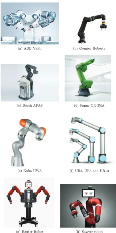
Today, a wide range of collaborative robots (Figure 2.2) which are compliant to ISO safety standards can be found on the market, differing for technical specification (like speed, repeatability, payload), but also for cost.

The ABB YuMi is a collaborative dual-arm robot targeted for electronic assembly market, or in general to handle small and light parts. The two arms have soft components to prevent dangerous collisions; moreover the robot comes with a special wrist mechanism to prevent crush injuries, thanks to which if the robot senses elevated forces applied at the end-effector it puts the last two joints of that arm in a completely passive behaviour and stops the task it was performing. The YuMi is very compact and quite light robot (38 kg, including the controller which is in the "torso"), and the two 7-DOF arms give great flexibility to perform the most challenging manipulation tasks. On the other side the very low payload (0.5 kg per arm; 0.25 kg per arm, if it mounts one of its default grippers, which can include a vacuum cup and a smart camera) limits the possible uses.

(29)

2.2 Collaborative robots on the market Recently, ABB bought another company (Gomtec), which realized the col-laborative robot Roberta. There were three versions of Roberta, differing for payload (4 kg, 8 kg and 12 kg) and for reach(600 mm, 800 mm and 1200 mm). A peculiarity of this robot was the very intuitive programming, which could also memorize and reproduce whole trajectories; all the different modes were selectable rotating a ring on the end-effector, so it was possible to teach a task without using any teach-pendant, but just interacting with the robot. Soon ABB should release a new version of the Roberta robot.

The APAS collaborative solution from Bosch consists of a standard industrial robot with a tactile soft skin to detect unexpected collisions, giving instant feedback to the controller which stops the robot. To use this solution the robot controller must have the safety-rated monitored stop and safety-rated monitored velocity functions. The robotic arm is mounted on a mobile platform that can be moved manually, so to be able to quickly move the robot where needed. Moreover the area around the robot is also monitored and the robot slows down its task when someone gets too close. Finally the APAS robot comes with a 3-finger gripper and with integrated cameras (2D or 3D).

The new green robot from Fanuc (CR-35iA), is the collaborative robot that is closest to traditional industrial robots, speaking of repeatability, reach and payload. The CR-35iA is able to carry weights up to 35 kg with a repeatability of ±0.08mm and has 1813 mm of reach. With this specifications the robot is able to do tasks that other collaborative robots could not be able to do, still being safe thanks to the soft cover and the torque sensors mounted at each joint. On the other hand the robot from Fanuc is less flexible, as it is quite heavy and its pedestal is designed to be fixed to the ground, so it can not be moved easily from one place to another like the other collaborative robots.

The 7-DOF robotic arm Kuka IIWA (Intelligent Industrial Work Assistant) is the evolution of the LWR 4+ in terms of physical features: the robot is in fact equipped with torque sensors on each joint, has high-performance collision detection algorithms and has an incredibly good ratio between weight and payload. The controller (the Kuka Sunrise) is instead quite different from the previous version, as it uses Java as programming language, offering a library containing a lot of high-level functions.

The Baxter robot from Rethink Robotics is a very versatile and easy to use robot. In fact in order to use the Baxter robot no programming knowledge is needed and can be trained in few minutes. Moreover Baxter is a complete system, comprehensive of different sensors, so for simple tasks no integration with other hardware is needed. Finally it has a very low price (the starting price is around 20 k$), considering the number of DOFs that the Baxter has and the various sensors and end-effector that can be mounted on it. On the other hand the Baxter robot has a very low precision and repeatability (due to

(30)

mechanical elasticity of joints), which clearly limits the range of applications in which it can be applied.

Sawyer is the more recent collaborative robot from Rethink Robotics. Unlike Baxter, it is made to work in fixed position and it is not mounted on a mobile base. Moreover it is more repeatable respect to the Baxter robot, but still quite far from other collaborative robots. Finally Sawyer mounts a Cognex camera for a more precise vision system and has also force sensing embedded at each joint.

Finally, the robots from Universal Robot consist of six-axis arms of different dimensions: the UR10 can carry up to 10 kg and has a reach of 1600 mm, the UR5 has a 5 kg payload and a reach of 900 mm; finally the newest UR3 has a payload of 3 kg and a reach of 500 mm. All UR robots are quite precise and lightweight, but also quite cheap. As all collaborative robots, they can be moved by hand for a fast teaching. The Universal Robots are probably the collaborative robots that are currently most diffused, especially in industrial context, thanks to their good price (the most expensive one, the UR10 is below 30ke) and their good capabilities.

(31)

2.2 Collaborative robots on the market

(a) ABB YuMi (b) Gomtec Roberta

(c) Bosch APAS (d) Fanuc CR-35iA

(e) Kuka IIWA (f) UR3, UR5 and UR10

(g) Baxter Robot (h) Sawyer robot

(32)

(33)

Chapter 3 Enabling Programming by

Demonstration

The new promising way for robot programming is the Programming by Demon-stration (PbD) [14, 15], which allows the operator to teach to the robot a generalized version of a task in an easy and natural way, thus requiring no experience in robot programming. In the teaching process, apart from the joints position, several measurements can be taken into account and integrated together, such as force profiles or voice commands [16]. These methods can then be customized, depending on the task, in order to handle exceptions us-ing different strategies [17]. An ideal solution would be a scenario where the operator’s movements are tracked while he is doing the task and then, using machine learning methods, the capability of reproducing the task is taught to the robot. This is a challenging topic of research of recent years; in addition, from an industrial point of view these methods are still not robust enough. Moreover, if during the task execution lifting heavy weights is required, the operator could not have enough physical strength to perform the task. As a consequence of this, a method that is more robust and that could manage tasks with heavy weights lifting is the manual guidance (or walk-through). This type of control lets the user move physically the robot by hand in a free way, instead of moving it using the teach pendant; these movements can then be encoded and used for learning a generalized version of the task or for reproduction.

Another way to teach a task to a robot is using haptic devices, which can be used to command velocities to the robot, while giving a force feedback to the user; in this way also force tasks can be taught to the robot. Such devices are very expensive and for this reason at the moment they cannot be adopted in industrial contexts; on the other hand, they are mostly used in medical or rehabilitation robotic applications.

(34)

Chapter 3 Enabling Programming by Demonstration

3.1 Manual Guidance State of Art

In order to achieve robot manual guidance, several control approaches that use different kinds of sensors, or more in general hardware, can be implemented. Most types of control schemes make use of a force/torque sensor mounted at the wrist of the robot; the use of such sensors allows the design of control schemes that grant a very precise motion of the end-effector, such as admit-tance/impedance control [18–20] or force control [21]. The main drawback of the majority of these methods is that, apart from the cost of the force/torque sensor, they rely on the availability of a robust dynamic model of the robotic arm. Other researchers propose advanced variants of both types of control, such as variable impedance control [22], adaptive admittance control [23] or admittance control based on virtual fixtures [24]: these are software-generated motion guidance, based on a vision system that extrapolates the geometry of the robot and of the workspace needed to compute the motion constraints. The hybrid force/motion control, that can be achieved both at kinematic [25] and dynamic level [21], describes the task constraints combining a force control and a velocity control, through selection matrices. Since few years, some new lightweight robots come with an implementation of compliance control, as for example the Kuka LWR IV [26] or its evolution, the Kuka iiwa. Again, this is a clear sign that the whole robotic community is moving towards the robot co-worker concept.

In order to make the operator feel like he/she is moving a tool of reduced mass (instead of an heavy and stiff robot), the dynamics of the robot motion can be described as a “virtual tool”: the end-effector is modelled as a virtual point of chosen mass which can be placed arbitrarily in a free space environment. Then the robot can be controlled using admittance control [27] or a simple kinematic control [28]. Another interesting approach is to mix up the feedback from the force/torque sensor with visual information [29]. Here the maximum end-effector velocity allowed is proportional to the distance between the robot and surrounding obstacles; in that way the robot prevents collisions. Other works have developed a force control without using force sensors, by using observation methods [30] or seeing the external force as a disturbance [31].

Another way to achieve manual guidance is using fault detection and iden-tification (FDI) methods to sense external forces [13]: in this case, external forces can be detected defining a residual that observes and measures differ-ences between the commanded torque and the actual torque. This method has the drawback that the operator must move the joints one by one, thus resulting in an unnatural feeling of motion; moreover the dynamic model of the robot must be available; in the end, this approach is mainly suited for unexpected collisions detection and reaction.

(35)

3.2 Manual Guidance implementation Other works try to use the currents of motors to estimate the torque at each joint [32]: the torque estimation can then be used to achieve manual guidance. In particular, in [33] low-pass and high-pass filters are applied to motors cur-rents to detect human intentional interaction. Despite the innovation of these methods, they are not suited for industrial use, both in terms of robustness and precision of movements. Moreover, the friction of the motor reductor af-fects the readings of the currents, and its effect can change during time and in different temperature conditions [34].

Finally, a more recent way to perform kinesthetic movements is through back-drivability, like the Barret WAM [35], which allows robots with backdrivable motors to be guided by the user keeping them in zero-gravity control mode; these robots are used especially to test learning algorithms [15]. The draw-back of draw-backdrivability is that it is suited only for lightweight or small robots, because of the robot inertia; thus it can not be applied to industrial robots. Moreover, in this case the user must move the joints one by one, which makes it difficult (especially for robots with many degrees of freedom) to perform natural and smooth movements.

3.2 Manual Guidance implementation

In this section, an implementation of manual guidance based on the use of a force/torque sensor is presented. The sensor is mounted between the wrist and the end-effector of the robot, so a gravity compensation of the weight of the tool is needed. in the following subsections the gravity compensation and control algorithms will be explained.

3.2.1 Gravity compensation

In order to distinguish the input force of the user from the gravity force on the end-effector, a static model of the robotic system (i.e. the robotic arm, the force/torque sensor and the end-effector) must be developed. Since the manual guidance application is here considered as semi-static (accelerations applied by the operator are considered to be very small), a full dynamic model is not necessary. Starting from the forces and torques measured by the sensor, respectivelys fmandsτm we have: s fm = s fh+ s g (3.1) s τm = sτh+sτg, (3.2) wheres_f

handsτhare respectively the force and torque applied by the human

operator to the end-effector in sensor frame, whiles_g _ands_τ

(36)

Figure 3.1: Overall scheme of the control.

force and torque acting at the center of mass of the end-effector expressed in sensor frame. Expressing these equations into world frame leads to:

w Rssfm = w fh+ w g (3.3) w Rssτm = wτh+wτg, (3.4) where now w_f

h, wτh, wg and wτg are expressed in world frame; wRs is

the rotation matrix from sensor frame to world frame, computed as w_R s = w_R

eeeeRs, wherewReeis obtained from direct kinematics andeeRsrepresents

the rotation matrix from the sensor frame to end-effector frame (which is con-stant). Equations (3.3-3.4) can be resolved to find out the force/torque applied by human: w fh = w Rssfm− w g (3.5) w τh = wRssτm−wr×wg, (3.6) with w τg= −wr×wg,

where w_g _{is the weight of the end-effector in world frame,} w_r _{is the position}

vector of the center of mass of the end-effector with reference to the origin of the sensor frame, expressed in world frame. In such a way the gravity-compensated force and torque applied by human can be considered in the control loop. For simplicity, in the next subsectionw

fhandwτhwill be referred to as f and τ .

3.2.2 Virtual Tool Controller

The gravity compensated forces and torques, obtained as described in the pre-vious subsection, are fed to a virtual tool controller: it has been reckoned that in comparison with a proportional controller, it would yield a more natural feel-ing for the operator when movfeel-ing the end-effector. The virtual tool controller 20

(37)

3.2 Manual Guidance implementation basically commands an acceleration to the robot end-effector that is propor-tional to the force/torque applied by the human and adds a damping factor to decelerate the robot and make it stop fast when the external force is not applied any more. In this way, the dynamics of the end-effector is modelled as a virtual point whose lumped mass is located at the center of mass of the end-effector. Since the gravity of the real mass of the robot end-effector has been compensated as described in the above subsection, it has not been considered in the controller.

Since the robot is controlled in the velocity domain, the desired translation and rotation end-effector velocities at time t are defined as:

vt t= I (K1(f ± tf) − K2vt_t−1)∆t + vt_t−1, if|f | > tf −K3vt_t−1∆t + vt_t−1, if|f | < tf (3.7) vr t = I (K1(τ ± t_τ) − K2vr_t−1)∆t + vr_t−1, if|τ | > t_τ −K3vr_t−1∆t + vr_t−1, if|τ | < t_τ (3.8)

Equations (3.7) and (3.8) represent the implementation of the virtual tool controller: tf and tτ are threshold vectors for noise filtering, K1, K2 and

K3 are positive diagonal gain matrices and ∆t is the control loop cycle time.

Signs in equations (3.7) and (3.8) depend on the sign of f and τ respectively. Analysing the virtual tool controller, it can be noticed that there is a first term which is proportional to the force and torque applied by the human, and a damping factor which is needed to provide resistance. In particular, when the absolute value of force/torque is smaller than the threshold, the damping factor is needed to decelerate the motion of the robot. This is why two different gain matrices (K2and K3) are used for the two cases: because when no forces are

sensed, the robot needs to decelerate faster. For this reason the elements of

K3 are chosen much bigger than the ones of K2.

Finally the end-effector velocities are transformed in joint velocities:

˙q = J†v, (3.9)

where ˙q is the vector of joint velocities, J†is the pseudo-inverse of the Jacobian (concerning both position and rotation) and v = [vt_vr_]′_{. It is noted that when}

the Jacobian is square and non-singular (i.e. the number of joints is equal to the number of degrees of freedom of the task), a simple inversion of the Jacobian could be used instead.

(38)

ap-Chapter 3 Enabling Programming by Demonstration

proach: forces and torques measured from the sensor are first gravity compen-sated as described in previous section, then used by the virtual tool controller to obtain a velocity reference for the end-effector. This reference is finally mapped on robot’s joints using the pseudo-inverse of the Jacobian.

If the end-effector gets in contact with the environment, the sensor will sense a normal force and will promptly move away from the touch point: such motion will be just a transient effect, characterized by a velocity proportional to the approaching speed and thus to the force sensed by the sensor. If it is needed to interact with the environment (e.g. to follow a profile which has to be deburred) one could manually disable the command along that direction (i.e. probably the end-effector normal axis). However, in the chosen application domain, that is quality control, it is uncommon to need such solution; most of the tasks which need interaction with the environment, can be programmed offline and then the robot must only know “where” to execute the task (e.g. the proposed approach in section 3.4).

Even though robot kinematic singularities are easily avoidable by the user, a solution consists in using a damped pseudo-inverse of the Jacobian, defined as: J†λ= J T1 J JT + λ2 I2 −1 , (3.10)

with damping factor λ << 1; using the SVD decomposition J = U ΣVT_,

equation (3.10) leads to:

J†_λ= V Σ†λU T_,

where Σ†λ is a diagonal matrix, with elements:

˜ σi= σi σ2 i +λ 2,

where σi is the ith singular value of the Jacobian matrix. This means that

J†_λ has singular values ˜σi, with ˜σi → 1/σi for λ → 0. In this way the robot

can pass through singularities, even though obviously only velocities in the manipulability ellipsoid can be accomplished.

3.3 Experimental results

Experiments have been carried out using the Schunk Powerball robotic arm. As Figure 3.2 shows, the Schunk Powerball consists of three modules, each one containing two motors, for a total of six joints. The robotic arm is con-trolled with a personal computer in the velocity domain using the ROS packages

schunk_lwa4p and ipa_canopen. No ROS tools for kinematics or planning

are used, joint velocities are commanded to the robot each 10 milliseconds and 22

(39)

3.3 Experimental results

Figure 3.2: Schunk Powerball robotic arm during manual guidance control. The blue, green and red arrows represents respectively x, y and z axis of reference frame.

these commands are then executed by the internal controller of each module; thus the proposed approach is applicable to any industrial robot, provided that the power needed to control the robot complies with the maximum allowed by ISO standards, which is the case of the Powerball robot. Thus, in order to make the experimental set-up fully compatible with ISO standards, an emer-gency stop and an enabling device to start guiding the robot should be added near the end-effector. The force/torque sensor (KMS40 from Weiss Robotics) is mounted between the sixth joint and the end-effector and communicates with the pc using an ethernet protocol, updating the force and torque signals at a frequency of 500 Hz. So in that case the bottleneck for the algorithm implementation is the robot control frequency (100 Hz), which is the actual frequency at which the algorithm will run. Of course, having an higher control

(40)

frequency would make the control algorithm more reactive to external inputs; anyhow for a manual guidance algorithm, were the inputs come from a human operator (usually at low frequencies), a control loop of 100 Hz brings satisfying results.

The experiments made using the proposed approach resulted in smooth and natural motions of the robot.

Parameters of (3.7) and (3.8) were chosen as follows:

K1=    0.05 0 0 0 0.05 0 0 0 0.05   K2=    2 0 0 0 2 0 0 0 2    K3=    8 0 0 0 8 0 0 0 8   ,

for both the force and torque equations. For the thresholds, the values chosen are the following:

tf =    2 2 2   tτ =    0.65 0.65 0.65   ,

meaning that all forces below 2N and all torques below 0.65N m are considered as noise. All those parameters where chosen experimentally.

The small value of K2 gain makes the robot lighter to the user, while the

high value of K3makes the robot stop almost instantly when no external forces

are sensed. This resulted in a both smooth and precise motion of the robot, achieving the expected result. Experimental results are shown in the remainder of the section.

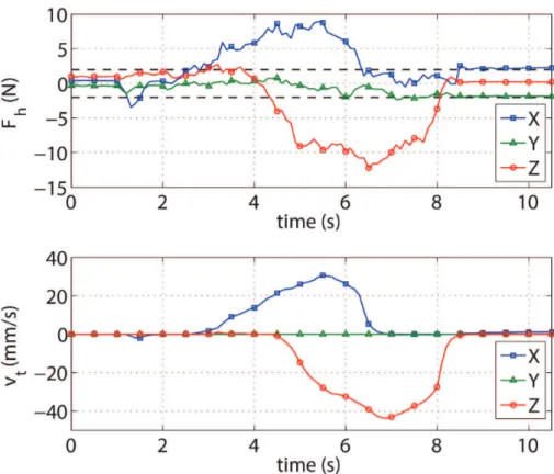
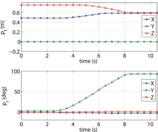
In the first test the robot is moved through an orientation singularity; in particular the 4th _{and 6}th _{joints are aligned. As showed in the plots of}

Fig-ure 3.5, the transition through the singularity results in a smooth movement. Notice that, as Figures 3.3 and 3.4 show, the resulting end-effector velocity is a low-pass filtered version of the force and torque signals; this is fundamental, because a simple proportional controller would be otherwise affected by the noise of the sensor.

The second experiment is carried out to test the precision of movements. In order to make the robot more precise (but also stiffer) the elements of matrix

K1are lowered. The plots in Figure 3.6 show how the operator is able to move

around the robot in a precise way, being able to describe a small rectangle in the x-y plane, while keeping constant the orientation and the position along the z axis. This means that the maximum precision that is achievable is the operator’s precision. Actually the precision could be increased even more, rising 24

(41)

3.4 Use-Case

Figure 3.3: Robot guided through an orientation singularity. Above: Force applied by the human along x, y and z axis (respectively in blue, green and red), the black lines represent the threshold; bottom: The resulting end-effector translational velocity.

the threshold values in equations (3.7) and (3.8); in this way the operator should use more force to move a little the robot and the precision would be the robot’s one. On the other hand this would result in an unnatural feeling for the operator and in a very stiff motion, so should be used only when strictly necessary.

3.4 Use-Case

The implementation of the robot manual guidance described in the above sec-tions can be used to teach a task to the robot. The chosen application domain is the quality control of front panels of electronic devices (Figure 3.7). A useful task that can be taught to the robot is the test of buttons on panels in order to check how much force is needed to press the buttons. The test of panels is a simple task, but due to the continuous changing of the models it is difficult to

(42)

Figure 3.4: Robot guided through an orientation singularity. Above: Torque applied by the human around x, y and z axis (respectively in blue, green and red), the black lines represent the threshold; bottom: The resulting end-effector angular velocity.

automatize; with the proposed approach, each time a new kind of panel must be tested, teaching the new task to the robot can be done in an easy and time-saving way. The user can teach the positions of the buttons by simply bringing the robot’s end-effector above them (so without pressing them) and saving the joint configurations through the user interface. The end-effector of the robot has been designed on purpose: it has the double advantage of making the man-ual guidance algorithm ergonomic and of being able to press buttons for that specific application. In the reproduction of the task, the robot will first move through the saved positions using a simple kinematic control for positioning; when the robot reaches the saved positions, it will then go down along the Z axis direction using an impedance control, implemented as follows:

v= vh+ vI, (3.11)

(43)

3.4 Use-Case

Figure 3.5: Robot guided through an orientation singularity. Above: transla-tional position of the end-effector along x, y and z axis (respec-tively in blue, green and red); bottom: RPY-orientation of the end-effector.

where vhis exactly the velocity obtained from equations (3.7) and (3.8), using a

K1with very low coefficients; the vI is a velocity resulting from the impedance

control, computed as:

vI = Kimp(pr− pEE) , (3.12)

where Kimp is a positive diagonal matrix representing the spring stiffness,

while pr and pEE are respectively the rest position of the virtual spring and

the actual position of the end-effector of the robot; a damping factor is not considered in equation (3.12), since the vh already includes one. Notice that,

in order to make the robot move along the z axis, the point pr is moving.

Moreover, since the robot is desired to be compliant along z-axis and rigid along all other directions, equation (3.11) in practice is only implemented for the z-axis component, while the other components are equal to zero. After the force sensed along the z axis exceeds a maximum value admitted (in this case

(44)

Figure 3.6: Robot guided through a rectangle in the x-y plane. Green dot and red cross represents start and end positions respectively.

15N ), the impedance control is stopped (v = vh), so that the pushing force

does not increase too much. After the robot has pressed a button, it will first go back to the current approach position and then it will move to the next approach position ready to test the next button.

Figures 3.8 and 3.9 respectively show the forces (and the resulting velocities) along the 3 cartesian axis, and the position of the end-effector of the robot during the teaching process of a task. In this task 9 positions (taken above 9 buttons to test) are taught, showed by the red arrows in Figure 3.9; the operator is communicating to the program user interface (pressing a button on a keyboard) that the current position must be saved for reproduction, that is why in these instants the position of the end-effector keeps constant. Again, it can be noticed how the proposed approach results in a smooth and precise movement of the end-effector.

Regarding the reproduction, to make better understand what happens when the robot presses a button, in the plots it is only reported the first of the nine 28

(45)

3.4 Use-Case

Figure 3.7: Schunk Powerball robotic arm testing a front panel. The blue, green and red arrows represents respectively x, y and z axis of reference frame.

taught positions in Figures 3.8 and 3.9. During the reproduction phase the robot first moves with kinematic control to a taught position, and then (Figure 3.10) it will start moving along the negative direction of Z axis in impedance control; the performed experiments show that at the instant when the button is pressed, a small peak of the external force is sensed (see Figure 3.10). In this way the value of the force needed to press the button can be easily found out. It is noted that in the bottom plot of Figure 3.10 the resulting end-effector velocity is only made up of the impedance control effort until the force sensed exceeds the black threshold (top plot of Figure 3.10).

(46)

Figure 3.8: Teaching to the robot the positions of nine buttons to press. Above: Force applied by the human along x, y and z axis (respectively in blue, green and red), the black lines represent the threshold; bottom: The resulting end-effector translational velocity.

Figure 3.9: Teaching to the robot the positions of nine buttons to press. Trans-lational position of the end-effector along x, y and z axis (respec-tively in blue, green and red); the red arrows show the positions of the nine points that are saved for the reproduction.

(47)

3.4 Use-Case

Figure 3.10: Testing a single button. Above: external forces sensed along x, y, and z axis (respectively in blue, green and red); bottom: total end-effector velocity resulting from equation (3.11).

(48)

(49)

Chapter 4 Simplifying Robot Programming

Through Haptic Learning

Without robots, many products of today would not be possible, as their preci-sion, speed and ability to repeat tasks without deviation is an absolutely essen-tial feature for today’s production lines. While iniessen-tially only large companies could afford expensive robots to scale up mass production of goods, they are finally becoming affordable even for small and medium sized businesses. But there is still a major problem with the use of robots in SMEs: Programming robots is very hard, time consuming and expensive [36]

To fulfill the hard requirements of SMEs modern production robots need to be able to work together with the human workers, and adapt quickly to new and complex tasks. Most importantly, the time needed to program these new tasks and the expertise required, needs to be significantly reduced to enable cost effective usage of these complicated tools, as currently the costs for the software outweighs those of the hardware.

As discussed in Chapter 2, new collaborative robots are easier to use and the teaching time is less time-expensive. But what if the task to be taught needs the integration of one or more sensors external to the robot? For example it could be needed a vision system that identifies the work-piece, or the integration of a force sensor for a task where the robot must apply some specified forces. Depending on the task, the easy teaching methods that come out of the box with collaborative robots could not be enough.

One approach to achieve easy robot programming is Programming by Demon-stration (PbD) as previously discussed in chapter 3. Robots are programmed by letting the user demonstrate the task to the robot rather than programming it explicitly, therefore reducing the required robotics knowledge significantly, especially for inexperienced users. After observing the user, the robot adapts the observed movements to its own constraints (like number of joints) and re-produces them. This allows not only to skip calibration and knowledge issues but also allows the robot to learn from user experience which can be very important in the productions of specialized goods where small differences in

(50)

Chapter 4 Simplifying Robot Programming Through Haptic Learning

handling will result in a superior product. But to create a good application and actually harness the power of this approach, the PbD process needs to be well designed, easy to use and most importantly has to reproduce the intended task as accurately as possible. While the idea behind PbD is simple, many

Figure 4.1: Experimental evaluation of new haptic trajectory exploration for the force-based PbD approach with a robot arm, force sensor and test work-pieces.

implementations currently available often lack important features that enable a wide range use or are still time consuming when teaching non trivial tasks. To be successful in real world applications there are some key challenges that a robotic system needs to address:

• Self-adaptation of trajectories: As it is difficult to teach a perfect trajec-tory, the robot should assist the user by adapting to imperfections and work-piece structure.

• Surface Exploration of trajectory: It should be sufficient to just show the basic task and let the robot explore unknown objects and how to execute the trajectory by itself.

• Online user modification: It must be possible to adapt the work-flow easily and change a robot program in an intuitive way and without the need to re-teach everything.

(51)

• Force-based tasks: Facilitating a force control on a standard robot arm increases the number of possible tasks, making the robot more flexible and valuable.

• Intuitive shared programming: Programming a robot needs to combine the benefits of human skill and robotic precision in the most intuitive way to be successful.

Therefore it is here proposed a new approach for haptic trajectory exploration for force-based programming by demonstration consisting of a three step teach in process:

• Demonstration of the desired trajectory is done in an easy and fast way. By teaching a few initial support points above the object, the overall path is defined.

• Haptic trajectory exploration: the robot quickly explores the surface of the object in an automated way, without the need to manually teach additional support points.

• Shared adaptation: creates an executable trajectory along the path for the robot, which the user can easily refine to fit the needs of the applications and assist with very complex parts.

This novel force-based approach is implemented using an off the shelve low cost, light weight robot arm with an attached force sensor, making it transfer-able to almost any robot arm that offers a low level control interface (see Fig. 4.1). Enabling force-based execution and haptic exploration not only provides a much easier teaching experience that can be used with almost no training but also allows to perform complex robot tasks that are impossible with classical teach-pendant programming. The proposed system can be easily added to new or existing set-ups and could greatly lower the time and therefore costs it takes to use robots in difficult tasks.

As explained in Chapter 2, the most obvious and common way of teaching something to a robot is using its dedicated teach-pendant; this allows the op-erator to teach either segments of a path or support points which are to be followed. This method is less complex than programming but still requires some expertise of the operator making it a specialist job that is very time con-suming. Complex paths that follow surfaces closely need a very high number of support points and can take several hours to days to produce good results. Generating the paths from CAD models [37] is a very good way to produce ac-curate paths, even along complex surfaces. Exporting from CAD programs and using it on robots however, is far from a standard procedure. But, even if it is possible, it will usually require fine tuning and calibration by an expert, as the